


Abstract
High-dimensional categorical data are routinely collected in biomedical and social sciences. It is of great importance to build interpretable parsimonious models that perform dimension reduction and uncover meaningful latent structures from such discrete data. Identifiability is a fundamental requirement for valid modeling and inference in such scenarios, yet is challenging to address when there are complex latent structures. In this article, we propose a class of identifiable multilayer (potentially deep) discrete latent structure models for discrete data, termed Bayesian Pyramids. We establish the identifiability of Bayesian Pyramids by developing novel transparent conditions on the pyramid-shaped deep latent directed graph. The proposed identifiability conditions can ensure Bayesian posterior consistency under suitable priors. As an illustration, we consider the two-latent-layer model and propose a Bayesian shrinkage estimation approach. Simulation results for this model corroborate the identifiability and estimatability of model parameters. Applications of the methodology to DNA nucleotide sequence data uncover useful discrete latent features that are highly predictive of sequence types. The proposed framework provides a recipe for interpretable unsupervised learning of discrete data and can be a useful alternative to popular machine learning methods.
1 Introduction
High-dimensional unordered categorical data are ubiquitous in many scientific disciplines, including the DNA nucleotides of A, G, C, T in genetics (Nguyen et al., 2016; Pokholok et al., 2005), occurrences of various species in ecological studies of biodiversity (Ovaskainen & Abrego, 2020; Ovaskainen et al., 2016), responses from psychological and educational assessments or social science surveys (Eysenck et al., 2020; Skinner, 2019), and document data gathered from huge text corpora or publications (Blei et al., 2003; Erosheva et al., 2004). Modeling and extracting information from multivariate discrete data require different statistical methods and theoretical understanding from those for continuous data. In an unsupervised setting, it is an important task to uncover reliable and meaningful latent patterns from the potentially high-dimensional and heterogeneous discrete observations. Ideally, the inferred lower-dimensional latent representations should not only provide scientific insights on their own, but also aid downstream statistical analyses through effective dimension reduction.
Recently, there has been a surge of interest in interpretable machine learning, see Doshi-Velez and Kim (2017), Rudin (2019), and Murdoch et al. (2019), among others. Latent variable approaches, however, have received limited attention in this emerging literature, likely due to the associated complexities. Indeed, deep learning models with many layers of latent variables are usually considered as uninterpretable black boxes. For example, the deep belief network (Hinton et al., 2006; Lee et al., 2009) is a very popular deep learning architecture, but it is generally not reliable to interpret the inferred latent structure. However, for high-dimensional data, it is highly desirable to perform dimension reduction to extract the key signals in the form of lower-dimensional latent representations. If the latent representations are themselves reliable, then they can be viewed as surrogate features of the data and then passed along to existing interpretable machine learning methods for downstream tasks. A key to success in such modeling and analysis processes is the interpretability of the latent structure. This in turn relies crucially on the identifiability of the statistical latent variable model being used.
In statistical terms, a set of parameters for a family of statistical models are said to be identifiable if distinct values of the parameters correspond to distinct distributions of the observed data. Studies under such an identifiability notion date back to Koopmans and Reiersol (1950), Teicher (1961), and Goodman (1974). Model identifiability is a fundamental prerequisite for valid statistical estimation and inference. In the latent variable context, if one wishes to interpret the parameters and latent representations learned using a latent variable model, then identifiability is necessary for making such interpretation meaningful and reproducible. Early considerations of identifiability in the latent variable context can be traced to the seminal work of Anderson and Rubin (1956) for traditional factor analysis. For modern latent variable models potentially containing nonlinear, non-continuous, and even deep layers of latent variables, identifiability issues can be challenging to address.
Recent developments on the identifiability of continuous latent variable models include Drton et al. (2011), Anandkumar et al. (2013), and Chen, Li, et al. (2020). Discrete latent variable models are an appealing alternative to their continuous counterparts in terms of the combination of interpretability and flexibility. Finite mixture models (McLachlan & Basford, 1988) routinely used for model-based clustering are a canonical example involving a single discrete latent variable. Such relatively simple approaches are insufficiently flexible for complex data sets. Extensions with multiple latent variables and/or multilayer structure have distinct advantages in such settings but come with increasingly complex identifiability issues. In this work, we are motivated to build identifiable deep latent variable models, which are flexible enough to capture the complex dependencies in real-world data, yet also with appropriate restrictions and parsimony to yield identifiability.
We propose a family of multilayer, potentially deep, discrete latent variable models and propose novel identifiability conditions for them. We establish identifiability for hierarchical latent structures organized in a ‘pyramid’—shaped Bayesian network. In such a Bayesian Pyramid, observed variables are at the bottom and multilayer latent variables above them describe the data generating process. Sparse graphical connections occur between layers, and our identifiability conditions impose structural and size constraints on these between-layer graphs. Technically, we tackle identifiability by first reformulating the Bayesian Pyramid as a constrained latent class model (LCM; Goodman, 1974) in a layerwise manner. Then, we derive a nontrivial algebraic property of LCMs under such parameter constraints (Proposition 2) and combine it with Kruskal’s theorem (Allman et al., 2009; Kruskal, 1977) on tensor decompositions to establish identifiability. Our identifiability results are not only technically novel, but also provide insights into methodology development. Indeed, the identifiability theory directly inspires the specification of deep latent architecture in Bayesian Pyramids, which features fewer latent variables deeper up the hierarchy. The identifiability results offer a theoretical basis for learning potentially deep and interpretable latent structures from high-dimensional discrete data.
A nice consequence of the identifiability results is the posterior consistency of Bayesian procedures under suitable priors. As an illustration, we consider the two-latent-layer model and propose a Bayesian shrinkage estimation approach. We develop a Gibbs sampler with data augmentation for computation. Simulation studies corroborate identifiability and show good performance of Bayes estimators. We apply the proposed approach to two DNA nucleotide sequence datasets (Dua & Graff, 2017). For the splice junction data, when using latent representations learned from our two-latent-layer model in downstream classification of nucleotide sequence types, we achieve a remarkable accuracy comparable to fine-tuned convolutional neural networks (i.e., in Nguyen et al., 2016). This suggests that the developed recipe of unsupervised learning of discrete data may serve as a useful alternative to popular machine learning methods.
The rest of this paper is organized as follows. Section 2 proposes Bayesian Pyramids, a new family of pyramid-shaped deep latent variable models for discrete data and reformulates a Bayesian Pyramid into constrained latent class models (CLCMs) in a layerwise manner. Section 3 first considers the identifiability of the general CLCMs and then proposes identifiability conditions for the multilayer deep Bayesian Pyramids. To illustrate the proposed framework, Section 4 focuses on a two-latent-layer Bayesian Pyramid and proposes a Bayesian estimation approach. Section 5 provides simulation studies that examine the performance of the proposed methodology and corroborate the identifiability theory. Section 6 applies the method to real data on nucleotide sequences. Finally, Section 7 discusses implications and future directions. Technical proofs, posterior computation details, and additional data analyses are included in the Online Supplementary Material. Matlab code implementing the proposed method is available at https://github.com/yuqigu/BayesianPyramids.
2 Bayesian Pyramids: multilayer latent structure models
This section proposes Bayesian Pyramids to model the joint distribution of multivariate unordered categorical data. For an integer , denote . Suppose for each subject, there are observed variables , where for each variable . is the number of categories that the th observed variable can potentially take. We mainly consider multiple (potentially deep) layers of binary latent variables, motivated by better computational tractability and also the simpler interpretability, with each variable encoding presence or absence of a certain latent construct. The stack of multiple layers of binary latent variables induces a model resembling deep belief networks (Hinton et al., 2006). However, our proposed class of models is more general in terms of distributional assumptions. In the following, we first describe in detail our proposed Bayesian Pyramids in Section 2.1 and then connect them to a latent class model (Goodman, 1974) subject to certain constraints.
2.1 Multilayer Bayesian Pyramids
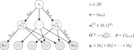
The proposed models belong to the broader family of Bayesian networks (Pearl, 2014), which are directed acyclic graphical models that can encode rich conditional independence information. We propose a ‘pyramid’-like Bayesian network with one latent variable at the root and more and more latent variables in downward layers, where the bottom layer consists of the observed variables . Denote the number of latent layers in this Bayesian network by , which can be viewed as the depth. Specifically, let the layer of latent variables consecutive to the observed be with variables, and let a deeper layer of latent variables consecutive to be for . Finally, at the top and the deepest layer of the pyramid, we specify a single discrete latent variable , or equivalently . In this Bayesian network, all the directed edges are pointing in the top-down direction only between two consecutive layers, and there are no edges between variables within a layer. This gives the following factorization of the joint distribution of and latent variables, where the subscript denotes an index of a random subject,
In the above display, for each , is a collection of first-latent-layer variables, which are parents of . Similarly, for each , is a collection of -latent-layer variables, which are parents of the -latent-layer variable .
Figure 1 gives a graphical visualization of the proposed model. To make clear the sparsity structure of this graph, we introduce binary matrices , termed as graphical matrices, to encode the connecting patterns between consecutive layers. That is, summarizes the parent–child graphical patterns between the two consecutive layers and . Specifically, matrix has size and matrix has size for , with entries
Each variable in the graph is subject-specific, implying that all the circles in Figure 1 represent subject-specific quantities. Namely, if there are subjects in the sample, each of them would have its own realizations of and s. The proposed directed acyclic graph is not necessarily a tree, as shown in Figure 1. That is, each variable can have multiple parent variables in the layer above it, while in a directed tree, each variable can only have one parent. As a simpler illustration, we also provide a two-latent-layer Bayesian Pyramid in Figure 2, which features a simpler yet still quite expressive architecture. For example, we can specify the conditional distribution of each observed using a multinomial or binomial logistic model with its parent variables as linear predictors and specify the distribution of given using a latent class model. Namely, for a random subject ,
Later in Section 4, we will focus on the two-latent-layer model when describing the estimation methodology; please refer to that part for further details.

Multiple layers of binary latent traits s model the distribution of observed . Binary matrices encode the sparse connection patterns between consecutive layers. Dotted arrows emanating from the root variable summarize omitted layers .
Two-latent-layer model. Latent variables and observed variables are subject-specific, and model parameters are population quantities.
We provide some discussions on the conceptual motivation for the proposed multilayer model. Intuitively, for each subject , in the deepest layer of the pyramid can encode some coarse-grained latent categories of subjects, while the vector encodes more fine-grained latent features of subjects. The hierarchical multilayer structure is conceptually appealing as it can provide latent representations of data in multiple resolutions, where there are nonlinear compositions between different latent resolutions that boost model flexibility. Model (3) for generating given is a nonlinear latent class model (LCM). Hence, cannot be viewed as a linear projection of the -layer; rather, the nonlinear LCM (with a deeper variable and conditional independence of ’s given ) can encode and explain rich and complex dependencies between the variables using parsimonious parametrizations.
2.2 Reformulating the Bayesian Pyramid as a constrained latent class model
In this subsection, we reveal an interesting equivalence relationship between our Bayesian Pyramid models and latent class models (LCMs, Goodman, 1974) with certain equality constraints. Such equivalence will pave the way for investigating the identifiability of Bayesian Pyramids. The traditional latent class model (LCM) (Goodman, 1974; Lazarsfeld, 1950) posits the following joint distribution of for a random subject :
The above equation specifies a finite mixture model with one discrete latent variable having categories (i.e., latent classes). In particular, given a latent variable , denotes the probability of belonging to the th latent class, and denotes the conditional probability of response for variable given the latent class membership . Expression (4) implies that observed variables are conditionally independent given the latent . In the Bayesian literature, the model in Dunson and Xing (2009) is a nonparametric generalization of (4), which allows an infinite number of latent classes.
Latent class modeling under (4) is widely used in social and biomedical sciences, where researchers often hope to infer subpopulations of individuals having different profiles (Collins & Lanza, 2009). However, the overly-simplistic form of (4) can lead to poor performance in inferring distinct and interpretable subpopulations. In particular, the model assumes that individuals in different subpopulations have completely different probabilities for all and , and conditionally on subpopulation membership all the variables are independent. These restrictions can force the number of classes to increase in order to provide an adequate fit to the data, which can degrade interpretability of a plain latent class model.
We introduce some notation before proceeding. Denote a all-one matrix by . For a matrix with rows and a set , denote by the submatrix of consisting of rows indexed in . Consider a family of constrained latent class models, which enable learning of a potentially large number of interpretable, identifiable, and diverse latent classes. A key idea is sharing of parameters within certain latent classes for each observed variable. We introduce a binary constraint matrix of size , which has rows indexed by the observed variables and columns indexed by the latent classes. The binary entry indicates whether the conditional probability table is free or instead equal to some unknown baseline. Specifically, if then is free; while for those latent classes such that , their conditional probability tables ’s are constrained to be equal. Hence, puts the following equality constraints on the parameters of (4):
We also enforce a natural inequality constraint for identifiability,
If , then there are no active constraints and the original latent class model (4) is recovered. We generally denote the conditional probability parameters by where if . As will be revealed soon, such constrained latent class models are related to our proposed Bayesian Pyramids via a neat mathematical transformation.
Viewed from a different perspective, a latent class model (4) specifies a decomposition of the -way probability tensor , where . This corresponds to the PARAFAC/CANDECOMP (CP) decomposition in the tensor literature (Kolda & Bader, 2009), which can be used to factorize general real-valued tensors, while our focus is on probability tensors. The proposed equality constraint (5) induces a family of constrained CP decompositions.
This family is connected with the sparse CP decomposition of Zhou et al. (2015), with both having equality constraints summarized by a binary matrix. However, Zhou et al. (2015) encourage different observed variables to share parameters, while our proposed model encourages different latent classes to share parameters through (5).
We have the following proposition linking the proposed multilayer Bayesian Pyramid to the constrained latent class model under equality constraint (5). For two vectors of the same length , denote if for all . Denote by the binary indicator function, which equals one if the statement inside is true and zero otherwise.
Consider the multilayer Bayesian Pyramid with binary graphical matrices .
In marginalizing out all the latent variables except, the distribution of is a constrained latent class model with latent classes, where each latent class can be characterized as one configuration of the -dimensional binary vector . The corresponding constraint matrix is determined by the bipartite graph structure between the -layer and the -layer, with entries being
(7)Further, in considering the distribution of and marginalizing out all the latent variables deeper than except, the distribution of is also a constrained latent class model with latent classes, where each latent class is characterized as one configuration of the -dimensional binary vector . Its corresponding constraint matrix is determined by the bipartite graph structure between the th and the th latent layers, with entries being
(8)
We present a toy example to illustrate Proposition 1 and discuss its implications.
Consider a multilayer Bayesian Pyramid with and , with the graph between and displayed in Figure 2. The graphical matrix is presented below. Proposition 1(a) states that there is a constraint matrix taking the form
Entries of are determined according to (7), for example, ; and . Each column of the constraint matrix is indexed by a latent class characterized by a configuration of a -dimensional binary vector. This implies that if only considering the first latent layer of variables , all the subjects are naturally divided into latent classes, each endowed with a binary pattern.
Proposition 1 gives a nice structural characterization of multilayer Bayesian Pyramids. This characterization is achieved by relating the multilayer sparse graph to the constrained latent class model in a layer-wise manner. This proposition provides a basis for investigating he identifiability of multilayer Bayesian Pyramids; see details in Section 3.
2.3 Connections to existing models and studies
We next briefly review connections between Bayesian Pyramids and existing models. In educational measurement research, Haertel (1989) first used the term restricted latent class models. Further developments along this line in the psychometrics literature led to a popular family of cognitive diagnosis models (de la Torre, 2011; Rupp & Templin, 2008; von Davier & Lee, 2019). These models are essentially binary latent skill models where each subject is endowed with a -dimensional latent skill vector indicating the mastery/deficiency statuses of skills, and each test item is designed to measure a certain configuration of skills, summarized by a loading vector . The matrix collecting all of the skill loading vectors as row vectors is often pre-specified by educational experts. The observed data for each subject are a -dimensional binary vector , indicating the correct/wrong answers to test questions in the assessment. Recently, there have been emerging studies on the identifiability and estimation of such cognitive diagnosis models (e.g., Chen, Culpepper, et al., 2020; Chen et al., 2015; Fang et al., 2019; Gu & Xu, 2019, 2020; Xu, 2017). However, to our knowledge, there have not been works that model multilayer (i.e., deep) latent structure behind the data and investigate identifiability in such scenarios.
Bayesian Pyramids are also related to deep belief networks (DBNs, Hinton et al., 2006), sum-product networks (SPNs, Poon & Domingos, 2011), and latent tree graphical models (LTMs, Mourad et al., 2013) in the machine learning literature. DBNs have undirected edges between the deepest two layers designed based on computational considerations (Hinton, 2009), while a Bayesian Pyramid is a fully generative directed graphical model (Bayesian network) with all the edges pointing top down. Such generative modeling is naturally motivated by the identifiability considerations and also provides a full description of the data generating process. Also, DBNs in their popular form are models for multivariate binary data, feature a fully connected graph structure, and use logistic link functions between layers. In contrast, Bayesian Pyramids accommodate general multivariate categorical data and allow flexible forms of layerwise conditional distributions and sparse connections between consecutive layers. An SPN is a rooted directed acyclic graph consisting of sum nodes and product nodes. Zhao et al. (2015) show that an SPN can be converted to a bipartite Bayesian network, where the number of discrete latent variables equals the number of sum nodes in the SPN. Our model is more general in that in addition to modeling a bipartite network between the latent layer and the observed layer, we further model the dependence of the latent variables instead of assuming them independent. LTMs are a special case of our model (3) because, while all the variables in an LTM form a tree, we allow for more general DAGs beyond trees. Although the above models are extremely popular, identifiability has received essentially no attention; an exception is Zwiernik (2018), which discussed identifiability for relatively simple LTMs.
Our two-latent-layer Bayesian Pyramid shares a similar structure with the nonparametric latent feature models in Doshi-Velez and Ghahramani (2009). Both works consider a mixture of binary latent feature models, with each data point associated with both a deep latent cluster ( in our notation) and a binary vector of latent features [ in our notation]. One distinction is that we adopt very flexible probabilistic distributions (see Examples 2 and 3) as conditional distributions in the DAG, while Doshi-Velez and Ghahramani (2009) posits that the latent features are a deterministic function of the products of and . In addition, Bayesian Pyramids are directly inspired by identifiability considerations, and in the next section, we provide explicit conditions that guarantee the model is identifiable—not only in the two-latent-layer architecture similar to Doshi-Velez and Ghahramani (2009) but also in general deep latent hierarchies with . Interestingly, Doshi-Velez and Ghahramani (2009) conjecture heuristically that their specification ‘likely resolves the identifiability issues’.
3 Identifiability and constrained latent class structure behind Bayesian Pyramids
3.1 Identifiability of the constrained latent class model and posterior consistency
In Section 2, we proposed a new class of multilayer latent variable models deemed Bayesian Pyramids and showed that these models can be formulated as a type of constrained latent class model (CLCM) defined in (4)–(5). In this section, we study theoretical properties of model (4)–(5).
The classic latent class model in (4) was shown by Gyllenberg et al. (1994) to be not strictly identifiable. Strict identifiability generally requires one to establish a parameterization in which the parameters can be expressed as one-to-one functions of observables. As a weaker notion, generic identifiability requires that the map is one-to-one except on a Lesbesgue measure zero subset of the parameter space. In a seminal paper, Allman et al. (2009) leveraged Kruskal’s theorem (Kruskal, 1977) to show generic identifiability for an unconstrained latent class model. However, Allman et al. (2009)’s approach is not sufficient for establishing identifiability in constrained LCMs or Bayesian Pyramids, due to the complex parameter constraints in these models. Indeed, Allman et al. (2009)’s generic identifiability results imply that in the latent class model with an unconstrained parameter space, there exists a measure-zero subset of parameters where identifiability breaks down. In constrained LCMs, the equality constraints (5) exactly enforce parameters to fall into a measure-zero subset. In Bayesian Pyramids, these equality constraints arise from between-layer potentially sparse graphs. So without a careful and thorough investigation into the relationship between the parameter constraints and the graphical structure, Kruskal’s theorem is not directly applicable to investigating the identifiability of constrained LCMs or Bayesian Pyramids.
Below, we establish strict identifiability of model (4)–(5), by carefully examining the algebraic structure imposed by the constraint matrix . We first introduce some notation. Denote by the Kronecker product of matrices and by the Khatri–Rao product of matrices. In particular, consider matrices , ; and matrices , , then there are and with
The above definitions show the Khatri–Rao product is a column-wise Kronecker product; see more in Kolda and Bader (2009). We first establish the following technical proposition, which is useful for the later theorem on identifiability.
For the constrained latent class model, define the following parameter matrices subject to constraints (5) and (6) with some constraint matrix ,
Denote the Khatri–Rao product of the above matrices by , which has size . The following two conclusions hold.
If the column vectors of the constraint matrix are distinct, then must have full column rank .
If contains identical column vectors, then can be rank-deficient.
Proposition 2 implies that having distinct columns is sufficient [in part (a)] and almost necessary [in part (b)] for the Khatri–Rao product to be full rank. To see the ‘almost necessary’ part, consider a special case where besides constraint (5) that if , the parameters also satisfy if . In this case, our proof shows that whenever the binary matrix contains identical column vectors in columns and , the matrix also contains identical column vectors in columns and and hence is surely rank-deficient.
In the Khatri–Rao product matrix defined in Proposition 2, each column characterizes the conditional distribution of vector given a particular latent class. Therefore, Proposition 2 reveals an nontrivial algebraic property: whether has distinct column vectors is linked to whether the conditional distributions of given each latent class are linearly independent. The matrix does not need to have full column rank in order to have distinct column vectors. For example, a matrix with three columns being , , and is rank-deficient but has distinct column vectors. Indeed, it is not hard to see that a binary matrix with rows can have as many as distinct column vectors.
Proposition 1 reformulates a Bayesian Pyramid into a constrained LCM with a constraint matrix , and then Proposition 2 establishes a nontrivial algebraic property of such constrained LCMs. Propositions 1 and 2 together pave the way for the development of the identifiability theory of Bayesian Pyramids. In particular, the sufficiency part of Proposition 2 uncovers a nontrivial inherent algebraic structure of the considered models. To prove Proposition 2, we leveraged a novel proof technique, the marginal probability matrix, in order to find a sufficient and almost necessary condition for the Khatri–Rao product of conditional probability matrices to have full rank. We anticipate that the conclusion in Proposition 2 can be useful in other graphical models with discrete latent variables, even beyond the Bayesian Pyramids considered in this paper. This is because graphical models involving discrete latent structure can often be formulated as a latent class model with equality constraints determined by the graph. Therefore, the conclusion of Proposition 2 might be of independent interest.
Although the linear independence of ’s columns itself does not lead to identifiability, it provides a basis for investigating strict identifiability of our model. We introduce the definition of strict identifiability under the current setup and then give the strict identifiability result.
Strict Identifiability
The constrained latent class model with (5) and (6) is said to be strictly identifiable if for any valid parameters , the following equality holds if and only if and are identical up to a latent class permutation:
When the constraint matrix is unknown and needs to be identified together with unknown continuous parameters , there is a trivial nonidentifiability issue that needs to be resolved. To see this, continue to consider the special case mentioned in Remark 1 where whenever , then given a matrix we can generally denote if and if . Then without further restrictions, the following alternative will be indistinguishable from the true , where , and . One straightforward way to resolve such trivial nonidentifiability of is to simply enforce that whenever the order of and is fixed for every possible category . In the following studies of identifiability, we always assume such orderings of with respect to has been fixed.
For an arbitrary subset , denote by the submatrix of that consists of those rows indexed by variables belonging to . has size .
Strict Identifiability
Consider the proposed constrained latent class model under (5) and (6) with true parameters , , and . Suppose there exists a partition of the variables such that
the submatrix has distinct column vectors for and ; and
for any , there is for some and some .
In the above theorem, the constraint matrix is not assumed to be fixed and known. This implies that both the matrix and the parameters can be uniquely identified from data. We next give a corollary of Theorem 1, which replaces the condition on parameters in part (b) with a slightly more stringent but also more transparent condition on the binary matrix .
Consider the proposed constrained latent class model under (5) and (6). Suppose for each . If there is a partition of the variables such that each submatrix has distinct column vectors for , then parameters are strictly identifiable up to a latent class permutation.
The conditions of Corollary 1 are more easily checkable than those in Theorem 1 because they only depend on the structure of the constraint matrix . It requires that after some column rearrangement, matrix should vertically stack three submatrices, each of which has distinct column vectors.
The conclusions of Theorem 1 and Corollary 1 both regard strict identifiability, which is the strongest possible conclusion on parameter identifiability up to label permutation. If we consider the slightly weaker notion of generic identifiability as proposed in Allman et al. (2009), the conditions in Theorem 1 and Corollary 1 can be relaxed. Given a constraint matrix , denote the constrained parameter space for by
and define the following subset of as
With the above notation, the generic identifiability of the proposed constrained latent class model is defined as follows.
Generic Identifiability
Parameters are said to be generically identifiable if defined in (11) has measure zero with respect to the Lebesgue measure on defined in (10).
Generic Identifiability
Consider the constrained latent class model under (5) and (6). Suppose for , changing some entries of from ‘’ to ‘’ yields an having distinct columns. Also suppose for any , there is for some and some . Then are generically identifiable.
Note that altering some from one to zero corresponds to adding one more equality constraint that the distribution of the th variable given the th latent class is set to the baseline through (5). Therefore, Theorem 2 intuitively implies that if enforcing more parameters in to be equal can give rise to a strictly identifiable model, then the parameters that make the original model unidentifiable only occupy a negligible set in .
Theorem 2 relaxes the conditions on for strict identifiability presented earlier. In particular, here the submatrices need not have distinct column vectors; rather, it would suffice if altering some entries of from one to zero yield distinct column vectors. As pointed out by Allman et al. (2009), generic identifiability is often sufficient for real data analyses.
So far, we have focused on discussing model identifiability. Next, we show that our identifiability results guarantee Bayesian posterior consistency under suitable priors. Given a sample of size , denote the observations by , which are vectors each of dimension . Recall that under (4), the distribution of the vector under the considered model can be denoted by a -way probability tensor . When adopting a Bayesian approach, one can specify prior distributions for the parameters , , and , which induce a prior distribution for the probability tensor . Within this context, we are now ready to state the following theorem.
Posterior Consistency
Denote the collection of model parameters by . Suppose the prior distributions for the parameters , , and all have full support around the true values. If the true latent structure and model parameters satisfy the proposed strict identifiability conditions in Theorem 1 or Corollary 1, we have
where is the complement of an -neighborhood of the true parameters in the parameter space.
Theorem 3 implies that under an identifiable model and with appropriately specified priors, the posterior distribution places increasing probability in arbitrarily small neighborhoods of the true parameters of the constrained latent class model as sample size increases. These parameters include the mixture proportions and the class specific conditional probabilities.
3.2 Identifiability of multilayer Bayesian Pyramids
According to Proposition 1, for a multilayer Bayesian Pyramid with a binary graphical matrix between the two bottom layers, one can follow (7) to construct a constraint matrix as illustrated in Example 1. We next provide transparent identifiability conditions that directly depend on the binary graphical matrices s. With the next theorem, one only needs to examine the structure of the between layer connecting graphs to establish identifiability.
Consider the multilayer latent variable model specified in (1)–(2). Suppose the numbers are known. Suppose each binary graphical matrix of size (size if ) takes the following form after some row permutation:
where generally denotes a submatrix of that can take an arbitrary form. Further suppose that the conditional distributions of variables satisfy the inequality constraint in (6). Then, the following parameters are identifiable up to a latent variable permutation within each layer: the probability distribution tensor for the deepest latent variable , the conditional probability table of each variable (including observed and latent) given its parents, and also the binary graphical matrices .
The proof of Theorem 4 provides a nice layer-wise argument on identifiability, that is, one can examine the structure of the Bayesian Pyramid in the bottom-up direction. As long as for some there are taking the form of (12), then the parameters associated with the conditional distribution of and are identifiable and the marginal distributions of are also identifiable.
Theorem 4 implies a requirement that and that for every , through the form of in (12). That is, the number of latent variables per layer decreases as the layer goes deeper up the pyramid. Condition (12) in Theorem 4 requires that each latent variable in the th latent layer has at least three children in the th layer that do not have any other parents. Our identifiability conditions hold regardless of the specific models chosen for the conditional distributions, and each , as long as the graphical structure is enforced and these component models are not over-parameterized in a naive manner. We next give two concrete examples which differently model the distribution of but both respect the graph given by .
We first consider modeling the effects of the parent variables of each as
where is a link function. The number of -parameters in (13) equals , which is the number of edges pointing to . Choosing leads to a model similar to sparse deep belief networks (Hinton et al., 2006; Lee et al., 2007).
To obtain a more parsimonious alternative to (13), let
Model (14) satisfies the conditional independence encoded by , since , implying that the distribution of only depends on its parents in the th latent layer. This model provides a probabilistic version of Boolean matrix factorization (Miettinen & Vreeken, 2014). The binary indicator equals the Boolean product of two binary vectors and . The and quantify the two probabilities that the entry does not equal the Boolean product.
Since Examples 2 and 3 satisfy the conditional independence constraints encoded by graphical matrices s, they satisfy the equality constraint in (5) with the constraint matrix . Therefore, our identifiability conclusion in Theorem 4 applies to both examples with appropriate inequality constraints on the —parameters or the —parameters; for example, see Proposition 3 in Section 4.
Besides Examples 2 and 3, there are many other models that respect the graphical structure. For example, (13) can be extended to include interaction effects of the parents of as follows:
In (15) if has parents, then the number of -parameters equals .
Anandkumar et al. (2013) considered the identifiability of linear Bayesian networks. Although both Anandkumar et al. (2013) and this work address identifiability issues of Bayesian networks, their results are not applicable to our highly nonlinear models. The nonlinearity requires techniques that look into the inherent tensor decomposition structures (in particular, a constrained CP decomposition) caused by the discrete latent variables and graphical constraints imposed on the discrete latent distribution. Such inherent constrained tensor structures are specific to discrete and graphical latent structures and are not present in the settings considered in Anandkumar et al. (2013).
4 Bayesian inference for two-layer Bayesian Pyramids
As discussed earlier, the proposed multilayer Bayesian Pyramid in Section 2 has universal identifiability arguments for many different model structures. In this section, as an important special case, we focus on a two-latent-layer model with depth and use a Bayesian approach to infer the latent structure and model parameters. Recall our two-latent-layer Bayesian Pyramid specified earlier in (3) takes the form
Here, we assume for all , as conventionally done in logistic models. The parameter can be viewed as the weight associated with the potential directed edge from latent variable to observed variable , for response category . The only impacts the likelihood if there is an edge from to with . Denote the collection of parameters as . (3) specifies a usual latent class model in the second latent layer with latent classes for the -dimensional latent vector . This layer of the model has latent class proportion parameters and conditional probability parameters . The full set of model parameters across layers is , and the model structure is shown in Figure 2. We can denote the conditional probability in (3) by .
4.1 Identifiability theory adapted to two-layer Bayesian Pyramids defined in (3)
For the two-latent-layer model in (3), the following proposition presents strict identifiability conditions in terms of explicit inequality constraints for the parameters.
Consider model (3) with true parameters .
Suppose , , , and for , . Then , , and probability tensor of are strictly identifiable.
Under the conditions of part (a), if further there is , then the parameters and are generically identifiable from .
As mentioned in the last paragraph of Section 2, the identifiability results in that section apply to general distributional assumptions for variables organized in a sparse multilayer Bayesian Pyramid. When considering specific models, properties of the model can be leveraged to weaken the identifiability conditions. The next proposition illustrates this, establishing generic identifiability for the model in (3). Before stating the identifiability result, we formally define the allowable constrained parameter space for under a graphical matrix as
Consider model (3) with belonging to in (16). Suppose the graphical matrix can be rewritten as , where each has size and
that is, each of has all the diagonal entries equal to one while any off-diagonal entry is free to be either one or zero. Also suppose . Then are generically identifiable.
The two different identifiability conditions on the binary graphical matrix stated in Propositions 3 and 4 correspond to different identifiability notions—strict and generic identifiability, respectively. The generic identifiability notion is slightly less stringent than strict identifiability, by allowing a Lebesgue-measure-zero subset of the parameter space where identifiability does not hold. Our sufficient generic identifiability conditions in Proposition 4 are much less stringent than conditions in Proposition 3.
4.2 Bayesian inference for the latent sparse graph and number of binary latent traits
We propose a Bayesian inference procedure for two-latent-layer Bayesian Pyramids. We apply a Gibbs sampler by employing the Polya-Gamma data augmentation in Polson et al. (2013) together with the auxiliary variable method for multinomial logit models in Holmes and Held (2006). Such Gibbs sampling steps can handle general multivariate categorical data.
4.2.1 Inference with a Fixed
First consider the case where the true number of binary latent variables in the middle layer is fixed. Inferring the latent sparse graph is equivalent to inferring the sparsity structure of the continuous parameters ’s. Let the prior for be , where hyperparameters can be set to give weakly informative priors for the logistic regression coefficients (Gelman et al., 2008). Specify priors for other parameters as
Here is a small positive number specifying the ‘pseudo’-variance, and we take in the numerical studies. Our adoption of a prior variance for when follows a similar spirit as the ‘pseudo-prior’ approach in the Bayesian variable selection literature. In Bayesian variable selection for regression analysis, Dellaportas et al. (2002) first proposed using a pseudo-prior for the variance when one variable is not included in the model to facilitate convenient Gibbs sampling steps. Specifically, a binary variable encodes whether or not the th predictor is included in the regression, and the regression coefficient is , with and . The pseudo-prior variance does not affect the posterior but may influence mixing of the MCMC algorithm.
The in (17) is further given a noninformative prior . The hyperparameters for the Inverse-Gamma distribution can be set to . In the data augmentation part, for each subject , each observed variable , and each non-baseline category , we introduce Polya-Gamma random variable . We use the auxiliary variable approach in Holmes and Held (2006) for multinomial regression to derive the conditional distribution of each . Given data , introduce binary indicators . The posteriors of satisfy that
and we introduce notation
Next by the property of the Polya-Gamma random variables (Polson et al., 2013), we have
where denotes the density function of PG. Based on the above identity, the conditional posterior of the ’s and ’s are still Gaussian, and the conditional posterior of each is still Polya-Gamma with ; these full conditional distributions are easy to sample from. As for the binary entries ’s indicating the presence or absence of edges in the Bayesian Pyramid, we sample each individually from its posterior Bernoulli distribution. The detailed steps of such a Gibbs sampler with known are presented in the Online Supplementary Material.
4.2.2 Inferring an Unknown
On top of the sampling algorithm described above for fixed , we propose a method for simultaneously inferring and other parameters. In the context of mixture models, Rousseau and Mengersen (2011) defined over-fitted mixtures with more than enough latent components and used shrinkage priors to effectively delete the unnecessary ones. In a similar spirit but motivated by Gaussian linear factor models, Legramanti et al. (2020) proposed the cumulative shrinkage process (CSP) prior, which has a spike and slab structure. We use a CSP prior on the variances of to infer the number of latent binary variables in a two-layer Bayesian Pyramid. The rationale for using such an increasing shrinkage prior for latent dimension selection is that, it is natural to expect additional latent dimensions to play a progressively less important role in characterizing the data, so the associated parameters should have a stochastically decreasing effect. Specifically, under the CSP prior, the th latent dimension is controlled by a scalar that follows a spike-and-slab distribution. Redundant dimensions will be essentially deleted by progressively shrinking the sequence towards an appropriate value (the spike). In particular, Legramanti et al. (2020) considered the continuous factor model where denotes the variance of the factor loadings for the th factor and is a small positive number indicating the variance of redundant latent factors.
We next describe in detail the prior specifications with an unknown number of binary latent variables . Consider an upper bound for , with . Based on the identifiability conditions in Theorem 4 about the shape of , is naturally constrained to be at most , therefore can be set to or smaller in practice. We adopt a prior that detects redundant binary latent variables by increasingly shrinking the variance of ’s as grows from 1 to . Specifically, letting , we put a CSP prior on variances for each category , where is a prespecified small positive number indicating the spike variance for redundant binary latent variables:
where refers to the inverse gamma distribution with shape and scale , and has a stick-breaking representation as in (20) with independently following the Beta distribution . We set to truncate the stick-breaking representation at , similarly to Legramanti et al. (2020). The represents the Dirac spike distribution with serving as the variance of redundant latent variables, while represents the more diffuse slab distribution for the variances corresponding to active latent variables. The ‘increasing shrinkage’ comes from the fact that as the latent variable index increases, the probability of belonging to the spike, , stochastically increases, because
increases as the index increases. Therefore, the CSP prior features an increasing amount of shrinkage for larger . We introduce auxiliary variables with to help with understanding and facilitate posterior computation. Specifically, the prior in (19) can be obtained by marginalizing out a discrete auxiliary variable with , so (19)–(20) can be reformulated in terms of as
Therefore, the auxiliary variables determine whether the th latent dimension is in the spike and hence corresponds to a redundant latent variable ; specifically, if then follows the slab distribution and is active, otherwise is in the spike and is redundant. Given (19), the largest possible number of active latent variables is , because and the last latent variable is always redundant. Since the event indicates that the th component is in the slab and hence active, we can write the total number of active latent dimensions as
Tracking the posterior samples of all the can give a posterior estimate of . The above data augmentation leads to Gibbs updating steps. We present the details of our Gibbs sampler in the Online Supplementary Material.
It is methodologically straightforward to extend our Gibbs sampler to deep Bayesian Pyramids with more than two latent layers. To see this, note that in deep Bayesian Pyramids with , for each , the conditional distribution of given in Example 2 is a special case of the conditional distribution of given . Indeed, both of these conditionals follow generalized linear models with the (multinomial) logit link, with the parent variables serving as predictors for the child. Under such a formulation, introducing additional Polya-Gamma auxiliary variables for the -layer similar to those for the -layer would allow Gibbs updates in a three-latent-layer Bayesian Pyramid. In this work, we focus on two-latent-layer models for computational efficiency.
We also remark that it is not hard to derive and implement a Gibbs sampler for constrained latent class models (CLCMs) mentioned in Section 3.1. Performing Gibbs sampling for CLCMs is a relatively straightforward extension to the current Gibbs sampler for Bayesian Pyramids. The reason is that one can similarly use the data augmentation strategies in Holmes and Held (2006) and Polson et al. (2013) to deal with ; and one can also adopt similar priors for the binary constraint matrix as those adopted for the graphical matrix in a Bayesian Pyramid. Our preliminary simulations for such a Gibbs sampler under CLCMs showed that the recovery of parameters and the constraint matrix are not as stable and accurate as that for Bayesian Pyramids (shown in the later Figures 3–5). One explanation is that compared to multilayer Bayesian Pyramids, the parametrization of a CLCM is less parsimonious and requires many more mixture proportion parameters in order to describe the same joint distribution of the observed variables. Therefore, we have chosen to focus on the method for Bayesian Pyramids in this work, and treat CLCMs mainly as intermediate tools to help establish identifiability of Bayesian Pyramids.
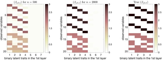
Posterior means of the main-effect parameters for response category averaged across 50 independent replications, for or . is taken in the CSP prior for posterior inference, while the true is 4 as shown in the rightmost plot.
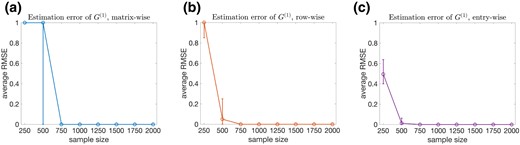
Mean estimation errors of the binary graphical matrix at the matrix level (in (a)), row level (in (b)), and entry level (in (c)). The median, 25% quantile, and 75% quantile based on the 50 independent simulation replications are shown by the circle, lower bar, and upper bar, respectively.
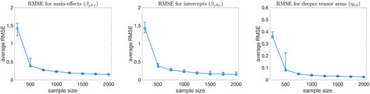
Average root-mean-square errors (RMSE) of the posterior means of the main-effects , intercepts , and deeper tensor arms versus sample size for . The median, 25% quantile, and 75% quantile based on the 50 independent simulation replications are shown by the circle, lower bar, and upper bar, respectively.
5 Simulation studies
We conducted replicated simulation studies to assess the Bayesian procedure proposed in Section 4 and examine whether the model parameters are indeed estimable as implied by Theorem 3. Consider a two-latent-layer Bayesian Pyramid with observed variables, response categories for each observed variable, and binary latent variables in the middle layer and one binary latent variable in the deep layer. Let the true binary graphical matrix be . Such a satisfies the conditions for strict identifiability in Theorem 4, since it contains three copies of the identity matrix as submatrices. Let the true intercept parameters for categories be for each ; and for any , let the corresponding true main-effect parameters of the binary latent variables be if variable has a single parent and if has multiple parents. See Figure 3c for a heatmap of the sparse matrix of the main-effect parameters for category .
We use the method developed in Section 4 with the CSP prior for posterior inference under an unknown . We specify an upper bound for as , because is a natural upper bound here based on the identifiability considerations mentioned before. As for the hyperparameters in the CSP prior, we mainly follow the default setting and suggestion in Legramanti et al. (2020). Specifically, we set to the same value in Legramanti et al. (2020), ; we also follow the suggestion in Legramanti et al. (2020) that the spike variance should be a small positive number but should avoid to take excessively low values by setting . Our simulations adopting these choices turn out to produce accurate estimation results under different settings (see the later Figures 3–5). In our preliminary simulations, we also varied these hyperparameters around the above values, and did not observe the algorithmic performance to be sensitive to them. Throughout the Gibbs sampling iterations, we enforce an identifiability constraint on that as long as . For each sample size we conduct 50 independent simulation replications. Since the model is identifiable up to a permutation of the latent variables in each layer, we post-process the posterior samples to find a column permutation of to best match the simulation truth; then the columns of other parameter matrices are permuted accordingly.
We have used the Gelman-Rubin convergence diagnostic (Gelman et al., 2013; Gelman & Rubin, 1992) to assess the convergence of the MCMC output from multiple random initializations. In particular, for the simulation setting corresponding to , we randomly initialize the parameters from their prior distributions times and then run five MCMC chains for each simulated dataset. For each MCMC chain, we ran the chain for 15,000 iterations, discarding the first 10,000 iterations as burn-in, and retaining every fifth sample post burn-in to thin the chain. After collecting the posterior samples, we calculate the potential scale reduction factor (i.e., the Gelman-Rubin statistic) of the model parameters. The median Gelman-Rubin statistics for the deep conditional probabilities and that for the deep latent class proportions across the five chains are as follows:
The Gelman–Rubin statistics for other parameters are similarly well controlled and are omitted. We also inspected the traceplots of the MCMC outputs and observed fast mixing of the MCMC chain after convergence. These observations justify running MCMC for 15,000 iterations and discarding the first 10,000 as burn-in, therefore we adopt these settings in all the numerical experiments. When applying the proposed method to other datasets, we also recommend calculating the Gelman–Rubin statistics and inspecting the traceplots to determine the appropriate number of overall MCMC iterations and burn-in iterations.
Our Bayesian modeling of adopts rather uninformative priors with each entry and we do not force to take a specific form (such as to include any identity submatrix as described in Proposition 3 for strict identifiability) but rather let the sampler freely explore the space of all binary matrices to estimate . Our theory on identifiability and posterior consistency implies that the posteriors of both and other parameters concentrate around their true values as sample size grows. This is empirically verified in our simulation studies; Figures 3–5 show that as sample size grows, both the discrete and the continuous parameters are estimated consistently. We next elaborate on these findings from simulations.
Figure 3 presents posterior means of the main-effect parameters for category , averaged across the 50 independent replications. The leftmost plot of Figure 3 shows that for a relatively small sample size , the posterior means of already exhibit similar structure as the ground truth in the rightmost plot. Also, the true number of binary latent variables in the middle latent layer are revealed in Figures 3a and b. For the sample size , Figure 3b shows that the posterior means of are very close to the ground truth. The posterior means for other categories show similar patterns to those for . The estimated are slightly biased toward zero for the smaller sample size () with bias less for the larger sample size (). Our results suggest that the binary graphical matrix that underlies (that is, the sparsity structure of the continuous parameters) is easier to estimate than the nonzero themselves. That is, with finite samples, the existence of a link between each observed variable and each binary latent variable is easier to estimate than the strength of such a link (if it exists).
To assess how the approach performs with an increasing sample size, we consider eight sample sizes for under the same settings as above. To compare the estimated structures to the simulation truth with , we retain exactly four binary latent variables ; choosing those having the largest average posterior variance . For the discrete structure of the binary graphical matrix , we present mean estimation errors in Figure 4. Specifically, Figure 4a plots the errors of recovering the entire matrix , Figure 4b plots the errors of recovering the row vectors of , and Figure 4b plots the errors of recovering the individual entries of . For sample size as small as , estimation of is very accurate across the simulation replications. Notably, is much smaller than the total number of cells in the contingency table for the observed variables . For continuous parameters , , and , respectively, in Figure 5 we plot average root-mean-square errors (RMSE) of the posterior means versus sample size . For each , , and , Figure 5 shows RMSE decreases with sample size, which is as expected given our posterior consistency result in Theorem 3.
In simulations (and also the later real data analysis), we have checked the posterior samples collected from the MCMC algorithm and obtained the traceplots of various parameters in the model. By examining these, we have not observed label-switching issues in our numerical studies. In general, we would suggest one uses the traceplots of those mixture-component-specific parameters to examine whether there is a label switching issue. If there exists such issues, we recommend using the R package label.switching (Papastamoulis, 2016) for MCMC outputs to address the issue.
6 Application to DNA nucleotide sequence data
We apply our proposed two-latent-layer Bayesian Pyramid with the CSP prior to the Splice Junction dataset of DNA nucleotide sequences; the data are available from the UCI machine learning repository. We also analyze another dataset of nucleotide sequences, the Promoter data, and present the results in the Online Supplementary Material. The Splice Junction data consist of A, C, G, T nucleotides () at positions for DNA sequences. There are two types of genomic regions called introns and exons; junctions between these two are called splice junctions (Nguyen et al., 2016). Splice junctions can be further categorized as (a) exon-intron junction; and (b) intron-exon junction. The samples in the Splice dataset each belong to one of three types: Exon-Intron junction (‘EI’, 762 samples); Intron-Exon junction (‘IE’, 765 samples); and Neither EI or IE (‘N’, 1648 samples). Previous studies have used supervised learning methods for predicting sequence type (e.g., Li & Wong, 2003; Nguyen et al., 2016). Here we fit the proposed two-latent-layer Bayesian Pyramid to the data in a completely unsupervised manner, with the sequence type information held out. We use the nucleotide sequences to learn discrete latent representations of each sequence, and then investigate whether the learned lower dimensional discrete latent features are interpretable and predictive of the sequence type.
We let the variable in the deepest latent layer have categories, inspired by the fact that there are three types of sequences: EI, IE, and N; but we do not use any information of which sequence belongs to which type when fitting the model to data. As mentioned earlier, the upper bound for the binary latent variables can be set to or smaller in order to yield an identifiable Bayesian Pyramid model. In practice, when is large, we recommend starting with a relatively small , inspecting the estimated active/redundant latent dimensions, and only increasing if all the latent dimensions are estimated to be active a posteriori (that is, if the posterior model of defined in (21) equals ). For this splice junction dataset with , we start with for better computational efficiency; this is the same as that used in the simulations and already allows for distinct latent binary profiles. We find that the posteriors select only active latent dimensions; this suggests that it is not necessary to increase to a larger number for this dataset.
We still run the Gibbs sampler for 15,000 iterations, discarding the first 10,000 as burn-in, and retaining every fifth sample post burn-in to thin the chain. Based on examining traceplots, the sampler has good mixing behavior. As mentioned in the last paragraph, our method selects binary latent variables. We index the saved posterior samples by , for each denote the samples of by . Similarly for each , denote the posterior samples of the nucleotides sequences’ latent binary traits by , and denote those of the nucleotide sequences’ deep latent category by where . Define our final estimators , , and to be
, , and summarize information of the element-wise posterior modes of the discrete latent structures in our model. The matrix depicts how the loci load on the binary latent traits, the matrix depicts the presence or absence of each binary latent trait in each nucleotide sequence, and the matrix depicts which deep latent group each nucleotide sequence belongs to. , , and are all binary matrices, but the first two are binary feature matrices while the last one has each row having exactly one entry of ‘1’ indicating group membership. In Figure 6, the first three plots display the three estimated matrices , , and , respectively; and the last plot shows the held-out gene type information for reference. As for the estimated loci loading matrix , Figure 6a provides information on how the loci depend on the five binary latent traits. Specifically, we found that the first 27 loci show somewhat similar loading patterns and mainly load on the first four binary traits. Also, the middle 10 loci (from locus 28 to locus 37) are similar in loading on all five traits, and the last 23 loci (from locus 38 to locus 60) are similar in exhibiting sparser loading structures. Figure 6b–d shows that the two matrices and corresponding to the nucleotide sequences exhibit a clear pattern of clustering, which aligns well with the known but held-out junction types EI, IE, and N.
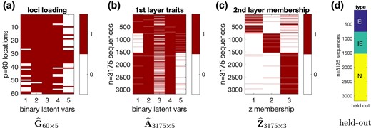
Splice junction data analysis under the CSP prior with . Plots are presented with the binary latent traits selected by our proposed method a posteriori. After applying the rule-lists approach to deterministically match the latent features to the gene types as in (22), the accuracies for predicting the gene types EI, IE, N are all above 95%.
To formally assess how the latent discrete features learned by the proposed method perform in downstream prediction, we apply the ‘rule lists’ classification approach in Angelino et al. (2017) to the estimated latent features in and for nucleotide sequences. The rule-lists approach is an interpretable classification method based on a categorical feature space, and it finds simple and deterministic rules of the categorical features in predicting a (binary) class label. For each instance , we define the categorical features to be the eight-dimensional vector . is concatenated from and and is a feature vector of binary entries. Denote the ground-truth nucleotide sequence types by , then for , for , and for . Recall that the information of ’s are not used in fitting our Bayesian Pyramid to obtain the latent features ’s. We use the Python package CORELS for the rule-lists method with ’s and ’s as input, and find rules that match ’s to ’s. Specifically, these deterministic rules given by CORELS are:
Equation (22) gives a very simple and explicit rule depending on , , and for each nucleotide sequence . This simple rule can be empirically verified by comparing the middle two plots to the rightmost plot in Figure 6. In (22), the rules for EI and IE are not mutually exclusive, but those for EI and N are mutually exclusive and the same holds for IE and N. Therefore, to obtain mutually exclusive rules for the three class labels EI, IE, and N based on (22), we can simply define the following two types of labels and :
For the two types of labels and in (23), we provide their corresponding normalized confusion matrices in Figure 7 along with their heatmaps. Figure 7 shows that both and have very high prediction accuracies for the sequence types , with all the diagonal entries above . The superb prediction performance as shown in Figure 7 implies that the learned discrete latent features of nucleotide sequences are interpretable and very useful in the downstream task of classification. For the Splice Juntion dataset, such accuracies are even comparable to the state-of-the-art prediction performance given by fine-tuned convolutional neural networks given in Nguyen et al. (2016), which are also between 95% and 97%.
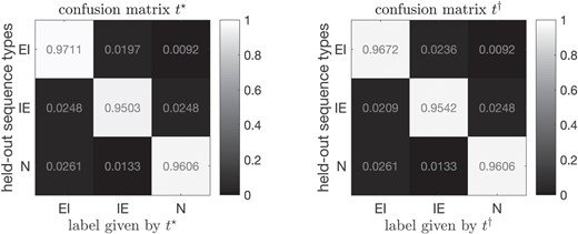
Downstream interpretable classification results for splice junction data following fitting the two-latent-layer Bayesian Pyramid. Prediction performance of the learned lower-dimensional discrete latent features are summarized in two confusion matrices, corresponding to and defined in (23).
In the above data analysis, we have fixed inspired by the fact that there are three types of splice junctions. Alternatively, we can use the overfitted mixture framework of Rousseau and Mengersen (2011) to accommodate an unknown . Overfitted mixtures are finite mixture models with an unknown number of mixture components , where only an upper bound of is known. In such scenarios, Rousseau and Mengersen (2011) proposed to use shrinkage priors for the mixture proportion parameters, such as Dirichlet priors with small Dirichlet hyperparameters. More specifically, denote the mixture proportion parameters corresponding to the ‘overfitted’ mixture components by , then lives on the -dimensional probability simplex. The overfitted mixture framework in Rousseau and Mengersen (2011) guarantees that with the prior where the Dirichlet parameters are small enough with respect to the dimension of the observations, the redundant mixture components will be ‘emptied out’ in the posterior asymptotically. Hence, the true mixture components underlying the data will be identified from the posterior distribution. In the Online Supplementary Material, we reanalyze the real data specifying and simulation studies with an overfitted , and achieve favorable results.
For comparison, we also applied/implemented two alternative discrete latent structure models, including: (a) the latent class model, with a single univariate discrete latent variable behind the observed data layer; and (b) a single-latent-layer model, with one layer of independent binary latent variables behind the data layer. For model (a), we applied the nonparametric Bayesian method in Dunson and Xing (2009) to the splice junction dataset and extracted latent classes (default in Dunson & Xing, 2009; increasing beyond 10 is not considered because in the current 10 latent classes there are already empty classes not occupied by any nucleotide sequence). For model (b), we implemented a new Gibbs sampler (see description in Section 9.3 in the Online Supplementary Material), still employing the cumulative shrinkage process prior as used for Bayesian Pyramids. Then based on the learned lower-dimensional latent representations, we still apply the ‘rule-lists’ classification approach in Angelino et al. (2017) (via the Python package CORELS) for each of the three labels EI, IE, and N via binary classification. In addition to the above two competitors (abbreviated as ‘DX2009’ and ‘IndepBinary’, respectively), we also consider a benchmark approach of directly applying the rule-lists classifier to raw DNA nucleotide sequences. Since the rule-lists classifier in the CORELS package only applies to binary predictors, we first convert the DNA nucleotide sequences of A, G, C, T into longer sequences containing binary indicators of whether each loci is ‘A’, or ‘G’, or ‘C’; after this, each original -dimensional nucleotide sequence is converted to a binary vector of length . We then apply the rule-lists classifier using the same setting of learning at most three ‘rules’ (i.e., in the CORELS package) as all the other three latent variable methods: DX2009, IndepBinary, and BayesPyramid. We obtain the classification accuracy in Table 1.
Downstream classification accuracy for splice data
| EI (train) | IE (train) | N (train) | EI (test) | IE (test) | N (test) | |
|---|---|---|---|---|---|---|
| Raw nucleotide nucleotides | 0.909 | 0.854 | 0.840 | 0.916 | 0.866 | 0.839 |
| DX2009 | 0.946 | 0.955 | 0.918 | 0.950 | 0.965 | 0.929 |
| IndepBinary | 0.964 | 0.955 | 0.956 | 0.965 | 0.957 | 0.965 |
| BayesPyramid | 0.971 | 0.975 | 0.970 | 0.984 | 0.983 | 0.976 |
The left three columns in Table 1 list accuracies on the training set containing 80% of the samples, and the right three columns on the test set containing the remaining 20% of the samples. The test accuracies are very close to the training ones, indicating satisfactory generalizability. The reason is that the maximum number of rules learned for each model is limited to be at most three, i.e., in the CORELS package. Such a small number of rules in a classifier do not overfit the training data and hence generalize well to the test data. We remark that when increasing max_card beyond three, the downstream classification accuracy of BayesPyramid remains the same as those in Table 1; however, for the raw nucleotide sequences, the CORELS package cannot complete the execution of the classifier with , likely due to the high-dimensionality of the search space of rules. Therefore, we present the results of CORELS classification with in Table 1.
Remarkably, Table 1 shows that all the three unsupervised learning methods learn latent features that are more predictive of the sequence type than the raw sequences themselves, among which the Bayesian Pyramid is the apparent top performer. This observation indicates that the latent variable approaches, especially our multilayer Bayesian Pyramids, can ‘denoise’ the raw sequence data and return more useful features for downstream tasks. The model in Dunson and Xing (2009) (‘DX2009’) and the single-layer-independent-latent model (‘IndepBinary’) are special cases of Bayesian Pyramids, and both have excellent performance on the splice data. However, Bayesian Pyramids significantly decreased the test set misclassification rate of IndepBinary by 31%–60%, of DX2009 by 51%–68%, and of raw nucleotide sequences by 81%–87%.
7 Discussion
In this article, we have proposed Bayesian Pyramids, a general family of discrete multilayer latent variable models for multivariate categorical data. Bayesian Pyramids cover multiple existing statistical and machine learning models as special cases, while allowing for various different assumptions on the conditional distributions. Our identifiability theory is key in providing reassurance that one can reliably and reproducibly learn the latent structure, guarantees that are lacking from almost all of the related literature. The proposed Bayesian approach has excellent performance in the simulations and data analyses, and shows good computational performance and a surprising ability to accurately infer meaningful and useful latent structure. There are immediate applications of the proposed Bayesian Pyramid approach in many other disciplines. For example, in ecology and biodiversity research, joint species distribution modeling is a very active area (see a recent book of Ovaskainen & Abrego, 2020). The data consist of high-dimensional binary indicators of presence or absence of different species at each sampling location. In this contest, Bayesian Pyramids provide a useful approach for inferring latent community structure of biologic and ecological interest.
This work focuses on the unsupervised setting and uses latent variable approaches. In unsupervised cases, there is not a specific outcome/response associated with each data point, and the general goal is to discover ‘interesting’ patterns in data (Murphy, 2012). Such unsupervised learning problems are generally considered more challenging and less well studied than supervised ones. Latent variables can capture semantically interpretable constructs, and marginalizing out latents induces great flexibility in the resulting marginal distribution of observables. Bayesian Pyramids provide unsupervised feature discovery tools for learning latent architectures underlying multivariate data, yielding insight into data generating processes, performing nonlinear dimension reduction, and extracting useful latent representations.
In order to realize the great potential of latent variable approaches to unsupervised learning, identifiability issues must be addressed so that reliable latent constructs can be reproducibly extracted from data. Especially, if one wishes to interpret the latent representations and parameters estimated from a latent variable model and use them in downstream analyses, then identifiability is a prerequisite for making such interpretation meaningful and reproducible. In this sense, identifiability is necessary for interpretability of the latent structures. We remark that such interpretability considerations differ from the goals of learning interpretable treatment rules for some outcome in complex supervised learning settings (see, e.g., Kitagawa & Tetenov, 2018; Semenova & Chernozhukov, 2021). In modern machine learning, although powerful deep latent variable models have been proposed, identifiability issues have rarely been considered and the design of the latent architecture is often guided by heuristics. In this work, our identifiability theory directly inspires how to specify the deep latent architecture in a Bayesian Pyramid: the identifiability conditions on matrices (in Theorem 4) inspire us to specify a ‘pyramid’ structure featuring fewer and fewer latent variables deeper up the hierarchy () and sparse graphical connections between layers.
In the future, it is worth further advancing and refining scalable algorithms for Bayesian Pyramids beyond the two-latent-layer case. Methodologically, our current Gibbs sampling procedure can be readily extended to multiple latent layers, because non-adjacent layers in a Bayesian Pyramid are conditionally independent and the current Gibbs updates for shallower layers can be similarly applied to deeper ones. In terms of the computational performance, however, efficiently sampling discrete latent variables via MCMC is generally more challenging than sampling continuous ones. In a Bayesian Pyramid, binary entries of the graphical matrices act similarly as covariate selection indicators in (logistic) regression problems, yet are more difficult to estimate because the ‘covariates’ themselves are latent and discrete. This fact can cause unsatisfactory mixing behavior of naive extensions of the Gibbs sampler to deeper models. For example, sampling to update an entry in a deeper graphical matrix where can cause a substantial shift of the posterior space for the associated continuous parameters in downward layers. Future research is warranted to advance the MCMC methodology or explore complementary methods for estimating the discrete latent structures in deeper models.
Acknowledgments
The authors thank the Editor, Associate Editor, and three referees for helpful and constructive comments.
Funding
This work was partially supported by the National Science Foundation grant DMS-2210796. This work was also partially supported by grants R01ES027498 and R01ES028804 from National Institutes of Environmental Health Sciences of the National Institutes of Health, and received funding from European Research Council under the European Union’s Horizon 2020 research and innovation program (grant agreement No 856506).
Data availability
Matlab code implementing the proposed method and data are available at this GitHub repository: https://github.com/yuqigu/BayesianPyramids.
Supplementary material
Supplementary material are available at Journal of the Royal Statistical Society: Series B online.
References
Author notes
Conflict of interest None declared.
