


Abstract
Estimating dynamic treatment regimes (DTRs) from retrospective observational data is challenging as some degree of unmeasured confounding is often expected. In this work, we develop a framework of estimating properly defined ‘optimal’ DTRs with a time-varying instrumental variable (IV) when unmeasured covariates confound the treatment and outcome, rendering the potential outcome distributions only partially identified. We derive a novel Bellman equation under partial identification, use it to define a generic class of estimands (termed IV-optimal DTRs) and study the associated estimation problem. We then extend the IV-optimality framework to tackle the policy improvement problem, delivering IV-improved DTRs that are guaranteed to perform no worse and potentially better than a prespecified baseline DTR. Importantly, this IV-improvement framework opens up the possibility of strictly improving upon DTRs that are optimal under the no unmeasured confounding assumption (NUCA). We demonstrate via extensive simulations the superior performance of IV-optimal and IV-improved DTRs over the DTRs that are optimal only under the NUCA. In a real data example, we embed retrospective observational registry data into a natural, two-stage experiment with noncompliance using a differential-distance-based, time-varying IV and estimate useful IV-optimal DTRs that assign mothers to a high-level or low-level neonatal intensive care unit based on their prognostic variables.
1 Introduction
1.1 Dynamic treatment regime and instrumental variable
Estimating single-stage individualized treatment rules (ITRs) and the more general multiple-stage dynamic treatment regimes (DTRs) has attracted a lot of interest from diverse disciplines. Many estimation strategies have been proposed in the literature for data derived from randomized controlled trials or observational databases. Two main strands of work are Q-learning based on positing regression models for the outcome of interest at each stage based on study participants’ information and A-learning based on modelling the contrasts among treatments. Both methods can further be combined with classification tools to yield more robust and interpretable decision rules. Important examples of these methodologies include Murphy et al. (2001), Murphy (2003), Robins (2004), Chakraborty et al. (2010), Rubin and van der Laan (2012), Zhao et al. (2012), Zhao et al. (2015), Laber and Zhao (2015), Zhou et al. (2017), Tao et al. (2018), Zhang et al. (2018), Zhang and Zhang (2018), and Athey and Wager (2020), among many others. For a more comprehensive review of various methods, see, e.g., Moodie et al. (2007), Chakraborty and Murphy (2014), and Schulte et al. (2014).
Estimating optimal policies (ITRs or DTRs) can be challenging when data comes from observational databases (e.g., Medicare and Medicaid claims database, disease registry, etc) where some degree of unmeasured confounding is always expected. In these scenarios, an instrumental variable (IV) is a useful tool to infer the treatment effect (Angrist et al., 1996). An instrumental variable is valid if it is associated with the treatment (IV relevance), affects the outcome only through its association with the treatment (exclusion restriction) and is independent of the unobserved treatment-outcome confounding variables, possibly conditional on a rich set of observed covariates (IV unconfoundedness). We will rigorously define these IV identification assumptions in Section 2.
One subtlety in IV-based analyses is that even a valid IV cannot always identify the mean potential outcomes; rather, a valid IV along with appropriate, application-specific identification assumptions places certain restrictions on the potential outcome distributions, and this line of research is known as partial identification of probability distributions (Manski, 2003). This subtlety is inherited by the policy estimation problem using an IV. In particular, when the conditional average treatment effect (CATE) is not point identified from data, the optimal policy that maximizes the value function cannot be identified either, necessitating researchers to target alternative optimality criteria. While such criteria have been proposed in the single-stage setting from different perspectives (Cui & Tchetgen Tchetgen, 2020, 2021; Pu & Zhang, 2021), literature on the more general, multiple-stage setting is scarce.
Our first contribution in this article is to generalize the optimality criteria in the single-stage setting and develop a framework that is tailored to general sequential decision-making problems and incorporates rich information contained in a time-varying IV. This optimality criterion, termed IV-optimality, is based on a carefully weighted version of the partially identified Q-function and value function subject to the distributional constraints imposed by the IV. This criterion is distinct from the framework of Han (2019) that endows the collection of partially identified DTRs with a partial order and characterizes the set of maximal elements (see Zhang et al., 2020 for similar ideas). It is also distinct from Liao et al. (2021) that models the transition dynamics and assumes that the unmeasured treatment-outcome confounder is additive and not an effect modifier itself at any stage, or Shi et al. (2022) that utilizes Pearl’s (2009) ‘front-door criterion’ to aid point identification of optimal DTR in the presence of unmeasured treatment-outcome confounding. In the current work, we do not impose, a priori, assumptions that induce point identification. Importantly, our proposed set of optimality criteria collapse to that targeted by Liao et al. (2021) if the time-varying IV point identifies the treatment effect under an additional ‘additive unmeasured confounding’ assumption studied in Liao et al. (2021) and more general point-identification assumptions proposed and reviewed in Frangakis and Rubin (1999), Hernán and Robins (2006), Wang and Tchetgen Tchetgen (2018), and Swanson et al. (2018, Section 5). We take a hybrid approach of Q-learning (Schulte et al., 2014; Watkins & Dayan, 1992) and weighted classification (Zhang et al., 2012; Zhao et al., 2012) to target this optimality criterion and establish nonasymptotic rate of convergence of the proposed estimators.
The IV-optimality framework also motivates a conceptually simple yet informative variant framework that allows researchers to leverage a time-varying IV to improve upon a baseline DTR. The policy improvement problem was first considered in a series of papers by Kallus et al. (2019) and Kallus and Zhou (2020a, 2020b) under a ‘Rosenbaum-bounds-type’ sensitivity analysis model (Rosenbaum, 2002b). Despite its novelty and usefulness in a range of application scenarios, a sensitivity-analysis-based policy improvement framework does have a few limitations. In particular, each improved policy is indexed by a sensitivity parameter Γ that controls the degree of unmeasured confounding. Since the sensitivity parameter is not identified from the observed data, it is often unclear which improved policy best serves the purpose. Moreover, ‘Rosenbaum-bounds-type’ sensitivity analysis model does not fully take into account unmeasured confounding heterogeneity (Bonvini & Kennedy, 2021; Heng & Small, 2020). On the contrary, an IV-based policy improvement framework outputs data-driven partial identification intervals that are not indexed by sensitivity parameters. Additional information contained in the IV also opens up the possibility of strictly improving upon a policy that is optimal under the no unmeasured confounding assumption (NUCA) (Robins, 1992; Rosenbaum & Rubin, 1983), when the NUCA is in fact violated.
Our proposed method has two important applications. First, it is applicable when empirical researchers want to estimate useful DTRs from noisy observational data and have access to a time-varying IV at each stage, e.g., daily precipitation, differential distance, etc. Second, the framework described here is central to many sequential multiple assignment randomized trial (SMART) designs (Murphy, 2005) where interest lies in comparing adaptive interventions, and patients assigned to a particular treatment at each stage may not adhere to it. Noncompliance makes the treatment assigned at every stage a valid time-varying IV, and our proposed method provides a principled way to account for systematic noncompliance in SMART designs.
The rest of the article is organized as follows. We describe a real data application in Section 1.2. Section 2 reviews optimality criteria in the single-stage setting and provides a general IV-optimality framework that is amenable to being extended to the multiple-stage setting. Section 3 considers improving upon a baseline ITR with an IV. Building upon Sections 2 and 3, we describe an IV-optimality framework for policy estimation in the multiple-stage setting and extend this framework to tackle the policy improvement problem in Section 4. Section 5 studies the theoretical properties of the proposed methods. We report simulation results in Section 6 and revisit the application in Section 7. Section 8 concludes with a brief discussion. For brevity, all proofs are deferred to the Online Supplemental Materials S2 and S3.
1.2 Application: a natural, two-stage experiment derived from registry data
Lorch et al. (2012) conducted a retrospective cohort study to investigate the effect of delivery hospital on premature babies (gestational age between 23 and 37 weeks) and found a significant benefit to neonatal outcomes when premature babies were delivered at hospitals with high-level neonatal intensive care units (NICUs) compared to those without high-level NICUs. Lorch et al. (2012) used the differential travel time to the nearest high-level versus low-level NICU as an IV so that the outcome analysis is less confounded by mothers’ self-selection into hospitals with high-level NICUs. In their original study design, Lorch et al. (2012) further controlled for mothers’ neighbourhood characteristics, as well as their demographic information and variables related to delivery, in their matching-based study design so that the differential travel time was more likely to be a valid IV conditional on these variables. Put another way, the differential travel time created a natural experiment with noncompliance: Similar mothers who lived relatively close to a hospital with high-level NICUs were encouraged (but not forced) to deliver at a high-level NICU. More recently, Michael et al. (2020) considered mothers who delivered exactly two babies from 1996 to 2005 in Pennsylvania and investigated the cumulative effect of delivering at a high-level NICU on neonatal survival probability using the same differential travel time IV.
Currently, there is still limited capacity at high-level NICUs, so it is not practical to direct all mothers to these high-technology, high-volume hospitals. Understanding which mothers would most significantly benefit from delivering at a high-level NICU helps design optimal perinatal regionalization systems that designate hospitals by the scope of perinatal service provided and designate where infants are born or transferred according to the level of care they need at birth (Kroelinger et al., 2018; Lasswell et al., 2010). Indeed, previous studies seemed to suggest that although high-level NICUs significantly reduced deaths for babies of small gestational age, they made little difference for almost mature babies like 37 weeks (Yang et al., 2014).
Mothers who happened to relocate during two consecutive deliveries of babies constitute a natural two-stage, two-arm randomized controlled trial with noncompliance and present a unique opportunity to investigate an optimal DTR. See Figure 1 for the directed acyclic graph (DAG) illustrating this application. We will revisit the application after developing a methodology precisely suited for this purpose.

A DAG illustrating the NICU application. Observed baseline covariates like mothers’ demographics, neighbourhood characteristics, etc., are omitted for clearer presentation.
2 Estimating individualized treatment rules with an instrumental variable
2.1 Optimal and NUCA-optimal ITRs
We first define the estimand of interest, an optimal ITR, under the potential outcome framework (Neyman, 1923; Rubin, 1974) and briefly review how to estimate the optimal ITR under the NUCA.
Consider a single-stage decision problem where one observes the covariates , takes a binary action and receives the response . Here, denotes the potential outcome under action a. This decision-making process is formalized by an individualized treatment rule (or a single-stage policy), which is a map π from prognostic variables to a treatment decision . Denote by the conditional law of given the realization of . The quality of π is quantified by its value:
where the outer expectation is taken with respect to the law of and the inner expectation the potential outcome distribution with action a set to . Intuitively, measures the expected value of the response if the population were to follow π. Let denote the maximal value of an ITR when restricted to a policy class Π. An ITR is said to be optimal with respect to Π if it achieves .
A well-known result of Zhang et al. (2012) (see also Zhao et al., 2012) asserts the duality between value maximization and risk minimization, in the sense that any optimal ITR that maximizes the value also minimizes the following risk (and vice versa):
where is the CATE. It is not hard to show that the sign of the CATE, , is the Bayes ITR (i.e., the optimal ITR when Π consists of all Boolean functions), and therefore the risk admits a natural interpretation as a weighted misclassification error.
Suppose we have a dataset consisting of independent and identically distributed (i.i.d.) samples from the law of the triplet . In parallel to the potential outcome distribution , let denote the conditional law of . One can then define counterparts of the value and the risk as in (1) and (2), but with replaced by . We define
where . The distribution and hence are always identified from the observed data, thus rendering it feasible to minimize using the observed data. Under a version of the no unmeasured confounding assumption, the two distributions and agree, and hence a minimizer of also minimizes and is an optimal ITR. To make the distinction clear, we refer to any minimizer of as a NUCA-optimal ITR (i.e., only optimal in the conventional sense under the NUCA) and denote it as .
2.2 Instrumental variables and IV-optimal ITRs
The NUCA is often a heroic assumption for observational data. In the classical causal inference literature, an instrumental variable is a widely used tool to infer the causal effect from noisy observational data (Angrist et al., 1996; Hernán & Robins, 2006; Imbens, 2004; Rosenbaum, 2002a). Let denote a binary IV of unit i, the potential treatment received under IV assignment , and the potential outcome under IV assignment and treatment . This definition implicitly assumes the Stable Unit Treatment Value Assumption, which states that a unit’s potential treatment status depends on its own IV assignment, the potential outcome status depends on its own IV and treatment assignments, and there are not multiple versions of the same IV or treatment. Other core IV assumptions include IV relevance: , exclusion restriction: for all and i, and IV unconfoundedness (possibly conditional on ): for and . A variable Z is said to be a valid IV if it satisfies these core IV assumptions (Angrist et al., 1996; Baiocchi et al., 2014). There are many versions of core IV assumptions; in particular, the IV unconfoundedness assumption may be relaxed and replaced by (marginal, partial joint, or full joint) exchangeability assumptions (Swanson et al., 2018, Section 2). A valid IV satisfying core IV assumptions cannot point identify the mean conditional potential outcomes or CATE (Manski, 2003; Robins & Greenland, 1996; Swanson et al., 2018); hence, neither the value nor the risk of an ITR is point identified even with a valid IV.
Although a valid IV may not point identify the causal effects, it may still be useful because even under minimal identification assumptions, a valid IV can yield meaningful partial identification intervals or bounds for the CATE. That is, one can construct two functions and , both of which are functionals of the observed data distribution (and thus estimable from the data), such that the CATE satisfies almost surely. Important examples include the natural bounds (Manski, 1990; Robins, 1989), Balke-Pearl bounds (Balke & Pearl, 1997), and Manski-Pepper bounds (Manski & Pepper, 2000). More recently, Finkelstein and Shpitser (2020) and Duarte et al. (2021) further developed optimization-based algorithms that output sharp partial identification bounds for IV models with observed covariates.
Given the partial identification interval , the risk of an ITR π defined in (2) is bounded between
and
Pu and Zhang (2021) argued that a sensible criterion is to minimize the expected worst-case risk , and the resulting minimizer is termed an IV-optimal ITR, as this ITR is ‘worst-case risk-optimal’ with respect to the partial identification interval induced by an IV and its associated identification assumptions; see also (Ben-Michael et al., 2021). Note that an IV-optimal ITR is not an optimal ITR without further assumptions.
Cui and Tchetgen Tchetgen (2021) proposed an alternative set of optimality criteria from the perspective of the partially identified value function. Instead of constructing two functions that bound the CATE, one may alternatively construct functions , that sandwich the conditional mean potential outcome , and the value defined in (1) satisfies . Cui and Tchetgen Tchetgen (2021) advocated maximizing some carefully chosen middle ground between the lower and upper bounds of the value:
where is a prespecified function that captures a second-level individualism, i.e., how optimistic/pessimistic individuals with covariates are.
Cui and Tchetgen Tchetgen (2021) pointed out that minimizing the maximum risk is not equivalent to maximizing the minimum value , even when the bounds of the CATE are obtained via bounds on the Q-functions, i.e., and . Rather, minimizing is equivalent to maximizing the midpoint of the minimum and maximum values, namely .
2.3 A general IV-optimality framework
Conceptually, a valid IV and the associated identification assumptions impose distributional constraints on potential outcome distributions . Under assumptions in Cui and Tchetgen Tchetgen (2020) and Qiu et al. (2020), can be expressed as functionals of the observed data distribution. Alternatively, if weaker assumptions are imposed and preclude point identification, the partial identification results assert that is ‘weakly bounded’ in the sense that for a sufficiently regular function f, we can find two functions and such that
If f is the identity function, then the above display is precisely the partial identification intervals of the mean conditional potential outcome in (5). In both cases, a valid IV with identification assumptions specifies a collection of distributions such that . In the point-identification case, the set is a singleton consisting only of the ground truth potential outcome distribution ; in the partial identification case, consists of all distributions that are weakly bounded in the sense of (6). In other words, is the collection of all possible potential outcome distributions that are compatible with the putative IV and associated IV identification assumptions, and we refer to it as an IV-constrained set. We may further equip an IV-constrained set with a prior distribution . Here, is a probability distribution on , the latter of which is itself a collection of probability distributions. To have a fully rigorous treatment, we equip with a metric (e.g., Wasserstein metric) and work with the induced Borel sigma algebra (Parthasarathy, 2005).
Given the prior distributions , we can define the IV-constrained value of a policy π as
where we write for notational simplicity. From now on, we will refer to the collection of criteria given by maximizing as IV-optimality. An ITR is said to be IV-optimal with respect to the prior distributions and a policy class Π if it maximizes among all . The flow chart in Figure 2 summarizes this conceptual framework.
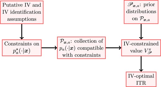
A schematic plot of IV-optimality. Prior distributions imposed on the IV-constrained sets give rise to the IV-constrained value . An IV-optimal ITR maximizes over a policy class Π.
The formulation in (5) can be recovered by carefully choosing the prior distributions. In particular, let and be distributions that witness the partial identification bounds and , respectively:
Then, criterion (5) is recovered by considering the following two-point priors:
where is a point mass at p. As discussed near the end of Section 2.2, setting uniformly equal to recovers the original IV-optimality criterion considered in Pu and Zhang (2021) that minimizes the worst-case risk (4). In fact, under certain regularity conditions, one can show that the reverse is also true: the formulation (7) for a specified collection prior distributions can also be recovered from (5) by a careful choice of λ. In view of such an equivalence, criterion (7) should not be regarded as a generalization of (5). Rather, it is a convenient tool amenable to being generalized to the multiple-stage setting. A proof of this equivalence statement will appear in Section 4.
3 Improving individualized treatment rules with an instrumental variable
Compared to estimating an optimal ITR, a less ambitious goal is to improve upon a baseline ITR , so that the improved ITR is no worse and potentially better than . In this section, we show how to achieve this goal with an IV in the single-stage setup.
The goal of ‘never being worse’ is reminiscent of the min-max risk criterion in (4), and it is natural to consider minimizing the maximum excess risk with respect to the baseline ITR , subject to the IV-informed partial identification constraints. Definition 1 summarizes this strategy.
Risk-based IV-improved ITR
Let denote a baseline ITR, Π a policy class, and an IV-informed partial identification interval of the CATE . A risk-based IV-improved ITR is any solution to the optimization problem below:
When Π consists of all Boolean functions, (9) admits the following explicit solution.
Formula for risk-based IV-improved ITR
Define
Then, is a risk-based IV-improved ITR when Π consists of all Boolean functions.
The ITR in (10) admits an intuitive explanation: it takes action when the partial identification interval is positive (i.e., ), takes action when the interval is negative (i.e., ), and otherwise follows the baseline ITR .
A second criterion closely related to that in Definition 1 maximizes the minimum excess value with respect to , subject to the distributional constraints imposed by the putative IV and its associated identification assumptions.
Value-based IV-improved ITR
Let denote a baseline ITR, Π a policy class, and a collection of IV-constrained sets. A value-based IV-improved ITR is any solution to the following optimization problem:
The above formulation is referred to as distributionally robust optimization in the optimization literature (Delage & Ye, 2010). When the IV-constrained sets are derived from partial identification intervals and Π consists of all Boolean functions, the optimization problem (11) admits the explicit solution below, analogous to the one given in Proposition 1.
Formula for value-based IV-improved ITR
Assume and , the two distributions defined in (8) that witness the partial identification bounds , , are both inside . Define
where and . Then, is a value-based IV-improved policy when Π consists of all Boolean functions.
Propositions 1 and 2 together reveal an interesting duality between worst-case excess risk minimization and worst-case excess value maximization. When the partial identification interval for the CATE is derived directly from the partial identification intervals for the mean conditional potential outcomes, so that and , then the two ITRs defined in (10) and (12) agree, and they simultaneously satisfy the two IV-improvement criteria presented in Definitions 1 and 2. Hence, we will not distinguish between two types of IV-improved ITRs henceforth.
Recall that a similar duality exists in the classical policy estimation problem under the NUCA, but disappears when extended to the partial identification settings. It is thus curious to see such a duality restored in the policy improvement problem.
4 Estimating dynamic treatment regimes with an instrumental variable
4.1 Optimal and SRA-optimal DTRs
We now consider a general K-stage decision-making problem (Murphy, 2003; Schulte et al., 2014). At the first stage , we are given baseline covariates , make a decision , and observe a reward . At stage , let denote treatment decisions from stage 1 up to , and the rewards from stage 1 to . Meanwhile, denote by new covariate information (e.g., time-varying covariates, auxiliary outcomes, etc.) that would arise after stage but before stage k had the participant followed the treatment decisions , and the entire covariate history up to stage k. Given , a data-driven decision is then made and we observe reward . Our goal is to estimate a DTR , such that the expected value of cumulative rewards is maximized if the population were to follow π.
To simplify the notations, the historical information available for making the decision at stage k is denoted by for and for any The information consists of and : is the information available at the previous stage and is the new information generated after decision is made. Let be the conditional law of given a specific realization of the historical information . We define the following action-value function (or Q-function) at stage K:
where we emphasize again that the expectation is taken over the potential outcome distribution . For a policy π, its value function at stage K is then defined as
and depends on π only through .
Next, we define Q-functions and value functions at a generic stage recursively (denote ). In particular, for , we let denote the joint law of the reward and new covariate information observed immediately after decision has been made conditional on . The Q-function of π at stage k is then defined as:
where is a function of and . The corresponding value function of π is taken to be Similar to (13), the expectation is taken over the potential outcome distribution . We interpret the Q-function as the cumulative rewards collected by executing at stage k and follow π from stage and onwards, and the value function the cumulative rewards collected by executing π from stage k and onwards. Therefore, depends on π only via and depends on π only via . For notational simplicity, we interpret quantities whose subscripts do not make sense (e.g., , and ) as ‘null’ quantities and their occurrences in mathematical expressions will be disregarded.
With a slight abuse of notation, we let be a policy class. A DTR is said to be optimal with respect to Π if it maximizes for all fixed (and hence for an arbitrary covariate distribution) over the policy class Π.
Assume for now that Π consists of all DTRs (i.e., each consists of all Boolean functions). A celebrated result from the control theory states that the dynamic programming approach below, also known as backward induction, yields an optimal DTR (Murphy, 2003; Sutton & Barto, 2018):
In other words, satisfies for any and historical information , and is well defined as depends on only through .
The foregoing discussion is based on the potential outcome distributions. Suppose that we have collected i.i.d. data from the law of the random trajectory . Let be the conditional laws of the observed rewards and new covariate information identified from the observed data:
Here, denotes the observed historical information up to stage k. Suppose that we obtain a DTR using the dynamic programming approach described in (15) with in place of . Under a version of the sequential randomization assumptions (Robins, 1998) and with additional assumptions of consistency and positivity, we have from which it follows that the DTR is optimal (Murphy, 2003; Schulte et al., 2014). We will refer to this policy as an SRA-optimal DTR and denote it as .
4.2 Identification with a time-varying instrumental variable
Suppose that, in addition to , we also observe a binary, time-varying instrumental variable at each stage k and write . The time-varying IV is said to be valid if it satisfies the longitudinal generalizations of core IV assumptions including IV relevance: for all k, exclusion restriction: for all k and , and IV unconfoundedness: . The IV unconfoundedness assumption holds by design in sequential randomized trials and is more likely to hold conditional on historical information for IV studies using observational data. The IV unconfoundedness assumption may also be replaced by weaker exchangeability assumptions discussed in Swanson et al. (2018, Section 2).
It is essential to have a time-varying IV (e.g., daily precipitation) rather than a time-independent IV (e.g., genetic variant like the sickle cell trait) in this setting. To illustrate this point, Figure 3 exhibits a causal direct acyclic graph (DAG) for : and are time-varying IVs, and treatment received, and outcomes, and , , and U unmeasured confounders. We omit any observed covariates for clearer presentation. Figure 3 explicitly differentiates between two types of unmeasured confounding in the DAG: and represent unmeasured confounding specific to the first and second stages, and U represents unmeasured confounding shared between both stages. When studying the effect of on , is a valid IV for ; on the contrary, is not a valid IV for , because conditioning on induces association between and U (represented by the dashed line in the DAG), thus violating the IV unconfoundedness assumption (Hernán et al., 2004), and not conditioning on (i.e., marginalizing over ) violates the exclusion restriction assumption; see, e.g., Verma and Pearl (2022).
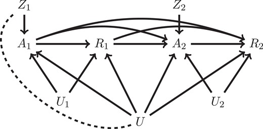
Direct acyclic graph (DAG) when with time-varying IVs. (and ) represents stage (and stage ) unmeasured confounding, and U shared unmeasured confounding. is an IV for and an IV for . is not a valid IV for because conditioning on induces association between and U, and not conditioning on violates exclusion restriction.
Point identification of ’s effect on conditional on historical information is possible under some version of homogeneity or no-interaction assumption. Michael et al. (2020, Section 3) describe sufficient conditions for point identification under a latent variable formulation of an IV model. Their conditions extend those in Wang and Tchetgen Tchetgen (2018) from static to longitudinal settings and generalize the ‘additive unmeasured confounder’ assumption studied in Liao et al. (2021). Michael et al.’s (2020) proposed point identification assumptions essentially entail further restriction that cannot have an additive interaction with any component of unmeasured confounding in affecting the actual treatment received. For instance, in Figure 3, cannot interact with or U and have an additive effect on conditional on , so that all systematic difference in a person’s compliance type at each stage k is completely accounted for by historical information up to stage k.
In the rest of article, we focus on developing a framework that accommodates both point and partial identification. In the context of estimating an ITR, Zhang and Pu (2020) and Pu and Zhang (2021) discussed some desirable features of a partial identification strategy in IV studies. Partial identification allows an IV-optimal ITR be well defined under minimal IV identification assumptions and amenable to different choices of an IV in empirical studies. Moreover, the quality of the estimated IV-optimal ITR adapts to the quality of the selected IV (Pu & Zhang, 2021, Remarks 5 and 6). These considerations remain relevant in estimating a DTR. In a multiple-stage, IV-assisted decision problem, point identification requires posting no-interaction-type assumptions at each stage k. It is likely that the no-interaction-type assumption is deemed reasonable towards later stages after having collected rich covariate history data, but not at initial stages, further necessitating a comprehensive framework covering both modes of identification.
4.3 IV-optimality for DTRs and dynamic programming under partial identification
Similar to the single-stage setting in Section 2.3, the IV at each stage, along with its associated identification assumptions, imposes distributional constraints on the potential outcome distributions . That is, we can specify, for each action and historical information at stage k, an IV-constrained set that contains the ground truth potential outcome distribution . We treat as a generic set of distributions compatible with the IV and identification assumptions for now; concrete examples will be given when we formally describe estimation procedures in Section 4.5.
Given the IV-constrained set , we impose a prior distribution on it. This notion generalizes the single-stage setting in Section 2.3. We use to denote sampling a distribution from . We will use the shorthand for where there is no ambiguity.
Under these notations, we introduce IV-constrained counterparts of the conventional Q- and value functions defined in (13) and (14).
IV-constrained Q- and value function
For each stage , each action , and each configuration of the historical information , let be a prior distribution on the IV-constrained set . The IV-constrained Q-function and the corresponding value function of a DTR π with respect to the collection of prior distributions at stage K are
respectively. Recursively, at stage , the IV-constrained Q-function and the corresponding value function are
respectively, where is a function of and .
Similar to the conventional Q- and value functions, the IV-constrained Q-function depends on π only through and the IV-constrained value function depends on π only through .
Definition 4 follows from Definition 3 and defines IV-optimality for DTRs.
IV-optimal DTR
A DTR is said to be IV-optimal with respect to the collection of prior distributions and a policy class Π if it satisfies
for every fixed .
Theorem 1 proves that an IV-optimal policy that maximizes the IV-constrained value function for every exists and can be obtained via a modified dynamic programming algorithm when Π consists of all policies.
Dynamic programming for the IV-optimal DTR
Let be recursively defined as follows:
Then, the DTR satisfies
for any stage k and any configuration of the historical information , where the maximization is taken over all DTRs.
Theorem 1 generalizes the classical dynamic programming algorithm under a partial identification scheme. The policy in Theorem 1 is always well-defined as depends on only through .
4.4 An alternative characterization of IV-optimal DTRs
Estimation of an IV-optimal DTR based on Theorem 1 is difficult, as the definitions of the IV-constrained Q- and value functions involve integration over the prior distributions , which may be difficult to specify. Recall that in the single-stage setting, there is an equivalence between the IV-constrained value (7) and the convex combination of the lower and upper bounds of value (5). The convex combination is easier to compute provided that the weights are specified. We now extend this equivalence relationship to the multiple-stage setting to get rid of the intractable integration over prior distributions and facilitate a practical estimation strategy.
We start by defining the worst-case and best-case IV-constrained Q- and value functions as well as their weighted versions as follows.
Worst-case, best-case, and weighted Q- and value functions
Let the prior distributions be specified and be a collection of weighting functions taking values in . The worst-case, best-case, and weighted Q-functions at stage K with respect to and are defined as
The corresponding worst-case, best-case, and weighted value functions, denoted as , , and , respectively, are obtained by setting in the above displays. Recursively, at stage , we define the worst-case, best-case, and weighted Q-functions as
respectively. Again, replacing in the above Q-functions with yields their corresponding value functions , and .
Definition 5 generalizes criterion (5). According to Definition 5, the worst-case and best-case Q-functions and depend on the weighting functions only through for , whereas the corresponding value functions depend on the weighting functions only through for . For notational simplicity, we will add superscript π and subscript in Q-functions at stage K (e.g., we write ), although they have no dependence on π or the weighting functions.
Proposition 3 establishes the equivalence between the weighted Q-functions (resp. value functions) and their IV-constrained counterparts in Definition 3.
Equivalence between weighted and IV-constrained Q- and value functions
The following two statements hold:
Fix any collection of weighting functions . Assume that in Definition 5, the infimums and supremums when defining weighted Q- and value functions are all attained. Then, there exists a collection of prior distributions such that
Reversely, if any collection of prior distributions is fixed, then there exists a collection of weighting functions such that the above display holds true.
Proposition 3 effectively translates the problem of specifying a collection of prior distributions to specifying a collection of weighting functions, thus allowing one to bypass integration over prior distributions. Combine Proposition 3 and Theorem 1 and we have the following alternative characterization of the IV-optimal DTR.
Alternative characterization of the IV-optimal DTR
Under the setting in Part 1 of Proposition 3, if we recursively define as
where the two quantities
depend on only through and are hence well-defined, then satisfies (17) for any stage k and any configuration of the historical information . In particular, is an IV-optimal DTR in the sense of Definition 4 when Π consists of all Boolean functions.
As an alternative to Theorem 1, Corollary 1 gives an analytic and constructive characterization of the IV-optimal DTR.
Figure 4 illustrates the decision process when . At the second stage, given and , an IV-optimal action is made based on comparing two weighted Q-functions and , and we have . Analogously, we have .
Given the knowledge of , we can compute the weighted value function of at the second stage. This allows us to construct a ‘pseudo-outcome’ at the first stage, denoted as . Importantly, depends on , as it is the cumulative rewards if we observe at the first stage, take an immediate action , and then act according to the IV-optimal decision at the second stage.
The partial identification interval for the expected value of , where the expectation is taken over the potential outcome distribution of and , is precisely the worst-case and best-case Q-functions and . We can then compute the weighted Q-function given , from which we can decide . Reading the numbers off Figure 4, we conclude that .
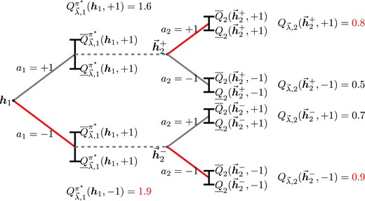
An illustrative example of an IV-optimal DTR when . According to the values of the weighted Q-functions at , we have and . Given , the weighted Q-functions at can be computed, and the IV-optimal action is .
Weighting functions
The specification of weighting functions reveals one’s level of optimism. Fix all future weighting functions . At stage k, if one adopts a worst-case perspective and would like to maximize the worst-case gain at this stage, then it suffices to compare the two worse-case Q-functions at stage k, namely and . This pessimistic action equals the sign of the difference of the two worst-case Q-functions and corresponds to taking (see Figure 5a). Alternatively, if one adopts a best-case perspective at stage k and would like to maximize the best-case gain at this stage, then one compares the two best-case Q-functions, namely and . This optimistic action equals the sign of the difference between the two best-case Q-functions and corresponds to taking (see Figure 5b). Recall that in the single-stage setting, the min-max risk criterion (4) corresponds to maximizing the weighted value (5) with weights set to be . This criterion can be seamlessly generalized to the current multiple-stage setting by setting (see Figure 5c). Other choices of weighting functions can also be made to incorporate domain knowledge and reflect individual-level preference, as suggested by Cui and Tchetgen Tchetgen (2021).
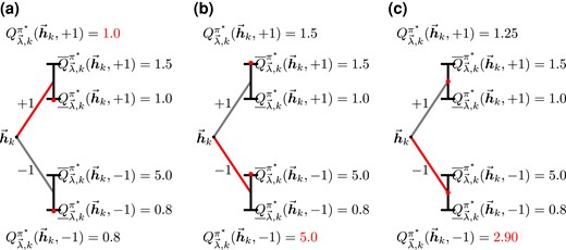
IV-optimal DTR at stage k with different choices of weighting functions. The weighted Q-functions are marked by red dots, and the corresponding IV-optimal action is coloured in red. (a–c) correspond to the worst-case, best-case, and the min-max perspectives, respectively. In each case, the IV-optimal action is . (a) Worst: . (b) Best: . (c) Min-max: .
4.5 Estimating IV-optimal DTRs
According to Corollary 1, it suffices to estimate the weighted Q-functions and hence contrast functions defined in (22) in order to estimate the IV-optimal DTR . We first consider a Q-learning approach to the estimation problem (Schulte et al., 2014; Watkins & Dayan, 1992). As a concrete example, we estimate the worst-case and best-case Q-functions using Manski and Pepper’s ‘minimal-assumptions’ bounds that depend only on core IV assumptions (Manski, 1997; Manski & Pepper, 2000). These core IV assumptions are automatically satisfied, for instance, in a SMART design with noncompliance. In the Online Supplementary Material S5, we review other useful partial identification bounds, including those depending on the monotone instrumental variable assumption, monotone treatment selection assumption (MTS), and monotone treatment response assumption (MTR).
At Stage K, define
Manski-Pepper bounds state that if almost surely, then its conditional mean potential outcome is lower bounded by
and upper bounded by
Hence, we set , , and construct the stage-K weighted Q-function provided values of . In practice, we may estimate all relevant quantities from the observed data by fitting parametric models (e.g., linear models) or flexible machine learning models (e.g., regression trees and random forests) and then invoke the plug-in principle.
Given an estimate of , we can then estimate the contrast function by , and the stage-K IV-optimal DTR can be estimated by according to Corollary 1. Moreover, the weighted value function of at stage K, , can be estimated by .
Now, assume for any stage , the stage-t weighted value function has been estimated by , and that almost surely. At stage k, define the pseudo-outcome . By construction, we have almost surely for . Thus, we can apply Manski-Pepper bounds (or other partial identification bounds) one more time to bound the expected value of . Alternatively, two terms involved in the pseudo-outcome may be bounded separately using some stylized bounds based on firm domain knowledge; see Online Supplementary Material S5 for details. In this way, we obtain an estimate of the weighted Q-function of at stage k; see Online Supplemental Material S4 for detailed expressions. One nuance is that the pseudo-outcome depends on the unknown quantity . At stage k, we have already obtained an estimate of . Thus, the pseudo-outcome can be estimated by .
Finally, the contrast function is estimated by , the stage-k IV-optimal DTR by , and the stage-k weighted value function by . In this way, we recursively estimate all contrast functions and obtain an estimated IV-optimal DTR .
Estimation of the IV-Optimal DTR
| Input: Trajectories and instrument variables |
| , weighting functions , policy class Π, forms of partial identification intervals. |
| Output: Estimated IV-optimal DTR . |
| # Step I: Q-learning |
| Obtain an estimate of using ; |
| Estimate by ; |
| Set and ; |
| fordo |
| For each , construct ; |
| Obtain an estimate of using using ; |
| Estimate by ; |
| Set and |
| end |
| # Step II: Weighted classification |
| for do |
| Solve the weighted classification problem in (24) to obtain ; |
| end |
| return |
In many applications, it may be desirable to obtain parsimonious and interpretable DTRs inside some prespecified function class . To achieve this, we may ‘project’ , the DTR obtained by Q-learning and is thus not necessarily inside Π, onto the function class Π. With some algebra, one readily checks that is a solution to the following weighted classification problem:
This representation illuminates a rich class of strategies to search for a DTR π within a desired, possibly parsimonious function class Π, via sequentially solving the following weighted classification problem:
where we recall that is an estimate of obtained via Q-learning, and is the historical information at stage k in our dataset. This strategy is similar to the proposal in Zhao et al. (2015). Algorithm 1 summarizes the procedure.
4.6 Improving dynamic treatment regimes with an instrumental variable
The IV-optimality framework developed in Sections 4.3–4.5 can be modified to tackle the policy improvement problem under the multiple-stage setup. Let be a baseline DTR to be improved. Some most important baseline DTRs include the standard-of-care DTR (i.e., for any k) and the SRA-optimal DTR defined in Section 4.1. The goal of policy improvement, as discussed in Section 3, is to obtain a DTR such that is no worse and potentially better than .
Similar to the materials in Sections 4.3–4.5, one can leverage additional information encoded in the collection of IV-constrained sets . Briefly speaking, instead of starting from the usual value function, one now starts from the ‘relative’ value function, which characterizes the excess value collected by a certain policy compared to the baseline policy . One can then define the notion of IV-improved DTRs using similar constructions as those appeared in Sections 4.3–4.5. We refer the readers to Online Supplemental Material S1 for a detailed exposition.
5 Theoretical properties
In this section, we prove nonasymptotic bounds on the deviance between the estimated IV-optimal DTR to its population counterpart. The theoretical guarantees for IV-improved DTR are deferred to Online Supplementary Material S1.2.
We need several standard assumptions, which we detail below. First of all, we need a proper control on the complexity of the policy class . Note that any is a Boolean function that sends a specific configuration of the historical information to a binary decision . Let be the collection of all possible s. A canonical measure of complexity of Boolean functions is the Vapnik–Chervonenkis (VC) dimension (Vapnik & Chervonenkis, 1968). The VC dimension of , denoted as , is the largest positive integer d such that there exists a set of d points shattered by , in the sense that for any binary vector , there exists such that for . If no such d exists, then .
In practice, a DTR is most useful when it is parsimonious. For this reason, the class of linear decision rules and the class of decision trees with a fixed depth are popular in various application fields (Speth et al., 2020; Tao et al., 2018). It is well known that when the domain is a subset of , the VC dimension of the class of linear decision rules is at most [see, e.g., Example 4.21 of Wainwright (2019)] and the VC dimension of the class of decision tree with L leaves is (Leboeuf et al., 2020).
Note that a DTR , along with the distributions , induces a probability distribution on , the set of stage-k historical information. Let denote the set of all such probability distributions when we vary and for . An element in will be denoted as , and the law of will be denoted as . The next assumption concerns how much information on can be generalized to the information on a specific .
Bounded concentration coefficients
Suppose there exist positive constants such that
Assumption 1 is often made in the reinforcement learning literature (see, e.g., Chen & Jiang, 2019; Munos, 2003; Szepesvári & Munos, 2005) and is closely related to the ‘overlap’ assumption in causal inference. A sufficient condition for the above assumption to hold is that the probability of seeing any historical information (according to the observed data distribution or any distribution in ) is strictly bounded away from 0 and 1.
Recall that our proposed algorithm for estimating an IV-optimal DTR is a two-step procedure, where in Step I, the contrast functions are estimated via Q-learning, and in Step II, a parsimonious DTR is obtained via weighted classification. As mentioned in Section 4.5, in the first step, there is a lot of flexibility in choosing the specific models and algorithms for estimating the contrast functions, and a fine-grained understanding of this step would require a case-by-case analysis. In order not to over-complicate the discussion, we assume the existence of a ‘contrast estimation oracle’.
Existence of the contrast estimation oracle
Suppose in Q-learning, we use an algorithm that takes n i.i.d. samples and outputs that satisfy
for any , where the probability is taken over the randomness in the n samples and the expectation is taken over the randomness in a fresh trajectory .
Assumption 2 is usually a relatively mild assumption. The ground truth contrast functions are superimpositions of several conditional expectations of the observed data distribution, and it is reasonable to assume that they can be estimated at a vanishing rate as the sample size tends to infinity. While this assumption simplifies the analysis by bypassing the case-by-case analyses of Q-learning, the analysis of the weighted classification remains nontrivial.
To proceed further, we adopt a form of sample splitting procedure called cross-fitting (Athey & Wager, 2020; Chernozhukov et al., 2018). Specifically, we split the n samples into m equally-sized batches: , where and (i.e., of constant order). Each batch has size . For each , let be the index of its batch, so that . For the ith sample, we apply the contrast estimation oracle in Assumption 2 on the out-of-batch samples to obtain either an estimate of . We then solve the following optimization problem:
We emphasize that cross-fitting is mostly for theoretical convenience. The performance of our algorithm with and without cross-fitting is similar.
In practice, given a limited computational budget, we may only solve the optimization problem (26) up to a certain precision. Our analysis will be conducted for the approximate minimizer that satisfies
respectively, where is the optimization error when solving (26).
To quantify the loss of information from restriction to the policy class Π, we define
Note that according to Corollaries 1, when is the set of all Boolean functions, we have . Otherwise, the difference between and measures the approximation error when we restrict ourselves to instead of the set of all Boolean functions in the policy estimation (resp. policy improvement) problem.
We are now ready to present the main result of this section.
Performance of the estimated IV-optimal DTR
Let Assumptions 1 and 2 hold. Fix any . Let the optimization error be . Let the approximation error be
where denotes the DTR that acts according to at stage k and follows from stage to K. Finally, define the generalization error
Then, there exists an absolute constant such that with probability , we have
In the above display, the expectations are taken over a fresh sample of the observed first stage covariates .
Theorem 2 shows that the weighted value function of at the first stage converges to that of the IV-optimal DTR up to three sources of errors: the optimization error that stems from approximately solving the weighted classification problem, the approximation error that results from the restriction to a parsimonious policy class Π, and a vanishing generalization error. We defer the proof to Online Supplemental Material S3.
6 Simulation studies
6.1 Comparing IV and non-IV approaches
We considered a data-generating process with two time-independent covariates , . At stage one, there exist an unmeasured confounder , an instrumental variable , a treatment assignment that is Rademacher with probability , and a reward that is Bernoulli with probability , where . According to this data-generating process, treatment has no causal effect on for those with but a modest effect for those with . The unmeasured confounder represents some unmeasured disease severity, so that patients with are more likely to receive treatment and have a smaller reward . This mimics the NICU application where sicker mothers are more likely to deliver in high-level NICUs and these sicker mothers and their newborns are at higher risk. Because of the unmeasured confounder , a naive non-IV analysis based on the observed data underestimates the treatment effect of on . At the second stage, there exist a second unmeasured confounder , a second instrumental variable , a second treatment assignment that is Rademacher with probability , and a second reward that is Bernoulli with probability . Similar to , represents unmeasured risk factors and a naive, non-IV analysis ignoring underestimates the treatment effect of on . Parameters C in the above data-generating process controls the strength of IV-treatment association and controls the level of unmeasured confounding. Both parameters C and will be varied later.
An ‘SRA-optimal’ DTR does not leverage the IV data and is based solely on the observed data and falsely assumes the SRA. To estimate , we estimated the CATE using a robust stabilized augmented inverse probability weighting estimator (SAIPW) and then applied a weighted classification routine. This is known as C-learning in the literature (Zhang & Zhang, 2018), and it can also be viewed as a variant of the backward outcome weighted learning procedure (Zhao et al., 2015). We then estimated the IV-optimal DTR corresponding to for . When constructing the IV-optimal DTRs, we used ‘minimal-assumptions’ bounds (Balke-Pearl bounds for a binary outcome and Manski-Pepper bounds otherwise). All classification problems involved in estimating and were implemented using a classification tree with a maximum depth of 2, which is meant to replicate the real data application where parsimonious rules are more useful and may deliver most insight (Laber & Zhao, 2015; Speth et al., 2020). Finally, we evaluated each estimated regime by generating fresh samples of and integrating out the unmeasured confounders and .
Figure 6 summarizes the cumulative distribution functions of the value of estimated SRA-optimal policy and IV-optimal policy when and for assorted training sample sizes n and levels of confounding . It is transparent that the IV-based approach has superior performance compared to the non-IV approach in all of these cases; moreover, the improvement becomes more conspicuous as the sample size increases. Table 1 further puts the percentage of improvement in the context of maximal possible improvement (comparing an optimal policy to a baseline policy that treats no one). For instance, when and , the IV-based DTR attained a median of of maximal possible improvement, while the non-IV approach only attained a median of of maximal possible improvement. What explained the performance gap between IV and non-IV methods? The SAIPW estimates obtained from a naive non-IV approach tended to underestimate the treatment effect and indicate a spurious, negative treatment effect at either stage as a result of omitting the unmeasured confounders. Therefore, the estimated often recommended withholding the treatment even when the treatment was in fact beneficial. On the other hand, the IV-based interval estimates of the CATEs more faithfully tracked the genuine treatment effect. This difference in estimating the CATE then translated into the performance gap between IV and non-IV DTRs. In Online Supplementary Material S6, we further report simulation results corresponding to different levels of IV-treatment association as controlled by the parameter C. We found two consistent trends. First, achieved better performance when the IV-treatment association increases (that is, when C grows holding fixed). Second, IV-optimal DTR consistently outperformed in these simulation settings though the degree of improvement depends on the specifics of the data-generating processes.
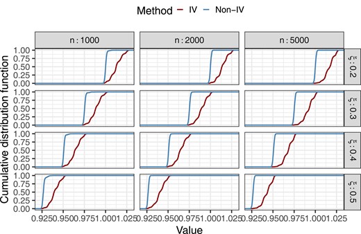
Cumulative distribution functions of the value of the estimated SRA-optimal policy and IV-optimal policy (min-max) for various n and values and .
Performance of IV and non-IV approaches for various training sample sizes n and levels of unmeasured confounding when
| Non-IV method: | IV method: | |||||||
|---|---|---|---|---|---|---|---|---|
| % Improvement | % Correct | % Improvement | % Correct | |||||
| Median | IQR | Stage I | Stage II | Median | IQR | Stage I | Stage II | |
| n = 1000 | ||||||||
| 0.2 | 12.4 | [10.2, 14.9] | 0.0 | 0.9 | 51.0 | [35.9, 68.3] | 45.0 | 58.9 |
| 0.3 | 14.5 | [11.8, 17.2] | 0.1 | 1.4 | 58.9 | [45.9, 76.1] | 47.6 | 61.7 |
| 0.4 | 12.8 | [10.3, 15.3] | 0.1 | 1.8 | 58.3 | [46.4, 76.9] | 51.0 | 62.4 |
| 0.5 | 13.6 | [10.3, 16.5] | 0.2 | 3.1 | 61.5 | [50.4, 81.6] | 51.2 | 63.5 |
| n = 2000 | ||||||||
| 0.2 | 12.3 | [10.1, 14.6] | 0.0 | 0.0 | 54.2 | [45.5, 70.1] | 49.0 | 64.4 |
| 0.3 | 14.6 | [11.8, 17.2] | 0.0 | 0.1 | 62.3 | [51.2, 79.0] | 51.1 | 67.0 |
| 0.4 | 12.6 | [10.1, 15.0] | 0.0 | 0.1 | 59.8 | [49.9, 76.5] | 50.6 | 67.2 |
| 0.5 | 13.1 | [10.3, 16.1] | 0.0 | 0.1 | 64.6 | [53.5, 82.5] | 53.5 | 66.7 |
| n = 5000 | ||||||||
| 0.2 | 12.4 | [10.1, 14.6] | 0.0 | 0.0 | 65.7 | [50.1, 74.5] | 57.0 | 74.4 |
| 0.3 | 14.3 | [11.6, 17.1] | 0.0 | 0.0 | 74.0 | [55.2, 83.3] | 60.0 | 73.7 |
| 0.4 | 12.7 | [10.0, 15.5] | 0.0 | 0.0 | 73.4 | [55.8, 86.2] | 62.8 | 76.8 |
| 0.5 | 13.4 | [10.4, 16.2] | 0.0 | 0.0 | 77.7 | [58.1, 92.6] | 60.1 | 77.9 |
Note. The metric % Improvement is defined as the improvement in the value as a fraction of the maximal possible improvement (comparing an optimal policy to a baseline policy that treats no one). The metric % Correct at Stage II is defined as the percentage of subjects with who are assigned by the estimated DTR. The metric % Correct at Stage I is defined as the percentage of subjects with who are assigned by the estimated DTR.
6.2 Additional simulation results
In Online Supplementary Material S7, we verified that IV-improved DTRs had superior performance compared to their corresponding baseline DTRs, including an SRA-optimal DTR. In Online Supplementary Material S8.1, we discussed the primary difference between two IV-based approaches: a Wald-estimator-based, point-identification approach and the more generic, partial identification approach. Without additional identification assumptions, a conditional Wald estimator identifies the conditional local average treatment effect, which is the average treatment effect among a latent subgroup known as compliers conditional on observed covariates. When there is treatment heterogeneity among different latent subgroups, e.g., when the treatment effect among compliers and that among the rest of the population are different, then a Wald-estimator-based approach may mistakenly assign study participants to treatment even when they are hurt by the treatment assignment on average conditional on covariate history. Simulation results that confirm this can be found in Online Supplementary Material S8.2 and S8.3.
7 Application
We considered a total of mothers who delivered exactly two births during 1995 and 2009 in the Commonwealth of Pennsylvania and relocated at their second deliveries so that their ‘excess-travel-time’ IVs at two deliveries were different. We followed the study design in Baiocchi et al. (2010) and Lorch et al. (2012) and controlled for covariates that measured mothers’ neighbourhood circumstances including poverty rate, median income, etc., mothers’ demographic information including race (white or not), age, years of education, etc., and variables related to delivery including gestational age in weeks and length of prenatal care in months, and eight congenital diseases; see Online Supplemental Material S9 for details. The ‘excess-travel-time’ IVs in both stages were then dichotomized: 1 if above the median and 0 otherwise. Mothers’ treatment choice and their babies’ mortality status at the first delivery were included as covariates for studying the second delivery. We used the multiple imputation by chained equations method (Buuren & Groothuis-Oudshoorn, 2010) implemented in the R package MICE to impute missing covariate data and repeated the analysis on five imputed datasets.
We assume that high-level NICUs do no harm compared to low-level NICUs; therefore, all partial identification intervals in this application were estimated under the MTR assumption (Manski, 2003, Chp. 8). We considered estimating an IV-optimal DTR minimizing the maximum risk at each delivery (see Section 4.4) and explored the trade-off between minimizing the maximum risk and the cost/capacity constraint by adding a generic penalty to the value function. We performed weighted classification using a classification tree with maximum depth equal to 3 so that the resulting DTR is interpretable. Figure 7 plots three estimated DTRs corresponding to no penalty attached, a moderate penalty, and a large penalty attached to attending a high-level NICU. When there is no penalty attached, all mothers are assigned to a high-level NICU. As we increase the penalty, fewer mothers (albeit mothers who benefit most from attending a high-level NICU) are assigned to a high-level NICU. For instance, Figure 7b corresponds to sending mothers to a high-level NICU at their first deliveries and at their second deliveries. Mothers assigned to a high-level NICU according to this DTR either belong to racial and ethnic minority groups or are older and have premature gestational age. Similarly, Figure 7c plots a regime where less than of mothers are assigned to a high-level NICU. Mothers who are assigned to a high-level NICU according to this DTR belong to racial and ethnicity minority groups and have premature births. Our analysis here seems to suggest that, in general, race and ethnicity, mother’s age, and gestational age are the most promising effect modifiers. Gestational age has long been hypothesized as an effect modifier; see Lorch et al. (2012), Yang et al. (2014), and Michael et al. (2020); more recently, Yannekis et al. (2020) found a differential effect between different races and ethnic groups. On the other hand, mother’s age as an effect modifier appears to be a new discovery that is worth looking into. Overall, our method both complemented previous published results and generated new insights.
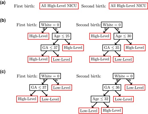
Estimated IV-optimal DTRs using the NICU data. GA is gestational age. (a) No penalty for attending a high-level NICU. All mothers are assigned to high-level NICUs. (b) Moderate penalty for attending a high-level NICU. and of all mothers are assigned to high-level NICUs for their first and second deliveries, respectively. (c) Large penalty for attending a high-level NICU. and of all mothers are assigned to high-level NICUs for their first and second deliveries, respectively.
8 Discussion
We systematically studied the problem of estimating a DTR from retrospective observational data using a time-varying instrumental variable. We formulated the problem under a generic partial identification framework, derived a counterpart of the classical Q-learning and Bellman equation under partial identification and used it as the basis for generalizing a notion of IV-optimality to the DTRs. One important variant of the developed framework is a strategy to improve upon a baseline DTR. As demonstrated via extensive simulations, IV-improved DTRs indeed have favourable performance compared to the baseline DTRs, including baseline DTRs that are optimal under the NUCA.
With the increasing availability of administrative databases that keep track of clinical data, it is tempting to estimate some useful, real-world-evidence-based DTRs from such retrospective data. To make any causal/treatment effect statements from non-RCT data, an instrumental variable analysis is often better received by clinicians. Fortunately, many reasonably good instrumental variables are available, e.g., daily precipitation, geographic distances, service providers’ preference, etc. Many of these IVs are intrinsically time-varying and could be leveraged to estimate a DTR using the framework proposed in this article. In practice, to deliver the most useful policy intervention, it is important to take into account various practical constraints, e.g., those arising from limited facility capacity or increased cost. Our framework can be readily extended to incorporating various constraints.
To make the theoretical analyses versatile, we have assumed Assumptions 1 and 2 as well as the finiteness of VC dimension of policy classes in the current analysis. An alternative route that could potentially yield sharper bounds would be to assume margin-type conditions so that the Q-function has a separation between the optimal and nonoptimal treatments. See, e.g., Qian and Murphy (2011) for applying this strategy to the single-stage setting, and Luedtke and Van Der Laan (2016) and Shi et al. (2020) for extending this strategy to a multiple-stage, non-IV setting.
Acknowledgments
The authors would like to thank Dr. Zongming Ma, Dr. Dylan S. Small, three reviewers and editors for constructive feedback and comments. The authors would like to acknowledge Dr. Scott A. Lorch for the use of the data from the NICU study.
Data availability
The participants of this study did not give written consent for their data to be shared publicly, so due to the sensitive nature of the research supporting data is not available. The authors received no financial support for the research, authorship, and publication of this article.
Supplementary material
Supplementary material are available at Journal of the Royal Statistical Society: Series B online.
References
Author notes
Conflict of interest None declared.
