Causal inference on distribution functions

Lin, Zhenhua; Kong, Dehan; Wang, Linbo

doi:10.1093/jrsssb/qkad008

Abstract

Understanding causal relationships is one of the most important goals of modern science. So far, the causal inference literature has focused almost exclusively on outcomes coming from the Euclidean space $R^{p}$ ⁠. However, it is increasingly common that complex datasets are best summarized as data points in nonlinear spaces. In this paper, we present a novel framework of causal effects for outcomes from the Wasserstein space of cumulative distribution functions, which in contrast to the Euclidean space, is nonlinear. We develop doubly robust estimators and associated asymptotic theory for these causal effects. As an illustration, we use our framework to quantify the causal effect of marriage on physical activity patterns using wearable device data collected through the National Health and Nutrition Examination Survey.

double robustness, Wasserstein space, wearable device

1 Introduction

Causal inference has received increasing attention in contemporary data analysis. So far, researchers in causal inference have engaged almost exclusively in studying causal effects on objects from a linear space, most commonly the Euclidean space $R^{p} .$ On the other hand, in many modern applications, the observed data either naturally emerge or may be summarized as distribution functions. Often in these applications, the interest lies in the causal effect on the distributions themselves, rather than a summary measure such as the mean or the quantiles. Here, we detail an example from the study of physical activities; see the Supplementary Material for additional examples on cellular differentiation and metagenomics.

Physical activities

Example 1

Behavioural scientists are often interested in evaluating the effects of potential risk factors, such as marriage, on physical activity patterns (e.g., King et al., 1998). The physical activity patterns are often recorded over a certain monitoring period. For example, in the National Health and Nutrition Examination Survey 2005–2006, physical activity intensity, ranging from 0 to 32,767 counts per minute, was recorded consecutively for 7 days by a wearable device for subjects at least 6 years old. The trajectory of activity intensity is not directly comparable across different subjects as different individuals might have different circadian rhythms. Instead, the distribution of activity intensity is invariant to circadian rhythms and hence can be compared between groups of individuals (Chang & McKeague, 2020).

On the surface, since the distribution functions belong to L², a linear space endowed with a Euclidean distance, one may directly extend the classical potential outcome framework (Neyman, 1923; Rubin, 1974) in causal inference using Euclidean averages. For example, the mean potential distribution functions may be defined as the expectation of the random potential distribution function, and the causal contrast among different interventions may be defined as the Euclidean distance among the mean potential distribution functions. However, there has been a growing recognition among the statistics and data science community that in many applications, the structure of data summarized by distribution functions may be best captured by the use of nonEuclidean distances (e.g., Arjovsky et al., 2017; Bernton et al., 2019; Courty et al., 2016; del Barrio et al., 1999; Ho et al., 2017; Panaretos & Zemel, 2019; Verdinelli and Wasserman, 2019). One of the most common choices of distance is the so-called Wasserstein distance based on the geometry of optimal transport. When equipped with such a distance, the space of probability measures on a real interval $I$ is referred to as the Wasserstein space, and the average of distribution functions under the Wasserstein distance is known as the Wasserstein barycentre of these distributions.

Significant advances have been made by the emerging field of statistical optimal transport studying the Wasserstein space. For instance, Agueh and Carlier (2011), Bigot et al. (2012), and Kim and Pass (2017) introduced the notion of Wasserstein barycentre of a random distribution and studied its existence, uniqueness, and characteristics. The concept of Wasserstein barycentre, defined in (6), is a generalization of the mean of random variables/vectors to random distributions. Moreover, Bigot et al. (2017) generalized the technique of principal component analysis to data sampled from a Wasserstein space, while Petersen and Müller (2016) and Chen et al. (2021) focused on regression models for such data. Recently, Zhang et al. (2020) and Zhu and Müller (2021) investigated distribution-valued time series and generalized the concept of autoregressive models to Wasserstein spaces, while Zhou et al. (2021) developed a framework for canonical correlation analysis of random distributions. For more related works on statistical data analysis in a Wasserstein space, we refer readers to the survey paper by Bigot (2020) and references therein.

The Wasserstein barycentre and distance have several features that make them particularly appealing for defining causal effects on distribution functions. First, the Wasserstein barycentre reduces to the usual Euclidean mean in the degenerate case where the distribution functions take point mass at real values. Specifically, if δ_t denotes the Dirac delta function with point mass at t, then the Wasserstein barycentre of $δ_{t_{i}}, i = 1, \dots, n$ is $δ_{\bar{t}},$ with $\bar{t} = \sum_{i = 1}^{n} t_{i} / n .$ In contrast, the Euclidean average, defined as the average of the cumulative distribution functions of $δ_{t_{1}}, \dots, δ_{t_{n}}$ ⁠, corresponds to a uniform distribution on t_i, …, t_n. Consequently, in the degenerate case where the random distribution function takes point mass at a random real value, their expectation does not correspond to the point mass function at the expectation of the random real value.

Second, compared with the Euclidean distance and other distances such as the Hellinger distance, the Wasserstein barycentre performs exceptionally well in capturing the structure of random distributions (e.g., Cuturi & Doucet, 2014). In Figure 1, we provide a graphical illustration. The distributions in Figure 1a are unimodal distributions; typical distributions of this kind are adult age-at-death distributions (Chen et al., 2021). One can see from Figure 1b and c that the Wasserstein barycentre preserves unimodality while the Euclidean average does not.

Figure 1.

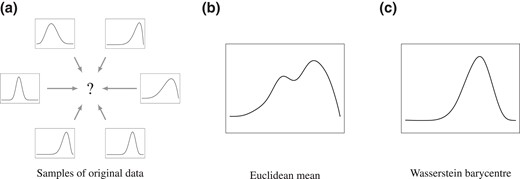
Comparison of Wasserstein barycentre vs. Euclidean average for capturing structural information in random distributions. The barycentre and Euclidean average are based on six unimodal distributions. The Euclidean average has two modes while the Wasserstein barycentre preserves unimodality.

Open in new tab Download slide

Third, the Wasserstein distance has an intuitive interpretation of the amount of ‘work’ required to transform one distribution to another (Sommerfeld & Munk, 2018). Moreover, it comes with a map that shows how to move from one random object to another, and allows one to create a path of distributions that interpolates between Wasserstein barycentres, while preserving the structural information in the random objects. This is particularly useful when comparing two Wasserstein barycentres each representing potential distribution functions under a particular intervention, as it not only contains information on how much they differ, but also on how one of these barycentres can be moved to the other; see Interpretation 2 in Section 3 for more details. In fact, as the path implied by the Wasserstein distance to move distributions involves the ‘least effort’, it is the natural path taken by biological systems to move from one state to another (e.g., Schiebinger et al., 2019).

Lastly, in the Wasserstein space of distributions on an interval of the real line, which is the focus of this paper, the optimal way to transfer one distribution to another is to move between their corresponding quantiles. In this case, the causal effect map defined using optimal transport (see Definition 1) can be directly interpreted as the difference in quantiles of the Wasserstein barycentres of different potential outcome distributions; see Interpretation 1 in Section 3 for more details.

For these advantages and motivated by the applications in Example 1 and Examples S1, S2 in the Supplementary Material, we propose to define causal effects for distribution functions using the optimal transport between the Wasserstein barycentres of different potential outcome distributions. Our definitions of causal effect, called the average causal effect map, can be identified under straightforward generalizations of standard assumptions in the causal inference literature. We develop doubly robust and cross-fitting procedures for estimating the average causal effect map, and establish asymptotic properties for these estimators. In contrast to the setting for the classical doubly robust estimators (Chernozhukov et al., 2018; Robins et al., 1994), typically even for a fixed unit, the outcome may not be fully observed and needs to be estimated from data. For instance, in our real data application, the data consists of empirical distribution functions of physical activity patterns for individuals rather than their underlying distribution functions. To establish the asymptotic properties with distribution-valued outcomes, our analyses rely on several geometric properties of the Wasserstein space, most notably the isometry between the Wasserstein space and the space of quantile functions. To the best of our knowledge, this is the first systematic study on causal inference for distribution-valued outcomes.

The rest of the paper is structured as follows. In Section 2, we present background on causal inference and Wasserstein space. In Section 3, we introduce the notion of average causal effect map for outcomes from a Wasserstein space, and develop identifiability results and doubly robust estimators for the average causal effect map. We then study their asymptotic properties in Section 4. We provide numerical studies in Section 5 and a real data illustration in Section 6. We end with a brief discussion in Section 7.

2 Background

2.1 The potential outcomes framework

We shall define causal effects using the potential outcomes framework. Suppose that the treatment is A ∈ {0, 1}, with 0 and 1 being the labels for control and active treatments, respectively. We use X to denote baseline covariates taking values in $R^{d}$ ⁠. For each level of treatment a, we assume there exists a potential outcome Y(a), representing the outcome had the subject, possibly contrary to the fact, been given treatment a. Here, Y(a) is a random object that resides in a possibly nonlinear space. We make the stable unit treatment value assumption (SUTVA, Rubin, 1980) so that the potential outcomes for any unit do not vary with the treatments assigned to other units, and, for each unit, there are no different versions of treatments that lead to different potential outcomes. Under this assumption, the observed outcome Y = Y(A), where Y(A) = Y(1) if A = 1 and Y(A) = Y(0) if A = 0. We assume we observe n independent samples from an infinite super-population of (A, X, Y), denoted by (A_i, X_i, Y_i), i = 1, …, n.

When Y(a) resides in $R$ ⁠, the causal effect is commonly defined as the contrast between a summary measure of the potential outcome distributions. For example, the average causal effect is defined as the difference between the means of the potential outcome distributions:

ACE = E {Y (1)} - E {Y (0)};

(1)

the quantile treatment effect is defined as the difference between the quantiles of the potential outcome distributions

QTE (α) = F_{Y (1)}^{- 1} (α) - F_{Y (0)}^{- 1} (α), α \in [0, 1],

(2)

where F_Z(z) = P(Z ≤ z) is the cumulative distribution function (CDF) of the random variable Z, and

F_{Z}^{- 1} (α) = inf {z : F_{Z} (z) \geq α}

(3)

is the corresponding quantile function. Causal effects defined in this manner can be interpreted on the population level, as they concern contrasts between potential outcomes in two hypothetical populations. These population-level interpretations concern the effect of introducing a particular treatment to a population and are most relevant to policy makers.

There is, however, a subtle but important distinction between the individual-level interpretations of ACE and QTE(α). Let CE_i = Y_i(1) − Y_i(0) be the individual causal effect for unit i. Individual causal effects provide useful information for individualized treatment decision-making and are most relevant to individual subjects. Since $ACE = E (C E_{i})$ ⁠, it can be interpreted as averages of individual causal effects; here the expectation is taken over units in the super-population. The individual-level interpretation of ACE extends to the conditional average treatment effect, $CACE (L) = E {Y (1) | L} - E {Y (0) | L},$ where L is a subset of observed baseline covariates. In contrast, generally, QTE(α) cannot be interpreted as the α−quantile of individual causal effects. This distinction connects to desideratum (d) in Section 3.1.

2.2 Causal effect identification and estimation

The following assumptions are standard in the causal inference literature (e.g., Hernán & Robins, 2020; Rosenbaum & Rubin, 1983).

Ignorability

Assumption 1

A⫫Y(a) | X, a = 0, 1.

Positivity

Assumption 2

The propensity score π(X) := P(A = 1 | X) is bounded away from 0: There exists $ϵ > 0$ ⁠, such that $ϵ < π (X) < 1 - ϵ, a . e .$

Under Assumptions 1 and 2, when Y(a) resides in $R$ ⁠, the mean potential outcome is given by

μ_{a} : = E [Y (a)] = E_{X} {E [Y | A = a, X]} = E {\frac{I (A = a) Y}{P (A = a | X)}} .

(4)

Similarly, the potential outcome distributions F_Y(a)(y) can be identified by replacing Y in the last term of equation (4) with I(Y ≤ y). Based on (4), the average causal effect can be identified as $ACE = E {Y (1)} - E {Y (0)}$ ⁠, and the quantile treatment effect can be identified as $QTE (α) = F_{Y (1)}^{- 1} (α) - F_{Y (0)}^{- 1} (α)$ ⁠.

Given the identification formula (4), one may use plug-in estimators to estimate the mean potential outcomes. Let $m_{a} (X) = E (Y | A = a, X)$ and f(A | X) = Aπ(X) + (1 − A)(1 − π(X)). Also denote ${\hat{m}}_{a} (X), \hat{π} (X), \hat{f} (A | X)$ as estimates of their corresponding population quantities obtained using standard parametric or nonparametric/machine-learning techniques. Some leading estimators of μ_a include the outcome regression estimator ${\hat{μ}}_{a}^{O R} = P_{n} {\hat{m}}_{a} (X)$ ⁠, the inverse probability weighting (IPW) estimator ${\hat{μ}}_{a}^{I P W} = P_{n} I (A = a) Y / \hat{f} (A | X),$ and the so-called doubly robust estimator ${\hat{μ}}_{a}^{D R} = {\hat{μ}}_{a}^{O R} + P_{n} [(I (A = a) / \hat{f} (A | X)) {Y - {\hat{m}}_{a} (X)}]$ ⁠; here $P_{n}$ refers to the empirical average operator: $P_{n} (O) = (1 / n) \sum_{i = 1}^{n} O_{i}$ ⁠.

2.3 Wasserstein space

Let $I$ be an interval of $R$ ⁠, V₁ and V₂ be random variables taking values in $I$ with finite second moments, and λ₁, λ₂ be their (cumulative) distribution functions, respectively. To define the Wasserstein distance between λ₁ and λ₂, we let Λ(λ₁, λ₂) denote all joint distributions λ₁₂ of (V₁, V₂) that have marginal distributions λ₁ and λ₂. The (2-)Wasserstein distance between λ₁ and λ₂ is defined as

W_{2} (λ_{1}, λ_{2}) = {(inf_{λ_{12} \in Λ (λ_{1}, λ_{2})} \int_{I \times I} (s - t)^{2} d λ_{12} (s, t))}^{1 / 2} .

(5)

The Wasserstein space of order 2 on $I$ is then defined as the space of distribution functions on $I$ with finite second moments

W_{2} (I) = {λ is a distribution function on I : \int_{I} t^{2} d λ (t) < \infty}

endowed with the 2-Wasserstein distance.

The Wasserstein distance can be motivated by the problem of optimal transport. Consider a pile of mass on space $I$ with a distribution λ₁. We wish to transport the mass in such a way that the new mass distribution is λ₂. Assume also that the cost of transporting a unit mass from point s to point t is (s − t)². A transport plan to move λ₁ to λ₂ can be described by the function λ₁₂ such that dλ₁₂(s, t) denotes the amount of mass to move from s to t. Since the amount of mass to be moved out of s must match dλ₁(s), and the amount of mass to be moved into t must match dλ₂(t), we have $\int_{t \in I} d λ_{12} (s, t) = d λ_{1} (s), \int_{s \in I} d λ_{12} (s, t) = d λ_{2} (t)$ ⁠. In other words, λ₁₂ ∈ Λ(λ₁, λ₂). The Wasserstein distance then corresponds to the minimum effort that is required in order to transport the mass of λ₁ to produce the mass distribution of λ₂. The minimizer $λ_{12}^{*}$ to the problem in (5) always exists (Santambrogio, 2015, Theorems 1.7 and 1.22) and is known as the optimal transport plan.

If λ₁ is continuous, then there exists a unique function $T (\cdot) : I \to I$ such that $d λ_{12}^{*} (s, T (s)) = d λ_{1} (s)$ (Santambrogio, 2015, Theorems 1.7 & 1.22). Intuitively, in this case, the optimal transport plan moves all the mass at s to T(s). The function T(·) is known as the optimal transport map. Let λ⁻¹ be the quantile function of the distribution λ. It can be shown that (Ambrosio et al., 2005, Theorem 6.0.2) the optimal transport map $T (s) = λ_{2}^{- 1} (λ_{1} (s))$ ⁠, so that it moves mass between corresponding quantiles of λ₁ and λ₂. The following proposition, summarizing the above discussion, shows that given a fixed continuous distribution λ₁, the distribution λ₂ can be defined via the optimal transport map from λ₁ to λ₂. The proof of Proposition 1 is straightforward and hence omitted.

Proposition 1

Given a continuous distribution function λ₁, there is a one-to-one correspondence between a distribution function λ₂ and the optimal transport map from λ₁ to λ₂.

Based on the notion of Wasserstein distance W₂, we can define the mean of a set of distributions λ₁, …, λ_n in the Wasserstein space by the so-called Wasserstein barycentre $\bar{λ}$ ⁠, defined as the distribution λ that minimizes $(1 / n) \sum_{i = 1}^{n} W_{2}^{2} (λ_{i}, λ)$ ⁠. In Lemma S2 in the Supplementary Material, it is shown that ${\bar{λ}}^{- 1} = (1 / n) \sum_{i = 1}^{n} λ_{i}^{- 1},$ so that the quantile function corresponding to the Wasserstein barycentre equals the (Euclidean) averages of the individual quantile functions. The mean of distributions can also be defined in various other ways, such as the mean under the Euclidean distance $(1 / n) \sum_{i = 1}^{n} λ_{i}$ ⁠. Compared with alternative centre measures, the Wasserstein barycentre typically provides a better summary that captures the structure of the random objects represented by distribution functions, such as shapes, curves, and images; see for example, Figure 1 and Cuturi and Doucet (2014, Figure 1) for illustrations.

3 Causal inference on distribution functions

3.1 Definition of causal effects

We now introduce a definition of average causal effect for outcomes taking value in the Wasserstein space $W_{2} (I)$ ⁠. In parallel to the definition of causal effects introduced in Section 2.1, we first define the mean potential outcomes. As both Y_i(1) and Y_i(0) take value in the Wasserstein space, we define their means using their Wasserstein barycentres:

μ_{a} = E \circ Y (a) ≡ \underset{υ \in W_{2} I}{\arg \min} E {W_{2}^{2} (Y (a), ν)}, a = 0, 1.

(6)

Intuitively, μ_a is a ‘typical’ potential distribution under treatment A = a. Let δ_t denote the Dirac delta function with point mass at t. Ideally, a causal effect definition in the Wasserstein space should satisfy the following desiderata:

When $E \circ Y (1) = E \circ$ Y(0), the causal effect equals zero;
In the degenerate case where $Y_{i} (a) = δ_{y_{i} (a)}$ ⁠, corresponding to the classical scenario where the outcome resides in $R$ ⁠, the causal effect corresponds to the usual average causal effect ACE defined in (1);
The average causal effect is a contrast between the averages of potential outcomes in two hypothetical populations, Y(1) and Y(0), and thus can be interpreted on the population level;
The average causal effect equals the average of individual causal effects, thus maintaining the individual-level interpretation of the ACE for real-valued outcomes discussed at the end of Section 2.1.

Desideratum (a) is natural, given the causal effect is defined as a comparison between two (hypothetical) populations. Desideratum (b) ensures that the definition is a generalization of the standard definition of the ACE (1) in the Euclidean space. Desiderata (c) and (d) are in place to ensure that the definition can be interpreted at both population and individual levels.

From an optimal transport point of view, it may be tempting to define the causal effect as the Wasserstein distance between μ₁ and μ₀; see Section S2 in the Supplementary Material for more discussions on causal effect defined in this way. Although causal effect defined in this way satisfies desiderata (a)–(c), in general, it fails to satisfy desideratum (d). Instead, we introduce a novel definition of average causal effect, called the causal effect map. In Section 3.2, we shall see that the causal effect map satisfies all the desiderata, and contains richer information than the single summary measure W₂(μ₁, μ₀); in particular, one can compute W₂(μ₁, μ₀) based on the causal effect map.

Definition 1

Let λ be a continuous distribution function. The individual causal effect map of A on Y is defined as

Δ_{i}^{λ} (\cdot) = Y_{i} (1)^{- 1} \circ λ (\cdot) - Y_{i} (0)^{- 1} \circ λ (\cdot),

where we say λ is a reference distribution; for a = 0, 1, Y_i(a)⁻¹ is the quantile function of the distribution Y_i(a) as defined in (3). The (average) causal effect map of A on Y is defined as

Δ_{i}^{λ} (\cdot) = (E \circ Y_{i} (1))^{- 1} \circ λ (\cdot) - (E \circ Y_{i} (0))^{- 1} \circ λ (\cdot) = (μ_{1}^{- 1} - μ_{0}^{- 1}) \circ λ (\cdot) .

A crucial component in Definition 1 is the choice of reference distribution λ, that is allowed to have a domain different from that of Y. In general, a different reference distribution leads to a different interpretation of the causal effect maps. Hence, one should choose the reference distribution based on the desired interpretation. We now illustrate some common choices of λ with their interpretations.

Difference in quantiles

Interpretation 1

If the reference distribution λ is the uniform distribution on [0, 1] so that λ(t) = t, t ∈ [0, 1], then the causal effect map Δ(·) can be interpreted as difference in quantiles.

Remark 1

The interpretation in terms of difference in quantiles is not to be confused with the quantile treatment effect defined in (2). In our setting, the potential outcomes are random distribution functions, and $μ_{1}^{- 1} (α)$ is the α−quantile of the mean potential outcome under treatment. In contrast, in the quantile treatment effect setting, the realizations of potential outcomes are real numbers, and $F_{Y (1)}^{- 1} (α)$ is the α−quantile of the distribution of potential outcomes under treatment.

To discuss the second interpretation, analogous to the concepts of optimal transport map, we define the individual causal transport map as T_i(·) = Y_i(1)⁻¹ $\circ$ Y_i(0)(·) and the (population) causal transport map as $T (\cdot) = μ_{1}^{- 1} \circ μ_{0} (\cdot) .$ The causal transport maps are of natural interest in some applications. For example, biological experiments (Schiebinger et al., 2019) have found that cellular differentiation follows the shortest path under the Wasserstein geometry. So in Online Supplementary Material, Example S1, the causal transport map T describes how a group of cells would differentiate after being exposed to an intervention, measured using gene expression levels.

When the potential outcomes Y(1), Y(0), and hence the barycentres μ₁ and μ₀ (e.g., Bigot et al., 2017, Proposition 4.1), are continuous distributions, with certain choices of the reference distribution, the causal effect maps can be interpreted as the (inverse of) causal transport maps up to an identity function.

Causal transport maps

Interpretation 2

Consider the case where the potential outcomes are random continuous distribution functions. If the reference distribution is chosen to be the barycentres μ₀ or μ₁, then

Δ^{μ_{0}} = T - id = μ_{1}^{- 1} \circ μ_{0} - id, Δ^{μ_{1}} = id - T^{- 1} = id - μ_{0}^{- 1} \circ μ_{1} .

If the reference distribution is chosen to be Y_i, then

Δ_{i}^{Y_{i}} = {\begin{matrix} T_{i} - id = Y_{i} (1)^{- 1} \circ Y_{i} (0) - id & if A_{i} = 0 \\ id - T_{i}^{- 1} = id - Y_{i} (0)^{- 1} \circ Y_{i} (1) & if A_{i} = 1 . \end{matrix}

(7)

3.2 Properties of causal effect maps

We now describe several desirable properties of the causal effect maps. First, it is easy to verify that for any choice of reference distribution λ, the causal effect map satisfies desiderata (a)–(c). The following theorem, which is crucial for identification of the average causal effect map as we shall see later in Section 3.3, shows that the causal effect map also satisfies desideratum (d). This theorem can be proved using Lemma S2 in the Supplementary Material.

Theorem 1

The average causal effect map corresponds to the average of individual causal effect maps with respect to the same reference distribution λ:

Δ^{λ} (\cdot) = E Δ_{i}^{λ} (\cdot) = E {Y (1)^{- 1} \circ λ (\cdot) - Y (0)^{- 1} \circ λ (\cdot)} .

Remark 2

In contrast to Theorem 1, the population causal transport map is generally different from the average of individual causal transport maps: $T \neq E [T_{i}]$ ⁠. To see this, note that as shown in Interpretation 2, $T = Δ^{μ_{0}} + id,$ while $T_{i} = Δ_{i}^{Y_{i} (0)} + id .$ Although as we show in Theorem 1, under the same reference distribution λ, $Δ^{λ} = E Δ_{i}^{λ},$ in general, $Δ^{μ_{0}} \neq E Δ_{i}^{Y_{i} (0)} .$ Instead, as we illustrate later in Section 6, to estimate the (expectation of) causal transport map for a particular individual i, one first estimates the average causal effect map with reference distribution Y_i, and then applies (7).

In some scenarios, practitioners may also want a scalar quantity that measures the magnitude of the causal effect. The Wasserstein distance is a natural choice from an optimal transport point of view. The following proposition shows that one may compute the Wasserstein distance W₂(μ₁, μ₀) from the causal effect map $Δ^{λ} (\cdot)$ ⁠. In particular, for any U that follows the reference distribution λ, W₂(μ₁, μ₀) equals the ℓ₂-norm of $Δ^{λ} (U)$ ⁠. It can be proved using Lemma S2 in the Supplementary Material.

Proposition 2

The Wasserstein distance W₂(μ₁, μ₀) is determined by the causal effect map $Δ^{λ} (\cdot)$ via

W_{2} (μ_{1}, μ_{0}) = ‖ Δ^{λ} ‖_{λ} : = {E_{U \sim λ} (Δ^{λ})^{2} (U)}^{1 / 2} = {\int (Δ^{λ})^{2} (u) d λ (u)}^{1 / 2} .

3.3 Identification and estimation

Under the ignorability and positivity assumptions, similar to (4), we can identify the causal effect map $Δ^{λ} .$

Theorem 2

Under Assumptions 1 and 2, the average causal effect map $Δ^{λ}$ is identifiable and given by

Δ^{λ} = μ_{1}^{- 1, λ} - μ_{0}^{- 1, λ}

with

μ_{a}^{- 1, λ} = E_{X} {E [(Y^{- 1} \circ λ) | A = a, X]} = E {\frac{I (A = a) (Y^{- 1} \circ λ)}{P (A = a | X)}} .

To see the above, note that

\begin{aligned} Δ^{λ} & = \sum_{a = 0, 1} (2 a - 1) E {Y {(a)}^{- 1} \circ λ} (due to Theorem 1) \\ = \sum_{a = 0, 1} (2 a - 1) E_{X} [E {Y {(a)}^{- 1} \circ λ | A = a, X}] l p a r due to ignorability) \\ = \sum_{a = 0, 1} (2 a - 1) E_{X} [E {Y^{- 1} \circ λ | A = a, X}] (due to the SUTVA) \\ = μ_{1}^{- 1, λ} - μ_{0}^{- 1, λ} . \end{aligned}

Remark 3

In general, when Y(a) is a random distribution function,

μ_{a} \neq E_{X} {E [Y | A = a, X]} = E {\frac{I (A = a) Y}{P (A = a | X)}} .

So μ_a, a = 0, 1 may not be directly identified using the identification formula (4) for real-valued Y. Instead, following Theorem 2, the mean potential outcomes μ_a, a = 0, 1 may be identified as the inverse of $μ_{a}^{- 1, λ} \circ λ^{- 1} .$

Remark 4

When the outcome is a distribution function, Assumption 1 is stronger than the same assumption applied to a summary measure of the outcome.

Similar to Section 2.2, we let $m_{a}^{λ} (X) = E {Y^{- 1} \circ λ | A = a, X},$ so that $Δ^{λ} = \sum_{a = 0, 1} (2 a - 1) E_{X} m_{a}^{λ} (X) .$ We consider a regression model $m_{a}^{λ} (X; β)$ ⁠, where β may be finite or infinite dimensional. In practice, the outcome Y_i, which is a distribution function itself, might not be fully observed. Instead, we typically only observe k_i samples from Y_i. We hence propose to construct a doubly robust estimator for $Δ^{λ}$ in the following steps: (i) Use standard nonparametric methods such as the nonparametric maximum-likelihood estimation, or local polynomial smoothing to obtain the estimates $\hat{Y_{i}}$ ⁠; (ii) If λ is unknown, obtain an estimate of λ, denoted as $\hat{λ}$ ⁠; for notational convenience, we let $\hat{λ} = λ$ if λ is a fixed or fully observed reference distribution; (iii) Regress ${\hat{Y}}^{- 1} \circ \hat{λ}$ on X and A to obtain an estimate of $m_{a}^{λ} (X)$ for each individual in the sample, denoted as ${\hat{m}}_{a}^{\hat{λ}} (X_{i}), i = 1, \dots, n;$ this may be done using a standard functional regression model (see e.g., Ramsay & Silverman, 2005, Chapter 13); (iv) Construct an estimate for f(A | X), denoted as $\hat{f} (A | X)$ ⁠; (v) Construct a doubly robust estimator via

{\hat{Δ}}_{D R}^{\hat{λ}} = {\hat{μ}}_{1}^{- 1, \hat{λ}} - {\hat{μ}}_{0}^{- 1, \hat{λ}} with {\hat{μ}}_{a}^{- 1, \hat{λ}} = P_{n} [{\hat{m}}_{a}^{\hat{λ}} (X) + \frac{I (A = a)}{\hat{f} (A | X)} {{\hat{Y}}^{- 1} \circ \hat{λ} - {\hat{m}}_{a}^{\hat{λ}} (X)}] .

(8)

This estimator, motivated by the doubly robust estimator discussed in Section 2.2, combines an outcome regression estimator with an IPW estimator. We establish its asymptotic properties in Section 4.

In the doubly robust estimating procedure described above, the data are used twice: once for estimating $\hat{π}$ ⁠, $\hat{f}$ and ${\hat{m}}_{a}^{\hat{λ}}$ ⁠, and once for estimating the causal effect ${\hat{Δ}}_{D R}^{\hat{λ}}$ ⁠. Theoretical analysis of such estimators is rather challenging and requires some complex conditions that may fail in settings involving machine learning methods; see Assumption 7 and Remark 5. To overcome this difficulty, following Chernozhukov et al. (2018), we propose the following cross-fitting estimators. The entire data are randomly partitioned into K parts of roughly equal sizes, denoted by $D_{1}, \dots, D_{K} .$ For k = 1, …, K, we use $D_{- k} = \cup_{m \neq k} D_{m}$ to obtain estimates ${\hat{f}}_{k}$ ⁠, ${\hat{π}}_{k}$ ⁠, ${\hat{m}}_{a, k}^{{\hat{λ}}_{k}}$ and ${\hat{λ}}_{k}$ (if λ is chosen to be an unknown distribution), and use $D_{k}$ to estimate the causal effect by ${\hat{Δ}}_{C F, k}^{{\hat{λ}}_{k}} = {\hat{μ}}_{1, k}^{- 1, {\hat{λ}}_{k}} - {\hat{μ}}_{0, k}^{- 1, {\hat{λ}}_{k}}$ ⁠, where

{\hat{μ}}_{a, k}^{- 1, {\hat{λ}}_{k}} = n_{k}^{- 1} \sum_{i \in D_{k}} [{\hat{m}}_{a, k}^{{\hat{λ}}_{k}} (X_{i}) + \frac{I (A_{i} = a)}{{\hat{f}}_{k} (A_{i} | X_{i})} {{\hat{Y}}_{i}^{- 1} \circ {\hat{λ}}_{k} - {\hat{m}}_{a, k}^{{\hat{λ}}_{k}} (X_{i})}],

where n_k is the sample size of the kth partition. Finally, we combine the effects from different partitions via

{\hat{μ}}_{a, C F}^{- 1, \hat{λ}} = \sum_{k = 1}^{K} \frac{n_{k}}{n} {\hat{μ}}_{a, k}^{- 1, {\hat{λ}}_{k}} \circ {\hat{λ}}_{k}^{- 1} \circ \hat{λ} and {\hat{Δ}}_{C F}^{\hat{λ}} = {\hat{μ}}_{1, C F}^{- 1, \hat{λ}} - {\hat{μ}}_{0, C F}^{- 1, \hat{λ}},

(9)

where $\hat{λ}$ is estimated using the entire dataset. In the above, if each reference distribution ${\hat{λ}}_{k}$ is fixed to a common distribution $\hat{λ}$ ⁠, then (9) is reduced to ${\hat{Δ}}_{C F}^{\hat{λ}} = n^{- 1} \sum_{k = 1}^{K} n_{k} {\hat{Δ}}_{C F, k}^{\hat{λ}}$ ⁠. Otherwise, the objects ${\hat{Δ}}_{C F, k}^{{\hat{λ}}_{k}}$ reside in distinct spaces $L^{2} (J; {\hat{λ}}_{k})$ for k = 1, …, K, where $J$ is the domain of λ. In this case, to combine ${\hat{Δ}}_{C F, k}^{{\hat{λ}}_{k}}$ ⁠, in (9) we apply the optimal transport between the measures ${\hat{λ}}_{k}$ and $\hat{λ}$ to move it from the space $L^{2} (J; {\hat{λ}}_{k})$ into the space $L^{2} (J; \hat{λ})$ ⁠.

To reduce the sensitivity of the cross-fitting estimator to partitioning, as suggested by Chernozhukov et al. (2018), one may repeat the estimator ${\hat{Δ}}_{C F}^{\hat{λ}}$ for R times over independent partitioning. This results in estimates ${\hat{Δ}}_{C F}^{\hat{λ}, r}$ for r = 1, …, R. We then estimate $Δ^{λ}$ by

{\hat{Δ}}_{C F}^{\hat{λ}, m e d} (\cdot) = m e d i a n {{\hat{Δ}}_{C F}^{\hat{λ}, r} (\cdot)}_{r = 1}^{R} .

(10)

4 Asymptotic properties

We study the asymptotic properties of the proposed estimators, including ${\hat{Δ}}_{D R}^{\hat{λ}}$ and ${\hat{Δ}}_{C F}^{\hat{λ}}$ ⁠, in this section. Let $J$ ⁠, that potentially coincides with $I$ ⁠, be the domain of the reference distribution λ. For simplicity, we assume $I$ and $J$ to be a bounded interval of $R$ ⁠. This condition may be replaced by some moment conditions on Y_i and other relevant quantities; see Remarks S1 and S2 in the Supplementary Material for details.

In the following, we shall first introduce assumptions on the variability from estimating Y_i, i = 1, …, n and λ.

Assumption 3

The estimates ${\hat{Y}}_{1}, \dots, {\hat{Y}}_{n}$ are independent, and there are two sequences of constants α_n = o(1) and ν_n = o(1) such that

\begin{matrix} sup_{1 \leq i \leq n} sup_{υ \in W_{2} (I)} E {W_{2}^{2} ({\hat{Y}}_{i}, Y_{i}) | Y_{i} = υ} = O (α_{n}^{2}), \\ sup_{1 \leq i \leq n} sup_{υ \in W_{2} (I)} var {W_{2}^{2} ({\hat{Y}}_{i}, Y_{i}) | Y_{i} = υ} = O (ν_{n}^{4}) . \end{matrix}

(11)

The conditional expectation $E [W_{2}^{2} ({\hat{Y}}_{i}, Y_{i}) | Y_{i}]$ in Assumption 3 is a real-valued measurable function defined on $W_{2} (I)$ ⁠, the precise definition of which is given in Section S3 of the Supplementary Material. Assumption 3 requires that ${\hat{Y}}_{i}, i = 1, \dots, n$ ⁠, converge to their population counterparts at certain rates. Suppose that the number of observations for unit i, $k_{i} ≍ n^{ζ}$ for some constant ζ > 0. If ${\hat{Y}}_{i}$ is obtained using the corresponding empirical distribution function, then under some additional moment assumptions, condition (11) holds with $α_{n}^{2} = ν_{n}^{4} = n^{- ζ / 2}$ ⁠. This can be shown via a combination of Fournier and Guillin (2015, Theorem 1) and Santambrogio (2015, Proposition 2.17). Assumption 3 also holds with many other standard nonparametric estimators for Y_i. For example, under some regularity conditions on the distribution of Y, the estimator by Petersen and Müller (2016) satisfies condition (11) with a faster rate: $α_{n}^{2} = n^{- 2 ζ / 3}$ and $ν_{n}^{4} = n^{- 4 ζ / 3}$ ⁠.

The following Assumption 4 imposes a condition on the rate of convergence for $\hat{λ}$ ⁠. It is satisfied, for example, when λ is a fixed and known distribution so that $\hat{λ} = λ$ ⁠. Under Assumption 3, it holds for λ = Y_i. It also holds when λ is the Fréchet mean of Y_i and $\hat{λ} = {\arg min}_{υ \in W_{2} (I)} \sum_{i = 1}^{n} W_{2}^{2} (υ, {\hat{Y}}_{i})$ is the sample Fréchet mean; see Lemma S7 in the Supplementary Material.

Assumption 4

$W_{2}^{2} (\hat{λ}, λ) = O_{P} (n^{- 1} + α_{n}^{2} + ν_{n}^{2})$ ⁠.

Let ${\tilde{m}}_{a}^{λ}$ be an estimate of $m_{a}^{λ}$ by using the outcome Y_i, i = 1, …, n and λ. To study the asymptotic properties of the causal effect map estimator ${\hat{Δ}}_{D R}^{\hat{λ}}$ ⁠, we introduce Assumption 5 that is standard in causal effect estimation (e.g., Hernán & Robins, 2020). Part (a) of Assumption 5 assumes positivity of the estimated propensity scores, while part (b) assumes that ${\tilde{m}}_{a}^{λ}$ and $\hat{π}$ converge to their limits uniformly.

Assumption 5

The estimated propensity scores are bounded away from zero: for some $ϵ > 0$ ⁠, $pr {inf_{x} \hat{π} (x) > ϵ and sup_{x} \hat{π} (x) < 1 - ϵ} = 1$ ⁠.
The outcome regression and propensity score estimates converge: $sup_{x} ‖ {\tilde{m}}_{a}^{λ} (x) - m_{a}^{λ, *} (x) ‖_{λ} = o_{P} (1), a = 0, 1$ and $sup_{x} | \hat{π} (x) - π^{*} (x) | = o_{P} (1)$ for some functions $m_{a}^{λ, *}$ and π*.

The following Assumption 6 assumes that the outcome regression estimates ${\hat{m}}_{a}^{\hat{λ}}$ obtained using $\hat{λ}$ and ${\hat{Y}}_{i}, i = 1, \dots, n$ are not too far away from the quantities ${\tilde{m}}_{a}^{λ}$ ⁠. It holds for estimators ${\hat{m}}_{a}^{λ} (x)$ that are Lipschitz continuous functions of a weighted average of $({\hat{Y}}_{1})^{- 1} \circ λ, \dots, ({\hat{Y}}_{n})^{- 1} \circ λ$ ⁠. Examples include local polynomial estimators and parametric estimators satisfying certain regularity conditions. Note that the optimal transport ${\hat{λ}}^{- 1} \circ λ$ in the assumption is needed to transport ${\hat{m}}_{a}^{\hat{λ}}$ ⁠, which resides in the space $L^{2} (J; \hat{λ})$ ⁠, into the space $L^{2} (J; λ)$ where ${\tilde{m}}_{a}^{λ}$ resides.

Assumption 6

$P_{n} ‖ {\hat{m}}_{a}^{\hat{λ}} (X) \circ {\hat{λ}}^{- 1} \circ λ - {\tilde{m}}_{a}^{λ} (X) ‖_{λ}^{2} = O_{P} (W_{2}^{2} (\hat{λ}, λ) + α_{n}^{2} + ν_{n}^{2})$ for a = 0, 1.

To state the last condition, we first define the concept of Donsker class. Consider a fixed a ∈ {0, 1}. For a real number $t \in J$ ⁠, a function ${\overset{˘}{m}}^{λ} : X \to L_{λ} (W_{2} (I)) : = {υ^{- 1} \circ λ : υ \in W_{2} (I)}$ and a function $\overset{˘}{π} : I \to R$ ⁠, we view the element $t \times {\overset{˘}{m}}^{λ} \times \overset{˘}{π}$ as a real-valued function defined on (A, X, Y) by

(t \times {\overset{˘}{m}}^{λ} \times \overset{˘}{π}) (A, X, Y) = \frac{(a A + (1 - a) (1 - A)) {(Y^{- 1} \circ λ) (t) - {\overset{˘}{m}}_{a}^{λ} (X) (t)}}{a \overset{˘}{π} (X) + (1 - a) (1 - \overset{˘}{π} (X))} + {\overset{˘}{m}}_{a}^{λ} (X) (t),

and for a family $F_{a}^{λ}$ of functions in the form of $t \times {\overset{˘}{m}}^{λ} \times \overset{˘}{π}$ ⁠, we view $\sqrt{n} G_{a} (t \times {\overset{˘}{m}}^{λ} \times \overset{˘}{π}) : = \sqrt{n} (P_{n} - E) {(t \times {\overset{˘}{m}}^{λ} \times \overset{˘}{π}) (A, X, Y)}$ as a real-valued random process indexed by functions in $F_{a}^{λ}$ ⁠. Let $L^{\infty} (F_{a}^{λ})$ denote the collection of real-valued functions H defined on $F_{a}^{λ}$ and satisfying $sup_{q \in F_{a}^{λ}} | H (q) | < \infty$ ⁠. We say $F_{a}^{λ}$ is a Donsker class if $\sqrt{n} G_{a}$ converges to a tight Gaussian measure on $L^{\infty} (F_{a}^{λ})$ ⁠.

Let $M_{a}^{λ}$ be a class of functions containing $m_{a}^{λ}$ ⁠. For $g, h \in M_{a}^{λ}$ ⁠, define $η_{i} (g, h) = ‖ g (X_{i}) - h (X_{i}) ‖_{λ}$ and $η^{2} (g, h) = n^{- 1} \sum_{i = 1}^{n} η_{i}^{2} (g, h)$ ⁠. Conditional on $X = (X_{1}, \dots, X_{n})$ ⁠, η defines a pseudo-distance function on $M_{a}^{λ}$ ⁠. Let $B_{a} (r; g) = {h \in M_{a}^{λ} : η (g, h) < r}$ be a ball in $M_{a}^{λ}$ with radius r, and N_a(δ, r, η) denote the smallest number of δ-balls in the pseudo-metric space $(M_{a}^{λ}, η)$ that are required to cover B_a(r; m_a). Without loss of generality, we assume N_a(δ, r, η) is continuous in δ and r. Otherwise, we just redefine it with its continuous upper bound.

The following Assumption 7 imposes some technical conditions on the estimators $\hat{π}$ and ${\hat{m}}_{a}^{λ}$ ⁠. Part (a) assumes that each data point has an asymptotically equal contribution to the estimators, i.e., there is no outlier in the sense that as the sample size grows, the influence of a single data point on the estimates $\hat{π}$ and ${\tilde{m}}_{a^{λ}}$ is negligible. Part (b) restricts $F_{a}^{λ}$ to be a Donsker class, and part (c) limits the complexity of $M_{a}^{λ}$ via a bound on the metric entropy, which enables us to employ empirical process theory to provide an upper bound on the convergence rate of ${\hat{Δ}}_{D R}^{\hat{λ}}$ ⁠. These conditions are satisfied, for example, by a logistic model for π and a simple linear regression model for $m_{a}^{λ}$ ⁠.

Assumption 7

Stability of the estimators: For a constant C₄ > 0, $sup_{1 \leq i \leq n} E | \hat{π} (X_{i}) - {\hat{π}}_{- i} (X_{i}) |^{2} \leq C_{4} n^{- 1}$ and $sup_{a} sup_{1 \leq i \leq n} E ‖ {\tilde{m}}_{a}^{λ} (X_{i}) - {\tilde{m}}_{a, - i}^{λ} (X_{i}) ‖_{λ}^{2} \leq C_{4} n^{- 1}$ ⁠, where ${\hat{π}}_{- i}$ and ${\tilde{m}}_{a, - i}^{λ}$ are the estimates of π and $m_{a}^{λ}$ without using the ith subject, respectively.
For a = 0, 1, the class $F_{a}^{λ}$ is a Donsker class containing $t \times m_{a}^{λ, *} \times π^{*}$ for all t, and with probability tending to one, $t \times {\tilde{m}}_{a}^{λ} \times \hat{π} \in F_{a}^{λ}$ for all t.
For a = 0, 1, for some fixed K > 0, ${\tilde{m}}_{a}^{λ} \in M_{a}^{λ}$ ⁠, ${\hat{m}}_{a}^{\hat{λ}} (\cdot) \circ {\hat{λ}}^{- 1} \circ λ \in M_{a}^{λ}$ ⁠, and log N_a(δ, r, η) ≤ Krδ⁻¹ for all r, δ > 0 almost surely.

Remark 5

Assumption 7 may fail in settings invoking machine learning methods, in which case the dimension of covariates X is modelled as an increasing function of the sample size (Chernozhukov et al., 2018). Notably Theorem 4 for the cross-fitting estimator ${\hat{Δ}}_{C F}^{\hat{λ}}$ does not require this assumption and thus can accommodate machine learning methods for modelling π and $m_{a}^{λ}$ ⁠.

Let ${‖ | {\tilde{m}}_{a}^{λ} - m_{a}^{λ} | ‖}_{λ}^{2} = \int ‖ {\tilde{m}}_{a}^{λ} (x) - m_{a}^{λ} (x) ‖_{λ}^{2} d F_{X} (x)$ ⁠, the integrated squared error of ${\tilde{m}}_{a}^{λ}$ for estimating $m_{a}^{λ}$ ⁠, where F_X denotes the probability measure induced by X. Similarly, the integrated squared error of $\hat{π}$ for estimating π is denoted by $‖ \hat{π} - π ‖_{2}^{2} = \int | \hat{π} (x) - π (x) |^{2} d F_{X} (x)$ ⁠. Define $ϱ_{π}^{4} : = ϱ_{π}^{4} (n) : = E ‖ \hat{π} - π ‖_{2}^{4}$ and $ϱ_{m}^{4} : = ϱ_{m}^{4} (n) : = max {E {‖ | {\tilde{m}}_{0}^{λ} - m_{0}^{λ} | ‖}_{λ}^{4}, E {‖ | {\tilde{m}}_{1}^{λ} - m_{1}^{λ} | ‖}_{λ}^{4}}$ ⁠. Let $L^{2} (λ) = {h \in R^{J} : \int_{J} | h |^{2} d λ < \infty}$ be endowed with the inner product $⟨ h_{1}, h_{2} ⟩_{λ} = \int_{J} h_{1} h_{2} d λ$ and the induced norm $‖ h ‖_{λ} = ⟨ h, h ⟩_{λ}^{1 / 2}$ ⁠. Finally, let

φ (A, X, Y) = \frac{A {Y^{- 1} \circ λ - m_{1}^{λ} (X)}}{π (X)} + m_{1}^{λ} (X) - \frac{(1 - A) {Y^{- 1} \circ λ - m_{0}^{λ} (X)}}{1 - π (X)} - m_{0}^{λ} (X) .

The following Theorem 3 shows that the estimator ${\hat{Δ}}_{D R}^{\hat{λ}}$ enjoys the double robustness property whether $\hat{λ}$ is a fixed and known distribution or is estimated from data, so that the convergence rate is n^−1/2 when either of $ϱ_{π}$ and $ϱ_{m}$ is of the order n^−1/2 and the other one is bounded. Moreover, one may use flexible nonparametric methods for estimating $m_{a}^{\hat{λ}}, a = 0, 1$ and π, provided that the nonparametric convergence rates satisfy $ϱ_{m} ϱ_{π} = o (n^{- 1 / 2})$ ⁠. Theorem 3 also shows that ${\hat{Δ}}_{D R}^{\hat{λ}}$ is an asymptotically linear estimator with influence function $φ (A, X, Y) - E φ (A, X, Y)$ ⁠.

Theorem 3

Suppose that both $\hat{λ}$ and $λ$ are continuous distribution functions. If Assumptions 1–7 hold with α_n = o(n^−1/2) and ν_n = o(n^−1/2), then

$‖ {\hat{Δ}}_{D R}^{λ} \circ {\hat{λ}}^{- 1} \circ λ - Δ^{λ} ‖_{λ} = O_{P} (n^{- 1 / 2} + n^{- 1 / 2} ϱ_{m}^{1 / 2} + n^{- 1 / 2} ϱ_{π} + ϱ_{m} ϱ_{π})$ ⁠;
if $ϱ_{m} ϱ_{π} = o (n^{- 1 / 2}), ϱ_{m} = o (1), ϱ_{π} = o (1)$ ⁠, then $\sqrt{n} ({\hat{Δ}}_{D R}^{λ} \circ {\hat{λ}}^{- 1} \circ λ - Δ^{λ}) = \sqrt{n} (P_{n} - E) {φ (A, X, Y)} + o_{P} (1)$ ⁠, and consequently $\sqrt{n} ({\hat{Δ}}_{D R}^{λ} \circ {\hat{λ}}^{- 1} \circ λ - Δ^{λ})$ converges weakly to a centred Gaussian process in the space $L^{2} (J; λ)$ with the same asymptotic distribution as $\sqrt{n} (P_{n} - E) {φ (A, X, Y)}$ ⁠.

Remark 6

The covariance function of the limit distribution of $\sqrt{n} (P_{n} - E) {φ (A, X, Y)}$ can be estimated from data, as follows. Let $V = A {Y^{- 1} \circ λ - m_{1}^{λ} (X)} / π (X) + m_{1}^{λ} (X) - (1 - A) {Y^{- 1} \circ λ - m_{0}^{λ} (X)} / (1 - π (X)) - m_{0}^{λ} (X)$ and $G = \sqrt{n} (P_{n} - E) {φ (A, X, Y)}$ ⁠. Then G and its limit distribution share the same covariance function of V. Letting ${\hat{V}}_{i} = A_{i} {{\hat{Y}}_{i}^{- 1} \circ \hat{λ} - {\hat{m}}_{1}^{\hat{λ}} (X_{i})} / \hat{π} (X_{i}) + {\hat{m}}_{1}^{\hat{λ}} (X_{i}) - (1 - A_{i}) {{\hat{Y}}_{i}^{- 1} \circ \hat{λ} - {\hat{m}}_{0}^{\hat{λ}} (X_{i})} / (1 - \hat{π} (X_{i})) - {\hat{m}}_{0}^{\hat{λ}} (X_{i})$ ⁠, we can use the sample covariance $\hat{C} (s, t) = n^{- 1} \sum_{i = 1}^{n} {V_{i} (s) - \bar{V} (s)} {V_{i} (t) - \bar{V} (t)}$ as an estimate of the covariance function of V, where $s, t \in J$ and $\bar{V} = n^{- 1} \sum_{i = 1}^{n} V_{i}$ ⁠.

Remark 7

The above asymptotic result enables inference on $Δ^{\hat{λ}}$ ⁠. Take the case that λ is fixed and known so that $\hat{λ} = λ$ ⁠, for example. An approximate simultaneous confidence band (SCB) in the form of $[{\hat{Δ}}_{D R}^{λ} (t) - q_{α / 2} n^{- 1 / 2}, {\hat{Δ}}_{D R}^{λ} (t) + q_{α / 2} n^{- 1 / 2}]$ with a constant q_α/2 for all $t \in J$ ⁠, i.e., $P {sup_{t \in J} \sqrt{n} | {\hat{Δ}}_{D R}^{λ} (t) - Δ^{λ} (t) | \leq q_{α / 2}} \approx 1 - α$ for a significance level α, can be derived for $Δ^{λ}$ ⁠, by estimating q_α/2 via a resampling strategy. Specifically, we draw B realizations G₁, …, G_B, for example, B = 1,000, from the centred Gaussian process with the covariance $\hat{C}$ ⁠, and for each realization G_j we compute $g_{j} = sup_{t \in J} | G_{j} (t) |$ ⁠. Then q_α/2 is estimated by the 1 − α/2 empirical quantile ${\hat{q}}_{α / 2}$ of g₁, …, g_B, and the approximate SCB is given by $[{\hat{Δ}}_{D R}^{λ} (t) - {\hat{q}}_{α / 2} n^{- 1 / 2}, {\hat{Δ}}_{D R}^{λ} (t) + {\hat{q}}_{α / 2} n^{- 1 / 2}]$ ⁠. With the derived SCB, one can also test the null hypothesis $Δ^{λ} \equiv 0$ ⁠, for example, by rejecting the null at the significance level α if $0 \notin [{\hat{Δ}}_{D R}^{λ} (t) - {\hat{q}}_{α / 2} n^{- 1 / 2}, {\hat{Δ}}_{D R}^{λ} (t) + {\hat{q}}_{α / 2} n^{- 1 / 2}]$ for some $t \in J$ ⁠. Note that the same procedure applies to the estimator ${\hat{Δ}}^{\hat{λ}}$ and the cross-fitting estimators in light of the theorems in the sequel.

Next, we turn to the cross-fitting estimator (9) and show that it enjoys double robustness and asymptotic normality properties without the technical Assumption 7 (e.g., Chernozhukov et al., 2018). For this, we require that the sizes of the partitions are of the same order, quantified by Assumption 9, and we tailor Assumption 6 to the cross-fitting estimator by Assumption 8. Let ${\tilde{m}}_{a, k}^{λ}$ ⁠, the counterpart of ${\hat{m}}_{a, k}^{\hat{λ}}$ ⁠, be estimated by using the outcomes Y_i (instead of ${\hat{Y}}_{i}$ ⁠) and the reference distribution λ (instead of $\hat{λ}$ ⁠).

Assumption 8

${‖ | {\hat{m}}_{a, k}^{{\hat{λ}}_{k}} (\cdot) \circ {\hat{λ}}_{k}^{- 1} \circ λ - {\tilde{m}}_{a, k}^{λ} | ‖}_{λ}^{2} = O_{P} (W_{2}^{2} ({\hat{λ}}_{k}, λ) + α_{n}^{2} + ν_{n}^{2})$ for a = 0, 1 and k = 1, …, K.

Assumption 9

There exist constants c₁ and c₂ such that 0 < c₁ ≤ n_k/n ≤ c₂ < 1 for all n and k = 1, …, K.

Theorem 4

Suppose that both $\hat{λ}$ and λ are continuous distribution functions. If Assumptions 1–3 and 8–9 hold with α_n = o(n^−1/2) and ν_n = o(n^−1/2), and additionally, Assumptions 4–5 hold for ${\hat{m}}_{a, k}^{\hat{λ}}$ ⁠, ${\tilde{m}}_{a, k}^{λ}$ ⁠, $\hat{π}$ and ${\hat{λ}}_{k}$ for k = 1, …, K, then for the estimator defined in (9), we have

$‖ {\hat{Δ}}_{C F}^{\hat{λ}} \circ {\hat{λ}}^{- 1} \circ λ - Δ^{λ} ‖_{λ} = O_{P} (n^{- 1 / 2} + n^{- 1 / 2} ϱ_{m} + n^{- 1 / 2} ϱ_{π} + ϱ_{m} ϱ_{π})$ ⁠;
if $ϱ_{m} ϱ_{π} = o (n^{- 1 / 2}), ϱ_{m} = o (1), ϱ_{π} = o (1)$ ⁠, then $\sqrt{n} ({\hat{Δ}}_{C F}^{\hat{λ}} \circ {\hat{λ}}^{- 1} \circ λ - Δ^{λ}) = \sqrt{n} (P_{n} - E) {φ (A, X, Y)} + o_{P} (1)$ ⁠, and consequently $\sqrt{n} ({\hat{Δ}}_{C F}^{\hat{λ}} \circ {\hat{λ}}^{- 1} \circ λ - Δ^{λ})$ converges weakly to a centred Gaussian process in the space $L^{2} (J; λ)$ with the same asymptotic distribution as $\sqrt{n} (P_{n} - E) {φ (A, X, Y)}$ ⁠.

The above results show that the cross-fitting estimator ${\hat{Δ}}_{C F}^{\hat{λ}}$ also enjoys double robustness. A SCB for ${\hat{Δ}}_{C F}^{\hat{λ}}$ can be constructed using the method described in Remark 7. For the estimator ${\hat{Δ}}_{C F}^{\hat{λ}, m e d}$ in (10), as in Chernozhukov et al. (2018), the covariance function C(·, ·) of the process $\sqrt{n} (P_{n} - E) {φ (A, X, Y)}$ may be estimated as follows. For r = 1, 2, …, R, let ${\tilde{C}}^{r} (s, t) = {\hat{C}}^{r} (s, t) + {{\hat{Δ}}_{C F}^{\hat{λ}, r} (s) - {\hat{Δ}}_{C F}^{\hat{λ}, m e d} (s)} {{\hat{Δ}}_{C F}^{\hat{λ}, r} (t) - {\hat{Δ}}_{C F}^{\hat{λ}, m e d} (t)}$ ⁠, where ${\hat{Δ}}_{C F}^{\hat{λ}, r}$ is given at the end of Section 3.3, and ${\hat{C}}^{r}$ is the estimated covariance for ${\hat{Δ}}_{C F}^{\hat{λ}, r}$ as per Remark 6. Let $\hat{r}$ be the index of ${\tilde{C}}^{r}$ whose operator norm is a median among ${\tilde{C}}^{1}, \dots, {\tilde{C}}^{R}$ ⁠. Then we use ${\tilde{C}}^{\hat{r}}$ as the estimate of the covariance function of ${\hat{Δ}}_{C F}^{\hat{λ}, m e d}$ ⁠.

5 Simulation studies

Our simulation data consist of n independent samples from the joint distribution of (X, A, Y). The confounder X follows a uniform distribution on [−1, 1]. Conditional on X, the treatment A follows a Bernoulli distribution with mean $P (A = 1 | X) = expit (1 + X)$ ⁠, where $expit (\cdot) = \exp (\cdot) / (1 + \exp (\cdot))$ ⁠. The outcome Y, which is a random distribution function, is generated through the corresponding quantile function $Y^{- 1} (α) = (- E (A) + A + X + ϵ) \sin (π α) / 8 + α, α \in [0, 1]$ ⁠, where $ϵ$ is independently generated from a uniform distribution on [−0.5, 0.5]. Note that for any realization of X and A, Y⁻¹(0) = 0, Y⁻¹(1) = 1, and Y⁻¹(α) is a continuous and strictly increasing function of α, so that Y⁻¹ is a quantile function for a continuous random variable taking values in $I = [0, 1] .$ It follows that $Y \in W_{2} (I) .$ We are interested in estimating the causal effect at the reference distribution μ₀, whose true value is $Δ^{μ_{0}} (t) = \sin (π t) / 8, t \in I .$

The sample sizes are n = 50, 200, 1,000. For each subject i = 1, …, n, we assume that we have access to 1,001 independent and identically distributed observations sampled from the distribution function Y_i(t), t ∈ [0, 1]. We estimated the outcomes Y_i(t) by the empirical cumulative distribution function ${\hat{Y}}_{i} (t)$ based on these observations.

We considered two specifications for the outcome regression model: a linear regression model with predictor X in m_A(X) (correct) and one with predictor X² (incorrect), and two specifications for the propensity score model: a logistic regression model with predictor X (correct) and one with predictor X² (incorrect). The estimation error is quantified using two measures: (1) bias of difference in medians, i.e., ${\hat{Δ}}^{{\hat{μ}}_{0}} ({\hat{μ}}_{0}^{- 1} (0.5)) - Δ^{μ_{0}} (μ_{0}^{- 1} (0.5))$ ⁠; (2) root mean integrated squared error under the reference distribution μ₀, i.e., $‖ {\hat{Δ}}^{{\hat{μ}}_{0}} \circ {\hat{μ}}_{0}^{- 1} \circ μ_{0} - Δ^{μ_{0}} ‖_{μ_{0}}$ ⁠.

To illustrate double robustness of the estimators ${\hat{Δ}}_{D R}^{{\hat{μ}}_{0}}$ and ${\hat{Δ}}_{C F}^{{\hat{μ}}_{0}, m e d}$ ⁠, we compare them with the IPW and outcome regression (OR) estimators, defined by ${\hat{Δ}}_{O R}^{{\hat{μ}}_{0}} = \sum_{a = 0, 1} (2 a - 1) P_{n} {\hat{m}}_{a}^{{\hat{μ}}_{0}} (X)$ and ${\hat{Δ}}_{I P W}^{{\hat{μ}}_{0}} = \sum_{a = 0, 1} (2 a - 1) P_{n} I (A = a) ({\hat{Y}}^{- 1} \circ \hat{μ_{0}}) / \hat{f} (A | X)$ ⁠. The cross-fitting estimator ${\hat{Δ}}_{C F}^{{\hat{μ}}_{0}, m e d}$ is based on the median of cross-fitting estimators from 100 random splits, where for each random split, we consider the fivefold cross-fitting.

Table 1 summarizes the simulation results based on 1,000 Monte Carlo replicates. The bias of difference in medians of the doubly robust estimator becomes closer to zero as the sample size increases when either the outcome regression or propensity score model is correct, thus confirming ‘double robustness’. In comparison, neither the OR nor IPW estimator has the double robustness property: When the corresponding model is misspecified, their bias of difference in medians can be large even with a sample size of 1,000. Similar results hold for root mean integrated squared error. We further note that when the outcome resides in a Euclidean space, it is well known that when both models are correct, the standard error of the OR estimator is no larger than that of the DR estimator, which is in turn no larger than that of the IPW estimator. One can see a similar phenomenon from Table 1, where the outcome is a random distribution function residing in $W_{2} (I)$ ⁠. Although the cross-fitting estimator ${\hat{Δ}}_{C F}^{{\hat{μ}}_{0}, m e d}$ is more appealing theoretically, for the setting we consider here, ${\hat{Δ}}_{D R}^{{\hat{μ}}_{0}}$ has better finite sample performance, especially when the sample size is small.

Table 1.

Open in new tab

Bias of difference in medians ×100 (standard error ×100) and root mean integrated squared error ×100 (standard error ×100) of four proposed estimators: the outcome regression estimator ${\hat{Δ}}_{O R}^{{\hat{μ}}_{0}}$ ⁠, the inverse probability weighting estimator ${\hat{Δ}}_{I P W}^{{\hat{μ}}_{0}}$ ⁠, the doubly robust estimator ${\hat{Δ}}_{D R}^{{\hat{μ}}_{0}}$ ⁠, and the cross-fitting estimator ${\hat{Δ}}_{C F}^{{\hat{μ}}_{0}, m e d}$

Estimator	Model		Sample size
	PS	OR	n = 50	n = 200	n = 1,000
Bias of difference in medians ×100
${\hat{Δ}}_{O R}^{{\hat{μ}}_{0}}$	–	✓	0.010(0.037)	−0.036(0.018)	0.008(0.008)
${\hat{Δ}}_{O R}^{{\hat{μ}}_{0}}$	–	×	3.898(0.075)	3.787(0.037)	3.819(0.017)
${\hat{Δ}}_{I P W}^{{\hat{μ}}_{0}}$	✓	–	0.433(0.157)	0.008(0.045)	0.021(0.018)
${\hat{Δ}}_{I P W}^{{\hat{μ}}_{0}}$	×	–	3.975(0.084)	3.706(0.036)	3.738(0.016)
${\hat{Δ}}_{D R}^{{\hat{μ}}_{0}}$	✓	✓	0.005(0.04)	−0.033(0.019)	0.013(0.008)
${\hat{Δ}}_{D R}^{{\hat{μ}}_{0}}$	✓	×	0.194(0.057)	−0.001(0.022)	0.020(0.010)
${\hat{Δ}}_{D R}^{{\hat{μ}}_{0}}$	×	✓	0.015(0.038)	−0.038(0.018)	0.009(0.008)
${\hat{Δ}}_{D R}^{{\hat{μ}}_{0}}$	×	×	3.881(0.074)	3.704(0.036)	3.737(0.016)
${\hat{Δ}}_{C F}^{{\hat{μ}}_{0}, m e d}$	✓	✓	−0.066(0.091)	−0.032(0.019)	0.013(0.008)
${\hat{Δ}}_{C F}^{{\hat{μ}}_{0}, m e d}$	✓	×	−2.151(0.141)	−0.383(0.025)	−0.051(0.010)
${\hat{Δ}}_{C F}^{{\hat{μ}}_{0}, m e d}$	×	✓	0.014(0.047)	−0.038(0.018)	0.009(0.008)
${\hat{Δ}}_{C F}^{{\hat{μ}}_{0}, m e d}$	×	×	4.193(0.108)	3.726(0.036)	3.741(0.016)
Root mean integrated squared error ×100
${\hat{Δ}}_{O R}^{{\hat{μ}}_{0}}$	–	✓	0.695(0.016)	0.339(0.008)	0.150(0.003)
${\hat{Δ}}_{O R}^{{\hat{μ}}_{0}}$	–	×	2.941(0.05)	2.773(0.027)	2.796(0.012)
${\hat{Δ}}_{I P W}^{{\hat{μ}}_{0}}$	✓	–	2.912(0.108)	0.981(0.029)	0.425(0.009)
${\hat{Δ}}_{I P W}^{{\hat{μ}}_{0}}$	×	–	3.176(0.057)	2.715(0.026)	2.736(0.012)
${\hat{Δ}}_{D R}^{{\hat{μ}}_{0}}$	✓	✓	0.740(0.017)	0.348(0.008)	0.156(0.004)
${\hat{Δ}}_{D R}^{{\hat{μ}}_{0}}$	✓	×	0.991(0.028)	0.409(0.010)	0.183(0.004)
${\hat{Δ}}_{D R}^{{\hat{μ}}_{0}}$	×	✓	0.709(0.016)	0.342(0.008)	0.150(0.003)
${\hat{Δ}}_{D R}^{{\hat{μ}}_{0}}$	×	×	2.942(0.048)	2.712(0.026)	2.736(0.012)
${\hat{Δ}}_{C F}^{{\hat{μ}}_{0}, m e d}$	✓	✓	0.981(0.054)	0.352(0.008)	0.156(0.004)
${\hat{Δ}}_{C F}^{{\hat{μ}}_{0}, m e d}$	✓	×	2.163(0.107)	0.495(0.013)	0.188(0.004)
${\hat{Δ}}_{C F}^{{\hat{μ}}_{0}, m e d}$	×	✓	0.834(0.047)	0.343(0.008)	0.150(0.003)
${\hat{Δ}}_{C F}^{{\hat{μ}}_{0}, m e d}$	×	×	3.289(0.070)	2.728(0.026)	2.738(0.012)

Estimator	Model		Sample size
	PS	OR	n = 50	n = 200	n = 1,000
Bias of difference in medians ×100
${\hat{Δ}}_{O R}^{{\hat{μ}}_{0}}$	–	✓	0.010(0.037)	−0.036(0.018)	0.008(0.008)
${\hat{Δ}}_{O R}^{{\hat{μ}}_{0}}$	–	×	3.898(0.075)	3.787(0.037)	3.819(0.017)
${\hat{Δ}}_{I P W}^{{\hat{μ}}_{0}}$	✓	–	0.433(0.157)	0.008(0.045)	0.021(0.018)
${\hat{Δ}}_{I P W}^{{\hat{μ}}_{0}}$	×	–	3.975(0.084)	3.706(0.036)	3.738(0.016)
${\hat{Δ}}_{D R}^{{\hat{μ}}_{0}}$	✓	✓	0.005(0.04)	−0.033(0.019)	0.013(0.008)
${\hat{Δ}}_{D R}^{{\hat{μ}}_{0}}$	✓	×	0.194(0.057)	−0.001(0.022)	0.020(0.010)
${\hat{Δ}}_{D R}^{{\hat{μ}}_{0}}$	×	✓	0.015(0.038)	−0.038(0.018)	0.009(0.008)
${\hat{Δ}}_{D R}^{{\hat{μ}}_{0}}$	×	×	3.881(0.074)	3.704(0.036)	3.737(0.016)
${\hat{Δ}}_{C F}^{{\hat{μ}}_{0}, m e d}$	✓	✓	−0.066(0.091)	−0.032(0.019)	0.013(0.008)
${\hat{Δ}}_{C F}^{{\hat{μ}}_{0}, m e d}$	✓	×	−2.151(0.141)	−0.383(0.025)	−0.051(0.010)
${\hat{Δ}}_{C F}^{{\hat{μ}}_{0}, m e d}$	×	✓	0.014(0.047)	−0.038(0.018)	0.009(0.008)
${\hat{Δ}}_{C F}^{{\hat{μ}}_{0}, m e d}$	×	×	4.193(0.108)	3.726(0.036)	3.741(0.016)
Root mean integrated squared error ×100
${\hat{Δ}}_{O R}^{{\hat{μ}}_{0}}$	–	✓	0.695(0.016)	0.339(0.008)	0.150(0.003)
${\hat{Δ}}_{O R}^{{\hat{μ}}_{0}}$	–	×	2.941(0.05)	2.773(0.027)	2.796(0.012)
${\hat{Δ}}_{I P W}^{{\hat{μ}}_{0}}$	✓	–	2.912(0.108)	0.981(0.029)	0.425(0.009)
${\hat{Δ}}_{I P W}^{{\hat{μ}}_{0}}$	×	–	3.176(0.057)	2.715(0.026)	2.736(0.012)
${\hat{Δ}}_{D R}^{{\hat{μ}}_{0}}$	✓	✓	0.740(0.017)	0.348(0.008)	0.156(0.004)
${\hat{Δ}}_{D R}^{{\hat{μ}}_{0}}$	✓	×	0.991(0.028)	0.409(0.010)	0.183(0.004)
${\hat{Δ}}_{D R}^{{\hat{μ}}_{0}}$	×	✓	0.709(0.016)	0.342(0.008)	0.150(0.003)
${\hat{Δ}}_{D R}^{{\hat{μ}}_{0}}$	×	×	2.942(0.048)	2.712(0.026)	2.736(0.012)
${\hat{Δ}}_{C F}^{{\hat{μ}}_{0}, m e d}$	✓	✓	0.981(0.054)	0.352(0.008)	0.156(0.004)
${\hat{Δ}}_{C F}^{{\hat{μ}}_{0}, m e d}$	✓	×	2.163(0.107)	0.495(0.013)	0.188(0.004)
${\hat{Δ}}_{C F}^{{\hat{μ}}_{0}, m e d}$	×	✓	0.834(0.047)	0.343(0.008)	0.150(0.003)
${\hat{Δ}}_{C F}^{{\hat{μ}}_{0}, m e d}$	×	×	3.289(0.070)	2.728(0.026)	2.738(0.012)

Table 1.

Open in new tab

Bias of difference in medians ×100 (standard error ×100) and root mean integrated squared error ×100 (standard error ×100) of four proposed estimators: the outcome regression estimator ${\hat{Δ}}_{O R}^{{\hat{μ}}_{0}}$ ⁠, the inverse probability weighting estimator ${\hat{Δ}}_{I P W}^{{\hat{μ}}_{0}}$ ⁠, the doubly robust estimator ${\hat{Δ}}_{D R}^{{\hat{μ}}_{0}}$ ⁠, and the cross-fitting estimator ${\hat{Δ}}_{C F}^{{\hat{μ}}_{0}, m e d}$

Estimator	Model		Sample size
	PS	OR	n = 50	n = 200	n = 1,000
Bias of difference in medians ×100
${\hat{Δ}}_{O R}^{{\hat{μ}}_{0}}$	–	✓	0.010(0.037)	−0.036(0.018)	0.008(0.008)
${\hat{Δ}}_{O R}^{{\hat{μ}}_{0}}$	–	×	3.898(0.075)	3.787(0.037)	3.819(0.017)
${\hat{Δ}}_{I P W}^{{\hat{μ}}_{0}}$	✓	–	0.433(0.157)	0.008(0.045)	0.021(0.018)
${\hat{Δ}}_{I P W}^{{\hat{μ}}_{0}}$	×	–	3.975(0.084)	3.706(0.036)	3.738(0.016)
${\hat{Δ}}_{D R}^{{\hat{μ}}_{0}}$	✓	✓	0.005(0.04)	−0.033(0.019)	0.013(0.008)
${\hat{Δ}}_{D R}^{{\hat{μ}}_{0}}$	✓	×	0.194(0.057)	−0.001(0.022)	0.020(0.010)
${\hat{Δ}}_{D R}^{{\hat{μ}}_{0}}$	×	✓	0.015(0.038)	−0.038(0.018)	0.009(0.008)
${\hat{Δ}}_{D R}^{{\hat{μ}}_{0}}$	×	×	3.881(0.074)	3.704(0.036)	3.737(0.016)
${\hat{Δ}}_{C F}^{{\hat{μ}}_{0}, m e d}$	✓	✓	−0.066(0.091)	−0.032(0.019)	0.013(0.008)
${\hat{Δ}}_{C F}^{{\hat{μ}}_{0}, m e d}$	✓	×	−2.151(0.141)	−0.383(0.025)	−0.051(0.010)
${\hat{Δ}}_{C F}^{{\hat{μ}}_{0}, m e d}$	×	✓	0.014(0.047)	−0.038(0.018)	0.009(0.008)
${\hat{Δ}}_{C F}^{{\hat{μ}}_{0}, m e d}$	×	×	4.193(0.108)	3.726(0.036)	3.741(0.016)
Root mean integrated squared error ×100
${\hat{Δ}}_{O R}^{{\hat{μ}}_{0}}$	–	✓	0.695(0.016)	0.339(0.008)	0.150(0.003)
${\hat{Δ}}_{O R}^{{\hat{μ}}_{0}}$	–	×	2.941(0.05)	2.773(0.027)	2.796(0.012)
${\hat{Δ}}_{I P W}^{{\hat{μ}}_{0}}$	✓	–	2.912(0.108)	0.981(0.029)	0.425(0.009)
${\hat{Δ}}_{I P W}^{{\hat{μ}}_{0}}$	×	–	3.176(0.057)	2.715(0.026)	2.736(0.012)
${\hat{Δ}}_{D R}^{{\hat{μ}}_{0}}$	✓	✓	0.740(0.017)	0.348(0.008)	0.156(0.004)
${\hat{Δ}}_{D R}^{{\hat{μ}}_{0}}$	✓	×	0.991(0.028)	0.409(0.010)	0.183(0.004)
${\hat{Δ}}_{D R}^{{\hat{μ}}_{0}}$	×	✓	0.709(0.016)	0.342(0.008)	0.150(0.003)
${\hat{Δ}}_{D R}^{{\hat{μ}}_{0}}$	×	×	2.942(0.048)	2.712(0.026)	2.736(0.012)
${\hat{Δ}}_{C F}^{{\hat{μ}}_{0}, m e d}$	✓	✓	0.981(0.054)	0.352(0.008)	0.156(0.004)
${\hat{Δ}}_{C F}^{{\hat{μ}}_{0}, m e d}$	✓	×	2.163(0.107)	0.495(0.013)	0.188(0.004)
${\hat{Δ}}_{C F}^{{\hat{μ}}_{0}, m e d}$	×	✓	0.834(0.047)	0.343(0.008)	0.150(0.003)
${\hat{Δ}}_{C F}^{{\hat{μ}}_{0}, m e d}$	×	×	3.289(0.070)	2.728(0.026)	2.738(0.012)

Estimator	Model		Sample size
	PS	OR	n = 50	n = 200	n = 1,000
Bias of difference in medians ×100
${\hat{Δ}}_{O R}^{{\hat{μ}}_{0}}$	–	✓	0.010(0.037)	−0.036(0.018)	0.008(0.008)
${\hat{Δ}}_{O R}^{{\hat{μ}}_{0}}$	–	×	3.898(0.075)	3.787(0.037)	3.819(0.017)
${\hat{Δ}}_{I P W}^{{\hat{μ}}_{0}}$	✓	–	0.433(0.157)	0.008(0.045)	0.021(0.018)
${\hat{Δ}}_{I P W}^{{\hat{μ}}_{0}}$	×	–	3.975(0.084)	3.706(0.036)	3.738(0.016)
${\hat{Δ}}_{D R}^{{\hat{μ}}_{0}}$	✓	✓	0.005(0.04)	−0.033(0.019)	0.013(0.008)
${\hat{Δ}}_{D R}^{{\hat{μ}}_{0}}$	✓	×	0.194(0.057)	−0.001(0.022)	0.020(0.010)
${\hat{Δ}}_{D R}^{{\hat{μ}}_{0}}$	×	✓	0.015(0.038)	−0.038(0.018)	0.009(0.008)
${\hat{Δ}}_{D R}^{{\hat{μ}}_{0}}$	×	×	3.881(0.074)	3.704(0.036)	3.737(0.016)
${\hat{Δ}}_{C F}^{{\hat{μ}}_{0}, m e d}$	✓	✓	−0.066(0.091)	−0.032(0.019)	0.013(0.008)
${\hat{Δ}}_{C F}^{{\hat{μ}}_{0}, m e d}$	✓	×	−2.151(0.141)	−0.383(0.025)	−0.051(0.010)
${\hat{Δ}}_{C F}^{{\hat{μ}}_{0}, m e d}$	×	✓	0.014(0.047)	−0.038(0.018)	0.009(0.008)
${\hat{Δ}}_{C F}^{{\hat{μ}}_{0}, m e d}$	×	×	4.193(0.108)	3.726(0.036)	3.741(0.016)
Root mean integrated squared error ×100
${\hat{Δ}}_{O R}^{{\hat{μ}}_{0}}$	–	✓	0.695(0.016)	0.339(0.008)	0.150(0.003)
${\hat{Δ}}_{O R}^{{\hat{μ}}_{0}}$	–	×	2.941(0.05)	2.773(0.027)	2.796(0.012)
${\hat{Δ}}_{I P W}^{{\hat{μ}}_{0}}$	✓	–	2.912(0.108)	0.981(0.029)	0.425(0.009)
${\hat{Δ}}_{I P W}^{{\hat{μ}}_{0}}$	×	–	3.176(0.057)	2.715(0.026)	2.736(0.012)
${\hat{Δ}}_{D R}^{{\hat{μ}}_{0}}$	✓	✓	0.740(0.017)	0.348(0.008)	0.156(0.004)
${\hat{Δ}}_{D R}^{{\hat{μ}}_{0}}$	✓	×	0.991(0.028)	0.409(0.010)	0.183(0.004)
${\hat{Δ}}_{D R}^{{\hat{μ}}_{0}}$	×	✓	0.709(0.016)	0.342(0.008)	0.150(0.003)
${\hat{Δ}}_{D R}^{{\hat{μ}}_{0}}$	×	×	2.942(0.048)	2.712(0.026)	2.736(0.012)
${\hat{Δ}}_{C F}^{{\hat{μ}}_{0}, m e d}$	✓	✓	0.981(0.054)	0.352(0.008)	0.156(0.004)
${\hat{Δ}}_{C F}^{{\hat{μ}}_{0}, m e d}$	✓	×	2.163(0.107)	0.495(0.013)	0.188(0.004)
${\hat{Δ}}_{C F}^{{\hat{μ}}_{0}, m e d}$	×	✓	0.834(0.047)	0.343(0.008)	0.150(0.003)
${\hat{Δ}}_{C F}^{{\hat{μ}}_{0}, m e d}$	×	×	3.289(0.070)	2.728(0.026)	2.738(0.012)

We assess the finite-sample coverage of the proposed confidence bands in Remark 7 when both models are correctly specified. For the DR method, the coverage probabilities of the $95 %$ SCB are $88.4 %$ ⁠, $91.5 %$ ⁠, and $92.4 %$ ⁠, respectively for n = 50, 200, 1,000, based on 1,000 Monte Carlo replicates. For the CF method, the coverage probabilities are $80.8 %$ ⁠, $91.4 %$ ⁠, and $92.4 %$ ⁠, respectively, for n = 50, 200, 1,000. These coverage probabilities are reasonably close to the nominal level considering the difficulty to derive effective confidence bands for functional objects.

We further consider the data-adaptive DR and CF estimators for two scenarios. Scenario 1 is exactly the same as the previous simulation. In Scenario 2, both the propensity score model and the outcome regression model are nonlinear functions of X. In particular, we set $P (A = 1 | X) = expit (1 + \sin (π X))$ and $Y^{- 1} (α) = (- E (A) + A + \sin (π X) + ϵ) \sin (π α) / 8 + α, α \in [0, 1]$ ⁠, i.e., we replace the term X in these two models by sin (πX). The remaining settings are the same as those in Scenario 1. In both scenarios, we fit the outcome regression model using smoothing spline, implemented by the R function smooth.spline, while for the propensity score model, we consider the logistic smoothing spline fit, implemented by the R function gssanova in package gss. The default tuning methods of these R functions are adopted, namely, generalized cross-validation for smooth.spline and cross-validation for gssanova; see the corresponding R packages for more details. The results based on 1,000 Monte Carlo replicates are summarized in Table 2. From the results, one can see that for Scenario 1, the data-adaptive methods work reasonably well, although not as good as the method where we correctly specify both the outcome and propensity score models parametrically. When both the underlying true outcome and propensity score models are nonlinear, the root mean integrated squared errors of the data-adaptive methods decay as the sample size increases, suggesting consistency of these methods for estimating the average treatment effect.

Table 2.

Open in new tab

Bias of difference in medians ×100 (standard error ×100) and root mean integrated squared error ×100 (standard error ×100) of data-adaptive doubly robust estimator ${\hat{Δ}}_{D R A}^{{\hat{μ}}_{0}}$ and the data-adaptive cross-fitting estimator ${\hat{Δ}}_{C F A}^{{\hat{μ}}_{0}, m e d}$

Estimator	Scenario	Sample size
		n = 50	n = 200	n = 1,000
Bias of difference in medians ×100
${\hat{Δ}}_{D R A}^{{\hat{μ}}_{0}}$	1	−0.047(0.127)	−0.096(0.046)	0.012(0.008)
${\hat{Δ}}_{D R A}^{{\hat{μ}}_{0}}$	2	−0.205(0.139)	−0.010(0.042)	0.030(0.008)
${\hat{Δ}}_{C F A}^{{\hat{μ}}_{0}}$	1	−2.505(0.534)	−0.469(0.035)	−0.102(0.011)
${\hat{Δ}}_{C F A}^{{\hat{μ}}_{0}}$	2	−1.206(0.788)	−0.808(0.122)	0.180(0.021)
Root mean integrated squared error ×100
${\hat{Δ}}_{D R A}^{{\hat{μ}}_{0}}$	1	1.604(0.091)	0.545(0.044)	0.156(0.004)
${\hat{Δ}}_{D R A}^{{\hat{μ}}_{0}}$	2	1.867(0.096)	0.686(0.153)	0.161(0.004)
${\hat{Δ}}_{C F A}^{{\hat{μ}}_{0}}$	1	3.648(0.355)	0.767(0.024)	0.244(0.006)
${\hat{Δ}}_{C F A}^{{\hat{μ}}_{0}}$	2	5.111(0.894)	2.202(0.183)	0.568(0.012)

Estimator	Scenario	Sample size
		n = 50	n = 200	n = 1,000
Bias of difference in medians ×100
${\hat{Δ}}_{D R A}^{{\hat{μ}}_{0}}$	1	−0.047(0.127)	−0.096(0.046)	0.012(0.008)
${\hat{Δ}}_{D R A}^{{\hat{μ}}_{0}}$	2	−0.205(0.139)	−0.010(0.042)	0.030(0.008)
${\hat{Δ}}_{C F A}^{{\hat{μ}}_{0}}$	1	−2.505(0.534)	−0.469(0.035)	−0.102(0.011)
${\hat{Δ}}_{C F A}^{{\hat{μ}}_{0}}$	2	−1.206(0.788)	−0.808(0.122)	0.180(0.021)
Root mean integrated squared error ×100
${\hat{Δ}}_{D R A}^{{\hat{μ}}_{0}}$	1	1.604(0.091)	0.545(0.044)	0.156(0.004)
${\hat{Δ}}_{D R A}^{{\hat{μ}}_{0}}$	2	1.867(0.096)	0.686(0.153)	0.161(0.004)
${\hat{Δ}}_{C F A}^{{\hat{μ}}_{0}}$	1	3.648(0.355)	0.767(0.024)	0.244(0.006)
${\hat{Δ}}_{C F A}^{{\hat{μ}}_{0}}$	2	5.111(0.894)	2.202(0.183)	0.568(0.012)

Table 2.

Open in new tab

Bias of difference in medians ×100 (standard error ×100) and root mean integrated squared error ×100 (standard error ×100) of data-adaptive doubly robust estimator ${\hat{Δ}}_{D R A}^{{\hat{μ}}_{0}}$ and the data-adaptive cross-fitting estimator ${\hat{Δ}}_{C F A}^{{\hat{μ}}_{0}, m e d}$

Estimator	Scenario	Sample size
		n = 50	n = 200	n = 1,000
Bias of difference in medians ×100
${\hat{Δ}}_{D R A}^{{\hat{μ}}_{0}}$	1	−0.047(0.127)	−0.096(0.046)	0.012(0.008)
${\hat{Δ}}_{D R A}^{{\hat{μ}}_{0}}$	2	−0.205(0.139)	−0.010(0.042)	0.030(0.008)
${\hat{Δ}}_{C F A}^{{\hat{μ}}_{0}}$	1	−2.505(0.534)	−0.469(0.035)	−0.102(0.011)
${\hat{Δ}}_{C F A}^{{\hat{μ}}_{0}}$	2	−1.206(0.788)	−0.808(0.122)	0.180(0.021)
Root mean integrated squared error ×100
${\hat{Δ}}_{D R A}^{{\hat{μ}}_{0}}$	1	1.604(0.091)	0.545(0.044)	0.156(0.004)
${\hat{Δ}}_{D R A}^{{\hat{μ}}_{0}}$	2	1.867(0.096)	0.686(0.153)	0.161(0.004)
${\hat{Δ}}_{C F A}^{{\hat{μ}}_{0}}$	1	3.648(0.355)	0.767(0.024)	0.244(0.006)
${\hat{Δ}}_{C F A}^{{\hat{μ}}_{0}}$	2	5.111(0.894)	2.202(0.183)	0.568(0.012)

Estimator	Scenario	Sample size
		n = 50	n = 200	n = 1,000
Bias of difference in medians ×100
${\hat{Δ}}_{D R A}^{{\hat{μ}}_{0}}$	1	−0.047(0.127)	−0.096(0.046)	0.012(0.008)
${\hat{Δ}}_{D R A}^{{\hat{μ}}_{0}}$	2	−0.205(0.139)	−0.010(0.042)	0.030(0.008)
${\hat{Δ}}_{C F A}^{{\hat{μ}}_{0}}$	1	−2.505(0.534)	−0.469(0.035)	−0.102(0.011)
${\hat{Δ}}_{C F A}^{{\hat{μ}}_{0}}$	2	−1.206(0.788)	−0.808(0.122)	0.180(0.021)
Root mean integrated squared error ×100
${\hat{Δ}}_{D R A}^{{\hat{μ}}_{0}}$	1	1.604(0.091)	0.545(0.044)	0.156(0.004)
${\hat{Δ}}_{D R A}^{{\hat{μ}}_{0}}$	2	1.867(0.096)	0.686(0.153)	0.161(0.004)
${\hat{Δ}}_{C F A}^{{\hat{μ}}_{0}}$	1	3.648(0.355)	0.767(0.024)	0.244(0.006)
${\hat{Δ}}_{C F A}^{{\hat{μ}}_{0}}$	2	5.111(0.894)	2.202(0.183)	0.568(0.012)

6 Data application

Behavioural scientists are often interested in evaluating the effects of potential risk factors, such as marriage, on physical activity patterns (e.g., King et al., 1998). In this section, we apply our proposed method to estimate the causal effect of marriage on physical activity levels, with data obtained from the National Health and Nutrition Examination Survey (NHANES) 2005–2006¹. The NHANES is a program of studies designed to assess the health and nutritional status of adults and children in the USA. The survey is unique in that it combines interviews and physical examinations. The NHANES interview includes demographic, socioeconomic, dietary, and health-related questions. The examination component consists of medical, dental, and physiological measurements, as well as laboratory tests administered by highly trained medical personnel.

In the 2005–2006 cycle of NHANES, participants of ages 6 years and older were asked to wear an Actigraph 7,164 on a waist belt during all nonsleeping hours for 7 days. The technology and application of current accelerometer-based devices in physical activity research allow the capture and storage or transmission of large volumes of raw acceleration signal data (Troiano et al., 2014). The NHANES accelerometer data have been widely used by researchers to explore relationships among accelerometer measures and a variety of other measures (e.g., Tudor-Locke et al., 2012). The monitors were programmed to begin recording activity information for successive 1-min intervals (epochs) beginning at 12:01 a.m. the day after the health examination. The device was placed on an elasticized fabric belt, custom-fitted for each subject, and worn on the right hip. Subjects were told to keep the device dry (i.e. remove it before swimming or bathing) and to remove the device at bedtime. For each participant, the physical activity intensity, ranging from 0 to 32,767 counts per minute (cpm), was recorded every minute for 24 h, 7 days, where 32,767 is the maximum value that the wearable device can record.

In our analysis, the exposure of interest is marriage, coded as a binary variable, with 1 being married or living with a partner, and 0 being otherwise. To define the outcome variable, we note that the trajectory of activity intensity is not directly comparable across different subjects as different individuals might have different circadian rhythms. Instead, the distribution of activity intensity is invariant to circadian rhythms and hence can be compared between groups of individuals. Specifically, our outcome of interest is Y(s) = Leb({t : Z(t) ≤ s})/7, the distribution of physical activity intensity over 7 days, where Leb denotes the Lebesgue measure.

To obtain robust and reliable results, we applied the following preprocessing steps. Firstly, we excluded all observations that data reliability is questionable following NHANES protocol, after which there were 7,170 subjects left. Secondly, following Chang and McKeague (2020), for each subject, we removed observations with intensity values higher than 1,000 or equal to 0. In the dataset, most intensity values are between 0 and 1,000 cpm. Observations with zero intensity value were removed as they could represent activities with very different intensities, such as sleeping, bathing, and swimming. Thirdly, we removed subjects with no more than 100 observations left, which further reduced the sample size to 7,014. Lastly, for illustrative purposes, we removed 1,490 participants for whom we do not have information on their marital status.

After the preprocessing steps, we are left with 5,524 participants in the dataset, among which 2,682 are in the married group and 2,842 participants are in the unmarried group. The average age was 40.2 years old with a standard deviation of 21.3, and $52.3 %$ of them were female. As an example of the outcome data, in Figure 2a, we plot the empirical cumulative distribution function for a randomly selected participant (subject ID 31144) who was 21 years old, male, and unmarried. In Figure 2b, we plot the Wasserstein barycentres of the empirical cumulative distribution functions in the married group and unmarried group, respectively. One can see that the Wasserstein barycentres retain the key structural information in the individual empirical CDFs. For example, their derivatives decrease with the intensity level, suggesting that the physical intensity level is low most of the time. The Wasserstein barycentre in the married group is stochastically greater than that in the unmarried group, suggesting a positive association between marriage and physical activity level. However, this crude association may be subject to potential confounders such as age and gender.

Figure 2.

Panel (a) plots the preprocessed data for a randomly selected subject, where we transform the raw trajectory data to a cumulative distribution function in $W_{2} ([1, 1,000])$ ⁠. Panel (b) plots the Wasserstein barycentre of the empirical cumulative distribution functions in the married group (black solid line) and unmarried group (blue dashed line).

Open in new tab Download slide

A simple approach to answering our question of interest is to first summarize the distribution functions with their means and then apply standard approaches such as the doubly robust estimator of Robins et al. (1994) to estimate the causal effect. With a linear outcome regression model and a logistic propensity score model, this simple doubly robust approach suggests that marriage increases the average physical intensity by 21.7 (⁠ $95 %$ CI = [17.1, 26.3]) cpm.

We then present a finer analysis of these data with the proposed approaches. We first plot the estimates of causal Wasserstein barycentres, ${\hat{μ}}_{1}$ and ${\hat{μ}}_{0}$ by OR, DR, and CF in Figure 3. Here, for a = 0, 1, ${\hat{μ}}_{a}$ is the corresponding cumulative distribution function of the estimate ${\hat{μ}}_{a}^{- 1} = {\hat{μ}}_{a}^{- 1, \hat{λ}} \circ {\hat{λ}}^{- 1}$ for $μ_{a}^{- 1}$ ⁠, where for the OR method, ${\hat{μ}}_{a}^{- 1, \hat{λ}} = P_{n} {\hat{m}}_{a}^{\hat{λ}} (X),$ for the DR method, ${\hat{μ}}_{a}^{- 1, \hat{λ}}$ is defined in (8), and for the CF method, in the spirit of (10), ${\hat{μ}}_{a}^{- 1} = m e d i a n {{\hat{μ}}_{a, C F}^{- 1, \hat{λ}, r}}_{r = 1}^{R}$ with ${\hat{μ}}_{a, C F}^{- 1, \hat{λ}, r}$ being the estimator in (9) for the rth partitioning. With these estimators, the former is stochastically greater than the latter, suggesting that marriage improves the entire distribution of physical intensity level at every quantile.

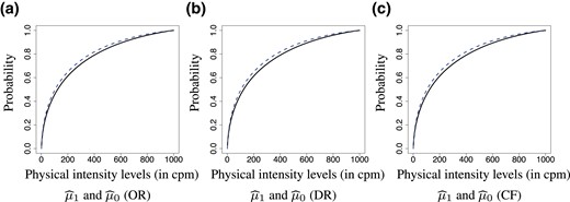
Panel (a), (b), and (c) plots μ^1 (black solid line) and μ^0 (blue dashed line) estimated by OR, DR, and CF, respectively.

Figure 3.

Panel (a), (b), and (c) plots ${\hat{μ}}_{1}$ (black solid line) and ${\hat{μ}}_{0}$ (blue dashed line) estimated by OR, DR, and CF, respectively.

Open in new tab Download slide

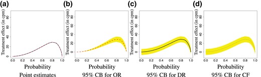
To quantify the size of the treatment effect, we take the difference between ${\hat{μ}}_{1}^{- 1}$ and ${\hat{μ}}_{0}^{- 1}$ ⁠, corresponding to the difference in quantiles of the mean potential outcomes μ₁ and μ₀. To quantify the uncertainty of these estimates, we plot the corresponding $95 %$ confidence bands in Figure 4b–d, where the confidence bands for the doubly robust and cross-fitting estimators were obtained using our asymptotic results presented in Theorems 3 and 4, and the confidence band for the outcome regression estimator was obtained using the conventional linear regression confidence interval for the slope coefficient corresponding to the exposure A. As expected, the estimation results from the three methods are very close to each other, and the OR method has the tightest confidence band among the three methods.

Figure 4.

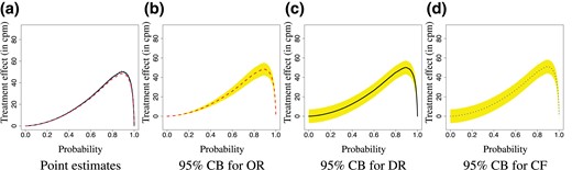
Difference in quantiles estimates with the OR (red dashed), DR (black solid), and CF (blue dotted) estimators: point estimates and 95% confidence bands.

Open in new tab Download slide

One can see from Figure 4 that the effect of marriage on physical activity level is significant at the 0.05 level. One can also get the causal effect on individual quantiles from these plots. For example, according to the DR estimation results, on average, marriage improves the median physical intensity level by 19.1 (95% CI = [12.1, 26.1]) cpm. Due to Theorem 1, this effect may be interpreted on both the population and individual levels. On the population level, this means that marriage improves the median of ‘average’ (in the sense of Wasserstein barycentre) physical intensity level by 19.1 cpm. On the individual level, this means that the average improvement on the median physical intensity level is 19.1 cpm. We also estimate the Wasserstein distance between ${\hat{μ}}_{1}^{D R}, {\hat{μ}}_{0}^{D R}$ ⁠, $W_{2} ({\hat{μ}}_{1}^{D R}, {\hat{μ}}_{0}^{D R}) = ‖ {\hat{Δ}}^{{\hat{μ}}_{0}^{D R}, D R} ‖_{{\hat{μ}}_{0}^{D R}}$ ⁠, and the estimate is 27.6 cpm (95% CI: [24.0, 31.2]).

One may also be interested in predicting the unobserved potential outcome for a particular individual. As an illustration, we estimate Y_i(1) for Subject 31144, who was unmarried so Y₃₁₁₄₄ = Y₃₁₁₄₄(0). Recall that $Δ_{i}^{Y_{i} (0)} = T_{i} - id$ ⁠. We first estimate the individual causal effect map for Subject 31144 using the average causal effect map with reference distribution ${\hat{Y}}_{31144} :$ ${\hat{T}}_{31144} = {\hat{Δ}}^{{\hat{Y}}_{31144}} + id,$ the latter being estimated using the DR method. We then apply the individual causal transport map to his empirical CDF to obtain ${\hat{Y}}_{31144} (1)$ plotted in Figure 5b. From this, one may obtain, for example, getting married would raise his mean physical activity from 144.5 cpm to 166.3 cpm (95% CI: [159.5, 173.7]).

Figure 5.

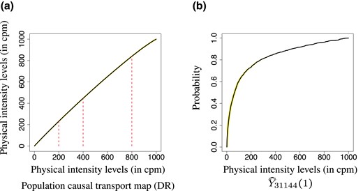
Panel (a) plots the DR estimate of population causal transport map, superimposed with the 95% confidence band; Panel (b) plots the DR estimate of counterfactual outcome Y(1) with 95% confidence band for individual 31144, who was unmarried so that Y₃₁₁₄₄ = Y₃₁₁₄₄(0).

Open in new tab Download slide

We also compare our adjusted estimates with the results where we do not adjust for the observed confounders age and gender. In particular, we apply the OR, DR, and CF estimators for estimating the average treatment effect $Δ^{λ}$ ⁠. We plot these estimates and the corresponding $95 %$ confidence bands in Figure 6. One can see the treatment effect is attenuated without adjusting for age and gender.

Figure 6.

Difference in quantiles estimates with the OR (red dashed), DR (black solid), and CF (blue dotted) estimators when we do not adjust for observed confounders age and gender: point estimates and 95% confidence bands.

Open in new tab Download slide

7 Discussion

In this paper, we study causal inference for distribution functions that reside in a Wasserstein space. We propose novel definitions of causal effects and develop doubly robust estimation procedures for estimating these effects under the assumption of no unmeasured confounding. It would be interesting to extend classical causal inference methods for dealing with unmeasured confounding, such as the instrumental variable methods (e.g., Ogburn et al., 2015; Wang & Tchetgen Tchetgen, 2018) to this setting.

To the best of our knowledge, ours is the first formal study of causal effects for outcomes defined in a nonlinear space. As such, we have only considered a leading special case of nonlinear spaces. There are many other data objects from nonlinear spaces that we do not consider in this paper. For example, the Wasserstein spaces of probability distributions on higher dimensional Euclidean spaces exhibit structures different from $W_{2} (I)$ and thus pose new challenges for causal inference on such spaces. We also note that although the Wasserstein space $W_{2} (I)$ is not a Riemannian manifold (Bigot et al., 2017), it can be endowed with a Riemannian structure, including the tangent space and Riemannian logarithmic map. In particular, let cl(S) denote the closure of set S. With a continuous reference distribution λ, the space $T_{λ} W_{2} (I) = c l {k (υ^{- 1} \circ λ - id) : υ \in W_{2} (I), k \in R^{+}}$ can be viewed as the tangent space of $W_{2} (I)$ at λ, and the mapping $υ \mapsto υ^{- 1} \circ λ - id$ can be viewed as the Riemannian logarithmic map at λ (Ambrosio et al., 2004). From this perspective, with the notation $L_{λ} υ = υ^{- 1} \circ λ$ ⁠, the individual causal effect maps can be written as $Δ_{i}^{λ} = L_{λ} Y_{i} (1) - L_{λ} Y_{i} (0) = {L_{λ} Y_{i} (1) - id} - {L_{λ} Y_{i} (0) - id},$ so they may be equivalently defined as the contrasts between the Riemannian logarithmic maps of distribution functions Y_i(1) and Y_i(0). By Theorem 1, the average causal effect map may then be equivalently defined as $Δ^{λ} = E (L_{λ} Y (1) - id) - E (L_{λ} Y (0) - id) .$ These connections allow one to extend the proposed definition of causal effect from random distributions to random elements residing on a Riemannian manifold; see Srivastava and Klassen (2016) for concepts and tools of Riemannian manifolds that are relevant to statistics.

Another interesting venue for future research is the study of efficiency theory with distribution-valued outcomes. It is well known that the classical doubly robust and cross-fitting estimators (Chernozhukov et al., 2018; Robins et al., 1994) are both doubly robust and locally semiparametric efficient. In Theorems 3 and 4, we establish double robustness of our proposed doubly robust and cross-fitting estimators. On the other hand, to establish semiparametric efficiency of these proposed estimators, one needs to extend semiparametric efficiency theory to accommodate distribution-valued outcomes that reside in infinite-dimensional functional spaces. This will be developed in a separate paper.

Supplementary material

Supplementary material are available at Journal of the Royal Statistical Society: Series B online.

Data availability

The supplementary file contains some auxiliary results, technical lemmas, and proofs for all the theorems. R code to reproduce the simulation studies and data analysis can be found in the repository https://github.com/kongdehanstat/causaldistributionfunction. The data analysed in Section 6 is available at https://wwwn.cdc.gov/nchs/nhanes/ContinuousNhanes/Default.aspx?BeginYear=2005.

References

Agueh

M.

, &

Carlier

G.

(

2011

).

Barycenters in the Wasserstein space

.

SIAM Journal on Mathematical Analysis

,

43

(

2

),

904

–

924

. https://doi.org/10.1137/100805741

Google Scholar

Crossref

WorldCat

Ambrosio

L.

,

Gigli

N.

, &

Savaré

G.

(

2004

).

Gradient fows with metric and dierentiable structures, and applications to the Wasserstein space

.

Atti della Accademia Nazionale dei Lincei. Classe di Scienze Fisiche, Matematiche e Naturali. Rendiconti Lincei. Serie IX. Matematica e Applicazioni

,

15

(3-4),

327

–

343

.

Google Scholar

OpenURL Placeholder Text

WorldCat

Ambrosio

L.

,

Gigli

N.

, &

Savare

G.

(

2005

).

Gradient flows

.

Birkhäuser

.

Google Scholar

Google Preview

OpenURL Placeholder Text

WorldCat

Arjovsky

M.

,

Chintala

S.

, &

Bottou

L.

(

2017

).

Wasserstein generative adversarial networks. In International Conference on Machine Learning (pp. 214–223). PMLR

.

Bernton

E.

,

Jacob

P. E.

,

Gerber

M.

, &

Robert

C. P.

(

2019

).

Approximate Bayesian computation with the Wasserstein distance

.

Journal of the Royal Statistical Society: Series B (Statistical Methodology)

,

81

(

2

),

235

–

269

. https://doi.org/10.1111/rssb.12312

Google Scholar

Crossref

WorldCat

Bigot

J.

(

2020

).

Statistical data analysis in the Wasserstein space

.

ESAIM: Proceedings and Surveys

,

68

,

1

–

19

. https://doi.org/10.1051/proc/202068001

Google Scholar

Crossref

WorldCat

Bigot

J.

,

Gouet

R.

,

Klein

T.

, &

López

A.

(

2017

).

Geodesic PCA in the Wasserstein space by convex PCA

.

Annales de l’Institut Henri Poincaré, Probabilités et Statistiques

,

53

(1),

1

–

26

. http://dx.doi.org/10.1214/15-AIHP706

Google Scholar

Crossref

WorldCat

Bigot

J.

,

Imb

T. K.

, &

Imt

Enac

(

2012

).

Characterization of barycenters in the Wasserstein space by averaging optimal transport maps

.

ESAIM: Probability and Statistics

,

22

,

35

–

57

. https://doi.org/10.1051/ps/2017020

Google Scholar

Crossref

WorldCat

Chang

H.-W.

, &

McKeague

I. W.

(

2020

).

‘Nonparametric comparisons of activity profiles from wearable device data’, preprint

.

Chen

Y.

,

Lin

Z.

, &

Müller

H.-G.

(

2021

).

Wasserstein regression

.

Journal of the American Statistical Association

,

1

–

14

. https://doi.org/10.1080/01621459.2021.1956937

Google Scholar

OpenURL Placeholder Text

WorldCat

Chernozhukov

V.

,

Chetverikov

D.

,

Demirer

M.

,

Duflo

E.

,

Hansen

C.

,

Newey

W.

, &

Robins

J.

(

2018

).

Double/debiased machine learning for treatment and structural parameters

.

The Econometrics Journal

,

21

(

1

),

C1

–

C68

. https://doi.org/10.1111/ectj.12097

Google Scholar

Crossref

WorldCat

Courty

N.

,

Flamary

R.

,

Tuia

D.

, &

Rakotomamonjy

A.

(

2016

).

Optimal transport for domain adaptation

.

IEEE Transactions on Pattern Analysis and Machine Intelligence

,

39

(

9

),

1853

–

1865

. https://doi.org/10.1109/TPAMI.2016.2615921

Cuturi

M.

, &

Doucet

A.

(

2014

).

Fast computation of Wasserstein barycenters. In Proceedings of the 31st International Conference on Machine Learning (ICML) (Vol. 32)

. PMLR.

del Barrio

E.

,

Cuesta-Albertos

J. A.

,

Matrán

C.

, &

Rodríguez-Rodríguez

J. M.

(

1999

).

Tests of goodness of fit based on the L2-Wasserstein distance

.

Annals of Statistics

,

27

(

4

),

1230

–

1239

. https://doi.org/10.1214/aos/1017938923

Google Scholar

OpenURL Placeholder Text

WorldCat

Fournier

N.

, &

Guillin

A.

(

2015

).

On the rate of convergence in Wasserstein distance of the empirical measure

.

Probability Theory and Related Fields

,

162

(

3–4

),

707

–

738

. https://doi.org/10.1007/s00440-014-0583-7

Google Scholar

OpenURL Placeholder Text

WorldCat

Hernán

M.

, &

Robins

J.

(

2020

).

Causal inference: What if

.

Chapman & Hall/CRC

.

Google Scholar

Google Preview

OpenURL Placeholder Text

WorldCat

Ho

N.

,

Nguyen

X.

,

Yurochkin

M.

,

Bui

H. H.

,

Huynh

V.

, &

Phung

D.

(

2017

).

Multilevel clustering via Wasserstein means. In International Conference on Machine Learning (pp. 1501–1509). PMLR

.

Kim

Y.-H.

, &

Pass

B.

(

2017

).

Wasserstein barycenters over Riemannian manifolds

.

Advances in Mathematics

,

307

,

640

–

683

. https://doi.org/10.1016/j.aim.2016.11.026

Google Scholar

Crossref

WorldCat

King

A. C.

,

Kiernan

M.

,

Ahn

D. K.

, &

Wilcox

S.

(

1998

).

The effects of marital transitions on changes in physical activity: Results from a 10-year community study

.

Annals of Behavioral Medicine

,

20

(

2

),

64

–

69

. https://doi.org/10.1007/BF02884450

Neyman

J. S.

(

1923

).

On the application of probability theory to agricultural experiments. Essay on principles. Section 9. (Translated and edited by DM Dabrowska and TP Speed, Statistical Science (1990), 5, 465–480)

.

Annals of Agricultural Sciences

,

10

(4),

1

–

51

.

Google Scholar

OpenURL Placeholder Text

WorldCat

Ogburn

E. L.

,

Rotnitzky

A.

, &

Robins

J. M.

(

2015

).

Doubly robust estimation of the local average treatment effect curve

.

Journal of the Royal Statistical Society: Series B (Statistical Methodology)

,

77

(

2

),

373

–

396

. https://doi.org/10.1111/rssb.12078

Panaretos

V. M.

, &

Zemel

Y.

(

2019

).

Statistical aspects of Wasserstein distances

.

Annual Review of Statistics and Its Application

,

6

(

1

),

405

–

431

. https://doi.org/10.1146/annurev-statistics-030718-104938

Google Scholar

Crossref

WorldCat

Petersen

A.

, &

Müller

H.-G.

(

2016

).

Functional data analysis for density functions by transformation to a Hilbert space

.

The Annals of Statistics

,

44

(

1

),

183

–

218

. https://doi.org/10.1214/15-AOS1363

Google Scholar

Crossref

WorldCat

Ramsay

J. O.

, &

Silverman

B. W.

(

2005

).

Functional data analysis

.

Springer

.

Robins

J. M.

,

Rotnitzky

A.

, &

Zhao

L. P.

(

1994

).

Estimation of regression coefficients when some regressors are not always observed

.

Journal of the American Statistical Association

,

89

(

427

),

846

–

866

. https://doi.org/10.1080/01621459.1994.10476818

Google Scholar

Crossref

WorldCat

Rosenbaum

P. R.

, &

Rubin

D. B.

(

1983

).

The central role of the propensity score in observational studies for causal effects

.

Biometrika

,

70

(

1

),

41

–

55

. https://doi.org/10.1093/biomet/70.1.41

Google Scholar

Crossref

WorldCat

Rubin

D. B.

(

1974

).

Estimating causal effects of treatments in randomized and nonrandomized studies

.

Journal of Educational Psychology

,

66

(

5

),

688

–

701

. https://doi.org/10.1037/h0037350

Google Scholar

Crossref

WorldCat

Rubin

D. B.

(

1980

).

Comment

.

Journal of the American Statistical Association

,

75

(371),

591

–

593

. https://doi.org/10.2307/2287653

Google Scholar

OpenURL Placeholder Text

WorldCat

Santambrogio

F.

(

2015

).

Optimal transport for applied mathematicians

.

Birkhäuser

.

Schiebinger

G.

,

Shu

J.

,

Tabaka

M.

,

Cleary

B.

,

Subramanian

V.

,

Solomon

A.

,

Gould

J.

,

Liu

S.

,

Lin

S.

,

Berube

P.

,

Lee

L.

,

Chen

J.

,

Brumbaugh

J.

,

Rigollet

P.

,

Hochedlinger

K.

,

Jaenisch

R.

,

Regev

A.

, &

Lander

E. S.

(

2019

).

Optimal-transport analysis of single-cell gene expression identifies developmental trajectories in reprogramming

.

Cell

,

176

(

4

),

928

–

943.e22

. https://doi.org/10.1016/j.cell.2019.01.006

Sommerfeld

M.

, &

Munk

A.

(

2018

).

Inference for empirical Wasserstein distances on finite spaces

.

Journal of the Royal Statistical Society: Series B (Statistical Methodology)

,

80

(

1

),

219

–

238

. https://doi.org/10.1111/rssb.12236

Google Scholar

Crossref

WorldCat

Srivastava

A.

, &

Klassen

E. P.

(

2016

).

Functional and shape data analysis

. (Vol.

1

).

Springer

.

Troiano

R. P.

,

McClain

J. J.

,

Brychta

R. J.

, &

Chen

K. Y.

(

2014

).

Evolution of accelerometer methods for physical activity research

.

British Journal of Sports Medicine

,

48

(

13

),

1019

–

1023

. https://doi.org/10.1136/bjsports-2014-093546

Tudor-Locke

C.

,

Camhi

S. M.

, &

Troiano

R. P.

(

2012

).

Peer reviewed: A catalog of rules, variables, and definitions applied to accelerometer data in the National Health and Nutrition Examination Survey, 2003–2006

.

Preventing Chronic Disease

,

9

,

E113

. https://doi.org/10.5888/pcd9.110332

Google Scholar

PubMed

OpenURL Placeholder Text

WorldCat

Verdinelli

I.

, &

Wasserman

L.

(

2019

).

Hybrid Wasserstein distance and fast distribution clustering

.

Electronic Journal of Statistics

,

13

(

2

),

5088

–

5119

. https://doi.org/10.1214/19-EJS1639

Google Scholar

Crossref

WorldCat

Wang

L.

, &

Tchetgen Tchetgen

E.

(

2018

).

Bounded, efficient and multiply robust estimation of average treatment effects using instrumental variables

.

Journal of the Royal Statistical Society: Series B (Statistical Methodology)

,

80

(

3

),

531

–

550

. https://doi.org/10.1111/rssb.12262

Zhang

C.

,

Kokoszka

P.

, &

Petersen

A.

(

2020

).

‘Wasserstein autoregressive models for density time series’, arXiv, arXiv:2006.12640, preprint: not peer reviewed

.

Zhou

H.

,

Lin

Z.

, &

Yao

F.

(

2021

).

‘Intrinsic Wasserstein Correlation Analysis’, arXiv, preprint: not peer reviewed

.

Zhu

C.

, &

Müller

H.-G.

(

2021

).

‘Autoregressive optimal transport models’, arXiv, preprint: not peer reviewed

.

Footnotes

https://wwwn.cdc.gov/nchs/nhanes/ContinuousNhanes/Default.aspx?BeginYear=2005.

Author notes

Conflict of interest None declared.

This article is published and distributed under the terms of the Oxford University Press, Standard Journals Publication Model (https://dbpia.nl.go.kr/pages/standard-publication-reuse-rights)

Download all slides

Month:	Total Views:
March 2023	394
April 2023	272
May 2023	121
June 2023	68
July 2023	82
August 2023	67
September 2023	41
October 2023	59
November 2023	36
December 2023	47
January 2024	48
February 2024	64
March 2024	56
April 2024	182
May 2024	149
June 2024	76
July 2024	156
August 2024	133
September 2024	145
October 2024	137
November 2024	142
December 2024	130
January 2025	123
February 2025	119
March 2025	120
April 2025	104
May 2025	62

Article Contents

Causal inference on distribution functions

Abstract

1 Introduction

Physical activities

2 Background

2.1 The potential outcomes framework

2.2 Causal effect identification and estimation

Ignorability

Positivity

2.3 Wasserstein space

3 Causal inference on distribution functions

3.1 Definition of causal effects

Difference in quantiles

Causal transport maps

3.2 Properties of causal effect maps

3.3 Identification and estimation

4 Asymptotic properties

5 Simulation studies

6 Data application

7 Discussion

Supplementary material

Data availability

References

Footnotes

Author notes

Supplementary data

Citations

Views

Altmetric

Email alerts

Citing articles via

Latest

Most Read

Most Cited

Article Contents

Causal inference on distribution functions Free

Abstract

1 Introduction

Physical activities

2 Background

2.1 The potential outcomes framework

2.2 Causal effect identification and estimation

Ignorability

Positivity

2.3 Wasserstein space

3 Causal inference on distribution functions

3.1 Definition of causal effects

Difference in quantiles

Causal transport maps

3.2 Properties of causal effect maps

3.3 Identification and estimation

4 Asymptotic properties

5 Simulation studies

6 Data application

7 Discussion

Supplementary material

Data availability

References

Footnotes

Author notes

Supplementary data

Citations

Views

Altmetric

Email alerts

Citing articles via

Latest

Most Read

Most Cited

This Feature Is Available To Subscribers Only

Causal inference on distribution functions