


Abstract
We compare causal effects of forward guidance about future interest rates on households’ expectations of inflation and nominal mortgage rates to the effects of communication about inflation in a randomized control trial using more than 20,000 U.S. consumers in the Nielsen Homescan Panel. We elicit consumers’ expectations, and then provide 22 different forms of information regarding past, current, and/or future interest rates and inflation. Information treatments about current or future interest rates all have similar and offsetting effects on interest rate and inflation expectations, yielding limited pass-through into perceived real rates. Information about mortgage rates has much more powerful effects on interest rate perceptions, with no offsetting effects on inflation expectations, thereby delivering much larger changes in perceived real rates. Revisions in perceived real rates causally lead to changes in the ex-post purchases of durable goods by households.
“Under the empirically reasonable assumption that what matters for aggregate spending is the entire expected path of short-term rates rather than just the current level, [forward guidance] enables the Fed to provide substantial additional accommodation during zero lower bound episodes. The strategy also potentially supports aggregate demand by raising inflation expectations, thereby lowering real long-term rates relative to a Taylor Rule type baseline.” Janet Yellen, September 2018.1
“After all, it is the everyday economic decisions of people and companies that we seek to influence with our policy and communication. If our language is not accessible, our policy will be less effective.” Christine Lagarde, February 2020.2
“The limits to forward guidance depend on what the public understands, and what it believes. In normal times, the general public does not pay much attention to central bank statements, so robust policies should be designed to be effective even if they are followed closely only by financial market participants. ... policymakers must communicate consistently and intelligibly.” Ben Bernanke, January 2020.3
1. Introduction
As monetary policymakers in many advanced economies pushed short-term interest rates to zero both during the financial crisis and during the recent COVID-19 pandemic, attention quickly turned to other tools that could be used to further stimulate economic activity. Along with quantitative easing, forward guidance about the path of future interest rates became one of the main tools that central banks developed to address the exceptional circumstances they have been facing. Understanding how forward guidance affects economic outcomes is therefore a central question. But because the mechanism of forward guidance is via expectations and these are not readily observable, it has been difficult to establish how announcements about the future actually affect individual economic actors.
In this paper, we implement a large-scale randomized control trial (RCT) on a representative sample of about 20,000 U.S. consumers to whom we provide, in a randomized fashion, different pieces of information about the evolution of future interest rates as well as about past and current policy rates and inflation. This RCT approach provides a transparent way to assess whether the exogenous provision of information about interest rates and inflation changes households’ economic expectations. The large scale of the experiment allows us to characterize in unprecedented detail how the magnitude of the treatment as well as the time horizon of the announcement affects the size of consumers’ forecast revisions and how they change their views about different economic variables (e.g. long-term interest rates vs. inflation). We can also assess whether the resulting variation in perceived real interest rates of households changes their actual spending decisions on both durables and non-durables.
Households’ expectations play a central role in the transmission of forward guidance into economic outcomes through several channels. Forward guidance operates in part via financial markets, which determine changes in long-term nominal interest rates. The pass-through of these interest rates into consumption and saving decisions then determines how large the effect of forward guidance through the financial markets channel is. It is well documented that households exhibit considerable inertia in their borrowing decisions (e.g. in refinancing their fixed rate mortgages in a period of declining interest rates; see Campbell 2006; Andersen et al. 2020) . Recently, D’Acunto et al. (2018b) find that many households do not adjust their mortgage choices to changes in interest rates. We provide new evidence on households’ perceptions of market interest rates and how they respond to different types of information that speaks directly to the potential strength of this channel.
An additional channel through which forward guidance should stimulate spending is via the inflation expectations of households: If households anticipate larger price increases in the future, then they have an incentive to spend more today. We show that in standard New Keynesian models this is often the most powerful transmission channel of forward guidance. However, prior work should give one pause before placing much faith in this channel. D’Acunto, Hoang, and Weber (2022), for example, show that European households did not adjust their inflation expectations in the months bracketing the initial forward guidance announcement by the European Central Bank (ECB). Our results speak to the potential strength of this additional channel by characterizing how inflation expectations respond to different types of information about current and future interest rates.
We document a number of new results from this large-scale experiment. First, prior to any information treatment, we find that households’ knowledge about market interest rates is limited: The cross-sectional dispersion in their beliefs about the level of the 30-year mortgage rate is as high as previously documented for their beliefs about inflation (e.g. Coibion, Gorodnichenko, and Weber 2022). This lack of knowledge on the part of many consumers about one key interest rate is suggestive that pass-through of forward guidance from financial markets to households may be limited. Second, we find that the provision of information to households about current, past, and future policy rates of the Federal Reserve has only limited effects on households’ perceptions of both current and future market interest rates even though they result in large actual changes in mortgage rates (Eichenbaum, Rebelo, and Wong 2022). Households place a weight of 80%–90% on their prior beliefs about interest rates when they receive signals about past, current, or future policy rates. This again suggests that communication about policy rates is unlikely to lead to large changes in household spending. Third, providing information about current, past, and future policy rates leads households to revise their inflation expectations by large amounts: those with initially high inflation expectations lower them while those with low expectations raise them. Households place a weight of only 10%–20% on their prior inflation expectations when provided with information about policy rates. Despite the limited effect of information treatments about policy interest rates on the expected interest rates of households, their perceived real interest rates still change due to the sensitivity of their inflation expectations: The implied weight on their prior beliefs about real rates relative to the control group is on the order of 40%–60% depending on the specific information treatment. We then confirm that exogenous variation in the perceived real interest rates of households affects their subsequent durable goods purchases.
We find even more promising results for communication strategies focusing on long-term market interest rates themselves. One of our information treatments consists of informing households about the current 30-year mortgage rate. This treatment leads to a very strong response in households’ perceptions of the mortgage rate (an almost complete convergence in beliefs to the provided information), which extends into households’ expectations about future long-term rates as well. In addition, and unlike what was found with either policy rate or inflation rate treatments, providing information to households about the mortgage rate leads to almost no revision in their inflation expectations. The resulting effect on their perceived real interest rate is much larger than what we observe with other treatments: Implied weights on prior beliefs about real rates are only about 10%–30%, indicating that this treatment leads to large average revisions in perceived real interest rates. Consistent with Angeletos and Sastry (2021), this result implies that communication about the target (in this case, the mortgage interest rate) may be a more effective form of forward guidance than communication about the policy rate. And since we also show below that exogenously generated changes in households’ perceived real interest rates affect households’ ex-post purchases of durable goods, communication about market interest rates could provide a much more powerful way of stimulating consumption than forward guidance about future policy rates.
To measure how households’ expectations change in response to information treatments, we first elicit households’ expectations on a host of variables including inflation and nominal mortgage rates. Subsequently, we provide information treatments to households, and finally, elicit household expectations again, both shortly after the treatment as well as after 3 and 6 months. The latter allows us to characterize how persistent the effects of different information treatments are on households’ expectations. We document that treatments about policy rates and inflation have somewhat persistent effects, present after 3 months but significantly dampened after 6 months. In contrast, the treatment involving mortgage rates dissipates much more rapidly.
Because our survey has such a large cross-section, we can consider an exceptionally large number of different treatments relative to previous work and perform multiple comparisons. Specifically, we vary (i) the variable on which we provide information: policy rates, inflation, and mortgage rates; (ii) the horizon over which we provide information: current, past, and future periods up to 3 years into the future and for the longer run; and (iii) the interest rate trajectories: central tendency, upper range, and lower range. This variety in treatments is the source of our ability to identify in such detail what types of information affect households’ beliefs most and which dimensions are less important. For example, we find very little effect stemming from the time horizon of information about policy rates: Whether the information is only about current rates or extends to several years out seems to have little marginal effect on beliefs. The fact that households do not adjust their expectations to a larger extent to information beyond 1 year provides empirical support to theories that model decision makers with limited capacity to collect and process information: for example, limited planning horizons (Woodford 2018), bounded rationality (Gabaix 2020), level-k thinking (Farhi and Werning 2019), or lack of common information (Angeletos and Lian 2018). While the exact micro foundations differ across studies, they share the feature that agents with limited abilities are not necessarily more responsive to information in the far future relative to information about the current and immediate future.
The recent focus of policymakers on forward guidance originates in part from the fact that conventional monetary policy was no longer feasible once policy rates hit the effective lower bound. One potential caveat of our survey could therefore be that we implemented it during a period in which the U.S. had already normalized interest rates to positive levels. We believe our findings still provide important insights for several reasons. First, many households have expectations and perceptions of current interest rates that deviate significantly from the actual rates so their reaction in the survey is informative about how individuals would actually react to a forward guidance announcement. Second, the use of forward guidance long predates the Great Recession and the extent to which forward guidance affects financial markets has been studied not only during the zero bound but also outside of it (Gürkaynak et al. 2005). Third, central bankers anticipate that forward guidance and other communications-based policies can become a more conventional tool in the future (Blinder et al. 2017). Fourth, to the extent we exploit cross-sectional variation, we keep constant the level of interest rates and exploit differences in the reaction of individuals to different information treatments. This cross-sectional variation, because it identifies the weight households place on their priors, nonetheless also speaks to the weight that households place on new information and therefore to the first-round effects of communication strategies.
Randomized controlled trials have recently become more common in macroeconomics (e.g. Binder and Rodrigue 2018; Armona, Fuster, and Zafar 2019; Coibion et al. 2020a, 2021; D’Acunto et al. 2020; Roth and Wohlfart 2020). Following the design of research in applied micro and development, these papers typically study how randomized treatments affect individuals’ expectations and decisions in domains that are directly affected by the treatments. Yet, in macroeconomic contexts, feedback effects, general equilibrium effects, and the expectations on how other aggregate variables move in response to the treatment are important for the overall response of individuals. A central innovation in our survey design is the fact that we can jointly study the response of several economic expectations to our different treatments to better predict how individuals form expectations jointly and how they might react to actual announcements by central banks on how the future path of policy rates or inflation might evolve. Furthermore, we study how information about past, current, and future policy rates influence expectations of households and contrast these responses with those of households who are informed about inflation, a powerful force for moving households’ expectations about macroeconomic variables (e.g. Coibion, Gorodnichenko, and Weber 2022) as well as a strong determinant of households’ consumption (e.g. D’Acunto et al. 2016; Coibion et al. 2019) in the U.S.4
Our paper is closely related to an extensive body of work on the effect of forward guidance (Campbell et al. 2012; Del Negro et al. 2015; Andrade and Ferroni 2021). However, we differ from this work along a number of dimensions. First, much of this work (e.g. Chodorow-Reich 2014) has concentrated on how forward guidance affects financial markets and nominal interest rates of different maturities. We complement this literature by providing evidence on how households respond to information about interest rates. We show, for example, that providing information about future interest rates changes not just the perceived path of nominal rates but also inflation expectations, so that the pass-through to households’ real interest rates is much less than one-for-one. In addition, households may be sensitive not just to the level of long-term interest rates but also to their expected path: The timing of durable goods purchases is likely to depend on whether households expect interest rates to rise or fall in the future because purchases of durable goods have a very high intertemporal elasticity of substitution (e.g. House and Shapiro 2008). We regard our results on the response of households’ interest and inflation expectations as complementary to earlier work focusing on financial markets by helping to identify additional channels through which forward guidance shapes economic outcomes. Because households’ income expectations could also change in response to forward guidance, our results should not be interpreted as necessarily fully characterizing the response of households, and other expectations channels could also be important.5
Another strand of literature focuses on the aggregate effects of forward guidance, primarily using time series analysis (e.g. Swanson 2021; see Bhattarai and Neely 2012 for a survey). This research is of direct use in measuring how the economy responds to forward guidance, but it does not speak directly to the underlying mechanisms at work. Our approach is complementary: We are able to identify how households’ expectations and spending respond to information about current and future interest rates, but are unable to speak directly to the general equilibrium effects that would obtain were all households to respond in a similar fashion. However, by more precisely identifying the mechanisms, the horizon over which forward guidance operates, and the variable which central banks give guidance about, we hope that our work can be used to differentiate between and quantify models of forward guidance, which in turn can then be used for policy analysis and counterfactuals.
A recent strand of the theoretical literature develops models that limit the power of forward guidance either through deviations from full information rational expectations (Angeletos and Lian 2018; Woodford 2018; Farhi and Werning 2019; Gabaix 2020) or via introducing market incompleteness and constraints (Werning 2015; McKay et al. 2016; Kaplan et al. 2018; Hagedorn et al. 2019). We empirically add to this literature and study how individuals adjust their expectations to news about interest rates and inflation, how they adjust their consumption choices, and heterogeneity in the responses.
Our paper also relates to a much broader literature on central bank communication and how this communication shapes household expectations and decision-making. This literature has emphasized two general stylized facts for advanced economies. First, households (and firms) are often inattentive to policy and relatively uninformed about macroeconomic aggregates. Second, despite this inattention, households’ expectations about future aggregate conditions affect their decisions (see Coibion et al. 2020b; Weber et al. 2022; D’Acunto et al. 2022a for surveys of this literature). The results in this paper corroborate these two stylized facts but do so in the specific context of forward guidance. This growing body of evidence supports the recent interest among policymakers in rethinking their communication strategies with the public and suggests a need for more research to better understand the link between policy announcements and the decision-making process of economic agents.
Finally, some features of our approach are worth clarifying. First, most households do not actively follow central bank announcements (Lamla and Vinogradov 2019), even when major policy changes are made (Coibion et al. 2020a). In our survey experiment, we focus on an intensive margin of central bank communication, that is, we provide different information to agents and study which message is most effective in moving expectations, but we cannot speak to the extensive margin of information acquisition. Hence, our results on the effect of communication on expectations inform policymakers on the potential power of forward guidance to the extent they are able to reach consumers with their communication. Second, actual forward guidance announcements often provide additional context on the state of the economy, the economic outlook, and potential state dependence in the guidance such as a level of unemployment rate that has to be reached before considering interest rate changes. Previous work (Coibion, Gorodnichenko, and Weber 2022) finds that households revise their expectations similarly regardless of whether they only receive summary statistics for inflation or policy rates (as we provide here) or whether they are provided with substantially more details from actual policy statements. Third, forward guidance in practice is often about the future path of policy rates. We provide information not just about future rates but also about current and past interest rates, as well as on inflation and mortgage rates, because no systematic evidence exists so far on which form of guidance is most powerful in shaping individuals’ expectations. Policy rates are not directly relevant for most consumer decisions. Mortgage rates, on the other hand, are an important transmission channel of monetary policy (Wong 2020). Given that most mortgages in the U.S. are fixed rate mortgages, households have an incentive to be informed about the evolution of these rates to determine refinancing decisions (Berger et al. 2021; Eichenbaum et al. 2022). Last, inflation expectations are a key determinant of households’ saving and consumption decisions and, in New Keynesian models, forward guidance often operates primarily through inflation expectations.
2. Expectations and Consumption
A common narrative used by policymakers to describe how forward guidance affects household consumption is as follows: Forward guidance about future short-term rates will lower long-term rates, households will then reduce their saving and increase their spending while their inflation expectations remain well-anchored. We will refer to this as the “policy narrative”. In the context of the equation above, this narrative is built on the idea that forward guidance leads to a change in the long-term rate |$(di_t^m)$| , that households observe and respond to market rates |$(di_t^{hh}=di_t^m)$|, and that “well-anchored” inflation expectations are stable, that is, |$d(\sum _{j=0}^{\infty }E_t^{hh}\pi _{t+j+1})\approx 0$|. In short, the change in consumption from the policy narrative is |$dc_t^{ {pol}}=-\sigma di_t^m$|. In this narrative, all that is needed to evaluate the effect of forward guidance on consumption is the degree to which financial markets responded to the announcement, which is summarized by the response of the long-term nominal interest rate.
In standard New Keynesian models, the effect of forward guidance is generally quite large and certainly larger than what is implied by the policy narrative. With full-information rational expectations, household expectations of the long-rate are identical to the market rate, so |$i_t^m-i_t^{hh}=0$| and pass-through of changes in market interest rates into spending is complete. In addition, to the extent that forward guidance should induce higher inflation in subsequent periods and households anticipate this |$(d(\sum _{j=0}^{\infty }E_t^{hh}\pi _{t+j+1})> 0)$|, the expected inflation channel will also be present. Thus, |$dc_t^{NK}=-\sigma di_t^{m}+\sigma d(\sum _{j=0}^{\infty }E_t^{hh}\pi _{t+j+1})$|. Importantly, it is the inflation expectations of households, not of financial markets, which magnifies the effect of forward guidance on consumption decisions in standard macroeconomic models. Understanding how these household inflation expectations respond in practice therefore can help explain how much forward guidance affects economic outcomes.
To illustrate how either channel can dominate in driving the response of consumption, we plot responses to different types of monetary shocks in the benchmark Smets and Wouters (2007) model in Figure 1. The first such shock is a standard contemporaneous expansionary 25 basis points monetary policy shock. The associated persistent decline in the policy rate implies that the contemporaneous long-term (10-year) interest rate falls on impact (by 0.04% points) while expected inflation rises (by 0.03% points per year over 10 years), so that the real long-term interest rate falls sharply due to both channels, leading to a rise in consumption. With forward guidance shocks, however, the expected inflation channel becomes more important. For example, Figure 1 plots the effects of pre-announced expansionary monetary shocks 5 and 9 quarters later, assuming the policy rate is unconstrained before. The expected decline in future short-term rates leads to a rise in expected inflation and a boom in current activity. These announcements also induce a sharp rise in short-term interest rates before the monetary shocks are realized. In these cases, the contemporaneous long-term interest rate rises following the forward guidance announcement. The contemporaneous increase in consumption is therefore driven by the persistent rise in households’ expectations of future inflation. In this case, focusing on how long-term nominal interest rates set in financial markets responded to this shock would mischaracterize the effect on consumption.
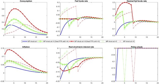
Response to current and anticipated policy shocks in the baseline Smets–Wouters model.
Notes: The figure plots impulse responses to different monetary shocks in the baseline Smets and Wouters (2007) model. The model uses parameter values estimated in Smets and Wouter (2007). “MP shock at time t” is the case of a 25 basis point shock to the Taylor rule happening contemporaneously (at time 1). “MP shock at time t|$+$|5(t|$+$|9)” is the case in which a 25 basis point expansionary monetary shock is pre-announced 1 year (2 years) prior, that is, the announcement is made at time 1 but the shock only occurs in quarter 5 (9). “MP shock at time t|$+$|5 (fixed FFR until t|$+$|4)” is the case of a 25 basis point monetary shock happening in quarter 5 but pre-announced at time 1, with the policy rate made to be fixed until the shock is realized. “MP shock at time t|$+$|9 (fixed FFR until t|$+$|8)” is analogous to previous case but with a 2-year gap between announcement and policy shock.
Even if we assume that policy rates are fixed prior to the pre-announced shock (also shown in Figure 1) so that the long-term interest rate must fall on impact, then the expected inflation effect quantitatively drives the behavior of consumption. For example, when the shock is pre-announced by 1 year, the long-term (10-year) nominal interest rate falls by only 1 basis point, while the change in expected inflation is six times larger. The effect of forward guidance on consumption in a standard macroeconomic model therefore hinges on households’ expectations of future inflation, not just the response of long-term nominal interest rates set in financial markets.
Moving beyond full-information models, one can also allow for the possibility that changes in market interest rates are not fully incorporated into households’ perceptions of these rates (i.e. |$di_t^{hh}\ne di_t^m$|). In that case, changes in consumption depend on how households’ perceptions of market rates change with forward guidance, as well as their inflation expectations |$dc_t^{{gen}}=-\sigma di_t^{hh}+\sigma d(\sum _{j=0}^{\infty }E_t^{hh}\pi _{t+j+1})$|. Abstracting from general equilibrium effects, forward guidance can have larger effects than in the standard model if household expectations over-react relative to markets (as in e.g. Bordalo et al. 2020). If instead households are very inattentive and do not change their perceptions of interest rates and their inflation expectations at all, then forward guidance can be impotent in affecting consumption |$(dc_t^{{gen}}=0$|) regardless of what happens in financial markets.
3. Data and Survey Design
This section describes our survey design to elicit expectations, the various treatments, and provides descriptive statistics for a range of expectations and perceptions. We first detail the Nielsen Homescan panel on which we run the survey and provide more information on the structure of the survey.
3.1. Nielsen Panel
In March, June, and September of 2019, we fielded three waves of the Chicago Booth Expectations and Communications Survey inviting participation by all household members in the Kilts–Nielsen Consumer Panel (KNCP). The KNCP represents a panel of approximately 80,000 households that report to Nielsen (i) their static demographic characteristics, such as household size, income, ZIP code of residence, and marital status, and (ii) the dynamic characteristics of their purchases, that is, which products they purchase, at which outlets, and at which prices. Panelists update their demographic information at an annual frequency to reflect changes in household composition or marital status.
Nielsen attempts to balance the panel on nine dimensions: household size, income, age of household head, education of female household head, education of male household head, presence of children, race/ethnicity, and occupation of the household head. Panelists are recruited online, but the panel is balanced using Nielsen’s traditional mailing method. Nielsen checks the sample characteristics on a weekly basis and performs adjustments when necessary.
Nielsen provides households with various incentives to ensure the accuracy and completeness of the information they report. These incentives include monthly prize drawings, providing points for each instance of data submission, and engaging in ongoing communication with households. Panelists can use points to purchase gifts from a Nielsen-specific award catalog. Nielsen structures the incentives to not bias the shopping behavior of their panelists. The KNCP has a retention rate of more than 80% at the annual frequency. Nielsen validates the reported consumer spending with the scanner data of retailers on a quarterly frequency to ensure high data quality and filters households that do not report a minimum amount of spending over the previous 12 months.
3.2. Chicago Booth Expectations and Communication Survey
Nielsen runs surveys on a monthly frequency on a subset of panelists in the KNCP, the online panel, but also offers customized solutions for longer surveys. Retailers and fast-moving consumer-goods producers purchase this information and other services from Nielsen for product design and target-group marketing. At no point of the survey did Nielsen tell their panelists that the survey we fielded was a part of academic research which minimizes the concerns of survey demand effects (de Quidt et al. 2018).
In early 2019, we designed a customized survey consisting of 34 questions in total in cooperation with Nielsen, the Chicago Booth Expectations and Communication Survey. The survey also contains 22 different information treatments, one placebo treatment as well as one control group. Our survey design builds on the Michigan Survey of Consumers, the New York Fed Survey of Consumer Expectations (SCE), the Dutch National Bank’s Household Survey as well as D’Acunto et al. (2021b), Coibion, Gorodnichenko, and Weber (2022), and Coibion et al. (2020b).
Nielsen fielded the first wave of the survey in March of 2019. The survey sample was 92,982 households. 26,929 individuals (from 24,886 households) responded for a response rate of 26.80% and an average response time of 19 minutes and 35 seconds. The second and third waves consisted mostly of follow-up questions, with median response times of about 19 minutes and 28,580 unique respondents for the second wave (June 2019; 16,726 participated in the initial wave) and 15,912 unique respondents for the third wave (September 2019; 8,152 participated in the initial wave). Nielsen provides weights to ensure representativeness of the households participating in the survey. The response rate compares favorably with other ad-hoc surveys and is similar to other studies running surveys on Nielsen, such as D’Acunto et al. (2021b). For example, Qualtrics estimates an average response rate between 5 and 10% across their surveys (D’Acunto et al. 2022b).
The initial wave of the survey covers a wide range of questions. First, respondents are presented with a series of questions about their demographic characteristics, which are more detailed relative to the basic demographic information the KNCP provides. We collect information on employment status, current occupation, financial constraints, savings and portfolio choice, homeownership status, and past spending behavior in various categories, including expenses that are not covered in the KNCP, and we identify the primary shopper of the household among all the responding members (D’Acunto, Malmendier, and Weber 2019). Participants are then asked a sequence of questions about their perceptions and expectations of inflation. We follow the design in the SCE and ask specifically about inflation, because asking about prices might induce individuals to think about specific items whose prices they recall rather than about overall inflation (see Crump et al. 2022 for a recent paper using the SCE data). We first ask individuals about their perception of past inflation, that is, inflation over the previous 12 months. We then ask them about their expectations for 12-month-ahead inflation. We elicit a full probability distribution of expectations by asking participants to assign probabilities to different possible levels of the inflation rate. Finally, we also ask survey participants on their expectations regarding interest rates on a 30-years fixed rate mortgage at the end of 2019, 2020, 2021, and in the next 5–10 years. Subsequent waves largely follow the same structure. Hence, the follow-up surveys are primarily used to measure individuals’ perceptions and expectations of inflation and nominal mortgage rates.
3.3. Information Treatments
After respondents answered the initial set of questions in the first wave, they were assigned to one of 24 groups: a control group, one placebo treatment group, and 22 treatment groups. We designed the treatments to disentangle the effects of different possible types of forward guidance. We vary the target that is communicated: We not only communicate inflation forecasts or expected future policy rates but also vary the length of the forecast horizon, the exact information of the forecast, central tendency, upper range, or lower range, or all jointly, as well as different combinations. All future policy forecasts are taken from the Survey of Economic Projections submitted by Federal Open Market Committee (FOMC) members, which provide both central tendencies as well as a range of forecasts from FOMC members. In addition to information about future policy rates, some survey participants only received information about current/past rates. The latter treatments allow us to study the extent to which consumers might have differential responses to backward-looking versus forward-looking information. We also fielded a placebo treatment to differentiate true learning from spurious anchoring effects. Each group consists of approximately 1/24th of the total sample that received the survey and the treatments are randomly assigned. Online Appendix Table A.3 confirms that assignment of treatment was not predictable by respondents’ observable household and individual characteristics. Although the number of treatments is large and thus one may be concerned about inflated p-values due to multiple hypothesis testing, our sample size is so large and our estimates are so precise that p-values adjusted for multiple hypothesis testing are nearly identical to the conventional p-values.6
Our choice of treatments is motivated by a number of practical and theoretical considerations. Central banks often give forward guidance directly about the future path of their policy instrument, the Fed Funds Rate (FFR) in the U.S., with the goal of influencing contemporaneous long-term interest rates via the expectations hypothesis for interest rates, that is, changing financial market participants’ expectations of future short-term interest rates should be reflected in current long term interest rates. The transmission to the real economy then occurs because these long-term rates affect households’ and firms’ borrowing decisions and the purchase of durable goods and investment goods as the introductory quote by former Fed Chair Janet Yellen indicates.
Theoretically, forward guidance typically operates through affecting household expectations of inflation and the consumer Euler equation (Eggertson and Woodford 2003). Promises to keep interest rates low until after the end of the liquidity trap will be inflationary in the future and hence, households should already update upwards their inflation expectations today which during the liquidity trap period will translate into lower real rates and stimulate consumption. Therefore, we also directly provide treatments about the future path of interest rates and inflation to study whether forecasts for inflation or the path of interest rates are more effective in moving consumers’ expectations. Moreover, given that central banks often focus on a transmission mechanism through financial markets and household borrowing, we also directly study the reaction of individuals’ expectations regarding future mortgage rates and contrast the effects with the reaction of inflation expectations that are the focus in the academic literature and in virtually all models used by leading central banks.
Empirically, forward guidance appears to be less powerful than standard theory predicts, a phenomenon commonly referred to as the forward guidance puzzle (Del Negro et al. 2015; D’Acunto et al. 2022). Recent theoretical attempts (e.g. Angeletos and Lian 2018; Woodford 2018; Farhi and Werning 2019; Gabaix 2020) at resolving this puzzle that emerges in a representative agent New Keynesian model propose deviations from rational expectations as a possible resolution. While the exact microfoundations differ, they all attribute an important role to some form of limited cognition on the part of the consumer. These models attribute lower effectiveness of communication in the future on current day expectations to the fact that the agents in the model either do not plan that far into the future or they discount the information heavily. While we do not aim to disentangle the exact mechanism at play, the treatments with different horizons for the provided information can help assess whether these models are broadly consistent with the data.
Empirically, inflation expectations of households are widely dispersed suggesting some form of information friction. Given the evidence that many individuals are not well informed about the prevailing inflation rate and the possibility that agents form expectations adaptively, we also provided treatments that only informed households about the current inflation rate and policy rate. We then compare the reaction in forecasts to treatments about past, future or both pieces of information to better understand whether forward- or backward-looking expectations are a better description of expectations on average. The large cross-sectional component of our sample also allows us to study which type of consumers might have either forward- or backward-looking expectations.
Mortgage rates play a key role in the practice of monetary policy, yet central bankers typically do not directly communicate about mortgage rates or inflation (Wong 2020). D’Acunto et al. (2018b) find that many households do not change their borrowing behavior in response to changes in policy rates, possibly because they do not understand the implications of changes in policy rates on their borrowing rates. We therefore also directly provided some households with information about current mortgage rates with reference to a 30-year fixed rate mortgage (the most prevalent mortgage product in the U.S.). Thus, we examine whether communication about interest rates that are of direct interest to households might be more effective in guiding households’ expectations and decision-making.
Randomized control trials have gained interest in recent empirical macro studies but it is not yet clear how the provision of information on one macro variable jointly affects agents’ forecast for other variables that also affect economic behavior. Andre et al. (2022) find that many households differ in their reaction to fundamental shocks compared with the reaction of experts and models but nonetheless often revise expectations about different variables after structural shocks. Empirically, Coibion et al. (2019) find in an information provision experiment that households with exogenously higher inflation expectations lowered their spending on durables after the treatment because their overall economic outlook became more negative. Our setting allows us to study whether treatments about inflation or interest rates over different horizons might be a more promising communication tool for central banks to stimulate household spending because we can directly compare their effects on expectations but crucially also study in a systematic fashion how these treatments affect consumer expectations about inflation and mortgage rates jointly.
Finally, we also vary the trajectory for the future path of interest rates, that is, the high, central, and low forecasts for future interest rates. By varying the trajectory of future interest rates across treatment arms, we aim to understand whether these nuanced differences affect consumers’ expectations. Importantly, when we provided the different trajectories, we made clear that these were only one of the forecasts by the Federal Reserve and never mentioned whether it corresponded to the high, central, or low path. Also note that we use only Fed forecasts to avoid potential heterogeneity in the responses due to differences in the credibility of sources (see Coibion, Gorodnichenko, and Weber 2022). Our placebo treatment provided the actual fact that the U.S. population grew by 2.2% between 2015 and 2017. We report the treatments as part of the overall survey in the Online Appendix and provide a summary in Table 1.
Description of treatments.
| Horizon of provided information | ||||||||
|---|---|---|---|---|---|---|---|---|
| Treatment | Current | Future years | Past years | |||||
| ‘19 | ‘20 | ‘21 | LR | ‘15 | ‘16 | ‘17 | ||
| T2 (Population growth) | 2.2% | |||||||
| T3 (Current FFR) | 2.5% | |||||||
| T4 (FG FFR: LR high) | 2.5% | 3.1% | 3.6% | 3.6% | 3.5% | |||
| T5 (FG FFR: LR low) | 2.5% | 2.4% | 2.4% | 2.4% | 2.5% | |||
| T6 (FG FFR: LR central) | 2.5% | 2.8% | 3.1% | 3.0% | 2.8% | |||
| T7 (FG FFR: 1yr central) | 2.5% | 2.8% | ||||||
| T8 (FG FFR: 1yr high) | 2.5% | 3.1% | ||||||
| T9 (FG FFR: 1yr low) | 2.5% | 2.4% | ||||||
| T10 (FG FFR: 2yr central) | 2.5% | 2.8% | 3.1% | |||||
| T11 (FG FFR: 2yr central–high) | 2.5% | 2.8% | 3.6% | |||||
| T12 (FG FFR: 2yr central–low) | 2.5% | 2.8% | 2.4% | |||||
| T13 (FG FFR: 3yr central) | 2.5% | 2.8% | 3.1% | 3.0% | ||||
| T14 (FG FFR: 3yr central–high) | 2.5% | 2.8% | 3.1% | 3.6% | ||||
| T15 (FG FFR: 3yr central–low) | 2.5% | 2.8% | 3.1% | 2.4% | ||||
| T16 (FG FFR: LR central–high) | 2.5% | 2.8% | 3.1% | 3.0% | 3.5% | |||
| T17 (FG FFR: LR central–low) | 2.5% | 2.8% | 3.1% | 3.0% | 2.5% | |||
| T18 (FG FFR: LR central |$+$| past FFR) | 2.5% | 2.8% | 3.1% | 3.0% | 2.8% | 0.1% | 0.4% | 1.0% |
| T19 (Current FFR |$+$| past FFR) | 2.5% | 0.1% | 0.4% | 1.0% | ||||
| T20 (Inflation last year) | 1.8% | |||||||
| T21 (Average inflation over last 3 years) | 1.6% | |||||||
| T22 (Inflation last year |$+$| 3yr ahead inflation path forecast) | 1.8% | 1.9% | 2.1% | 2.1% | 2.0% | |||
| T23 (Inflation last year |$+$| 3yr ahead inflation average forecast) | 1.8% | 2.0% | ||||||
| T24 (Current mortgage rate) | 4.6% | |||||||
Notes: The table shows information provided in each treatment. FFR is fed funds rate. FG is forward guidance. Treatments T3–T19 include information about fed funds rate.
Following each information treatment (as well as for the control group), respondents were again asked about their inflation forecasts, but this time in the form of a point estimate to avoid them having to answer the exact same question twice. This allows us to measure the instantaneous revision in expectations (if any) after the information treatments compared with the control group. The treatments were only applied in the first wave of the survey. In subsequent waves, respondents were again asked for their inflation expectations and perceptions, using identical questionnaires across all respondents in the two follow-up waves. We elicited inflation expectations via a full distribution in the follow-up wave and use the mean of the distribution and the inflation perception via point estimates. The first follow-up was 3 months after the initial wave and the second follow-up was after 6 months.
3.4. Preliminary Facts and External Validity
Table 2 shows descriptive statistics on consumer perceptions and expectations, both from the raw data and Huber (1964) robust moments that filter out outliers, with reference to inflation and nominal mortgage interest rates. The first panel (pre-treatment data) displays unconditional statistics before any information treatment is provided. For completeness, the second panel (post-treatment data) shows statistics collected after the information experiment. However, these are not directly comparable with pre-treatment statistics as they are aggregated over various groups receiving different treatments and the control group. To provide further insights into the heterogeneity of responses across consumers, we plot the distributions of (pre-treatment) perceptions and expectations about inflation and mortgage rates (Figure 2).
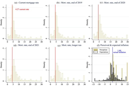
Distribution of pre-treatment perceptions and expectations of mortgage rate and inflation.
Notes: Mortgage rates are censored at 30%. Perceived inflation rate (point prediction) is censored at |$-$|10% and 15%. The blue vertical line shows actual inflation rate at the time of the survey. The red vertical line shows actual mortgage rate at the time of the survey. Expected inflation rate is based on the mean implied by the reported probability distribution for the 1-year-ahead inflation forecast.
Descriptive statistics.
| Robust moments | Moments | ||||
|---|---|---|---|---|---|
| Mean | Standard Deviation | Mean | Median | Standard Deviation | |
| (1) | (2) | (3) | (4) | (5) | |
| Pre-treatment data | |||||
| Perceived inflation, previous 12 months | 2.88 | 2.41 | 7.41 | 3.00 | 13.23 |
| Expected inflation, 12-month ahead | 2.32 | 2.02 | 3.62 | 2.60 | 3.69 |
| Perceived and expected mortgage rate for a “person like you” | |||||
| Current | 4.55 | 1.19 | 7.13 | 4.80 | 8.63 |
| End of 2019 | 4.90 | 1.44 | 7.59 | 5.00 | 8.74 |
| End of 2020 | 5.28 | 1.65 | 8.20 | 5.50 | 9.26 |
| End of 2021 | 5.53 | 1.92 | 8.74 | 6.00 | 10.07 |
| Next 5–10 years | 5.95 | 2.35 | 9.78 | 6.00 | 11.71 |
| Post-treatment data | |||||
| Expected inflation, 12-month ahead | 1.89 | 1.54 | 4.06 | 2.00 | 9.63 |
| Expected inflation, next 3–5 years | 2.42 | 1.79 | 4.65 | 3.00 | 9.47 |
| Perceived and expected mortgage rate for a “person with excellent credit” | |||||
| Current | 4.13 | 1.07 | 5.72 | 4.00 | 7.33 |
| End of 2019 | 4.39 | 1.09 | 6.02 | 4.50 | 6.96 |
| End of 2020 | 4.73 | 1.37 | 6.52 | 5.00 | 7.40 |
| End of 2021 | 4.97 | 1.57 | 6.88 | 5.00 | 7.83 |
| Next 5–10 years | 5.36 | 1.90 | 7.70 | 5.50 | 9.24 |
Notes: Pre-treatment expected inflation (12 months ahead) is computed as mean implied from the reported probability distribution over a range of bins. All other measures of inflation are reported as point predictions. Pre-treatment expected inflation excludes responses reporting deflation. Perceived and expected mortgage rates are elicited for “a person like you” at the pre-treatment stage and for “someone with excellent credit” at the post-treatment stage. Moments in columns (1) and (2) are computed using the Huber-robust method. The number of observations is 26,891.
The (robust) mean of perceived inflation over the 12 months preceding the survey is 2.88% (i.e. almost 1% point higher than the official inflation rate), in line with evidence from various consumer surveys according to which consumers tend to over-estimate recent inflation (see, e.g., D’Acunto et al. 2021a). The distribution of perceived inflation (Panel (a), Figure 2) shows a non-trivial fraction of respondents reporting focal values in excess of 10%, as in previous work (Binder 2017; D’Acunto et al. 2018a, 2019b).
To measure expected inflation, we use the probabilistic type of question asked in the SCE in which respondents are invited to assign probabilities over a range of inflation/deflation bins. However, the ordering of the inflation ranges presented in the survey began with deflation options before offering inflation ranges. This appears to have confused some respondents, who assigned all their weight to deflation outcomes but later provided positive answers to point forecast questions about inflation (even in the control group). To address this confounding factor, we drop expectations of inflation that have a negative implied mean from the distributional question (|$\approx$|20% of answers).7 Gorodnichenko and Sergeyev (2021) show that across a wide range of surveys and countries, the fraction of households expecting deflation is consistently under 1%. The discrepancy between all other household surveys studied in Gorodnichenko and Sergeyev (2021) and the large fraction of negative forecasts obtained in this setting is a clear indication that the ordering of bins confused some survey participants.8 Once we drop negative forecasts, the resulting expected inflation (12 months ahead) implied from the reported probability distribution is 2.3%. Comparable moments from the NY Fed’s SCE and Michigan Survey of Consumers were 2.8% and 2.9%, respectively, while professional forecasters were predicting CPI inflation of 2.3%. The consistency of the resulting mean forecasts in our survey after dropping deflationary expectations with the SCE and MSC provides another indication that the negative forecasts were mostly anomalous.
Moreover, the survey asks consumers about current and expected nominal interest rates with reference to a fixed rate 30-year mortgage. Mortgages with a 30-year fixed rate period represent the most popular mortgage product in the U.S., accounting for more than 70% of mortgages originated over the period 2013–2016.9 In our survey, respondents are asked to provide an estimate of the nominal interest rate for such a mortgage both at the time of the interview and over different time horizons (i.e. 1 year ahead; 2 years ahead; 3 years ahead; and in the next 5–10 years).10 The robust mean of the (perceived) current mortgage rate is 4.55% and the median is 4.80%. These moments are comparable with those derived from a similar question asked in the SCE (median: 4.3%; mean: 5.2%).11 Moreover, they are in line with Freddie Mac Primary Mortgage Market Survey, according to which the interest rate for a 30-year fixed rate mortgage was on average between 4.06% and 4.41% in March 2019.12 However, this masks significant heterogeneity in beliefs about interest rates. The robust standard deviation is 1.19%.13 Hence, for many households in the U.S., perceived market interest rates are quite far from actual interest rates. In the context of the Euler equation in Section 2, this means that |$i_t^{m}\ne i_t^{hh}$| for many households.
The expected mortgage rate 1 year ahead is 4.90% (i.e. 35 basis points higher, on average, than the perceived one at the time of the interview). As regards longer horizons, expected interest rates rise, on average, to 5.28%, 5.53%, and 5.95% with reference to 2 years ahead, 3 years ahead, and next 5–10 years, respectively. This implies that consumers expect somewhat higher mortgage rates in future periods. These trends are well aligned with the ones recorded in the SCE. Specifically, in the SCE the expected rate changes for 1 year ahead and 3 years ahead, compared with the current ones, are on average, 37 and 130 basis points respectively. Their counterparts in our survey are 35 and 98 basis points.
In Online Appendix Figure A.1 and Online Appendix Table A.1, we show various correlations between inflation expectations (1 year ahead) and other expectations asked in our survey. The raw data suggest a weak positive association between expected inflation and the expected mortgage interest rate 1 year ahead, yet considerable heterogeneity exists in this pattern. To this end, we examine not only how consumers respond to (exogenously) elevated inflation and nominal interest rate expectations but also to updates in the real rate expectations.
In short, our survey results for Nielsen panelists are consistent with those of other surveys of households. Average levels of perceived and expected inflation and interest rates are somewhat higher than actual levels and, strikingly, display large amounts of cross-sectional heterogeneity. Unlike other surveys, our results are based on a much larger cross-section of households (approximately 20,000 vs. 1,500 in the SCE and 500 in the MSC) and allow for randomized treatments that generate exogenous variation in beliefs within the same survey population and time period.
4. Econometric Framework
While estimating specification (1), we use sampling weights to correct for possible imbalances in the sample. Because expectations can take extreme values, we use Huber-robust regressions (1964) to minimize the adverse effects of influential observations and outliers. Huber-robust regressions differ from using winsorized data in standard regressions because they also take correlations across variables into account. Whether we include controls in specification (1) affects only the precision of the estimates because the assignment of treatment is random. To maximize statistical power and improve readability of our results, we estimate specification (1) with some treatments aggregated to coarser groups. We report detailed treatment effects in the Online Appendix.
Coefficient |$\alpha$| measures the persistence of expectations for the control group. Although one may naturally expect |$\alpha =1$| for post-treatment beliefs measured shortly after pre-treatment beliefs are elicited (the control group receives no information), the design of the survey as well as the nature of survey responses can result in estimates of |$\alpha$| different from one. First, pre- and post-treatment responses even in the control group can differ because respondents may have noise in their responses, leading to mean-reversion in answers. Second, as households participating in surveys do not like responding to the same question twice, we often formulate pre- and post-treatment questions differently. For example, we elicit inflation expectations before treatments by asking respondents to assign probabilities to a range of bins for possible inflation outcomes and use the reported probability distributions to compute the implied mean for expected inflation, whereas we gather the post-treatment inflation expectations as point predictions. Because responses often vary with the design of the survey questions (e.g. Bruine de Bruin et al. 2017), one may obtain |$\alpha \ne 1$|.16
Because survey responses can take implausible values, we drop some extreme observations. Specifically, for inflation forecasts, we drop responses of 100% or |$-$|100% for point predictions (drop 0.2% of the sample). We also drop observations with perceived/expected mortgage rates that are greater than 50% (drop less than 0.1% of the sample) and we censor mortgage rates at 30% if the responses are between 30% and 50% (applies to approximately 2% of the sample).
5. Effects of Different Information Treatments
In this section, we present and discuss how different treatments affect the expectations of individuals. To preserve space, we focus on the reaction of expectations immediately after the treatment and relegate results for beliefs in follow-up waves to the Online Appendix. In addition, we focus on estimates that pool across some different treatments to ease presentation but present full set of results for each treatment separately in Online Appendix Tables A.6–A.11.
5.1. The Effect of Forward Guidance Treatments on Interest Rate Beliefs
We begin by focusing on treatments regarding the future path of the federal funds rate relative to treatments focusing only on current and recent levels of the policy rate. Figure 3 first presents the cross-sectional relationship between prior and posterior beliefs for respondents receiving information about the Federal Funds Rate at different horizons. For each horizon, we present estimates pooled across treatments of the same horizon. Figure 4 (Panel (a)) presents how contemporaneous mortgage rate expectations of respondents then change when presented with information about different paths of the Federal Funds rate. For the control group that gets no information, the slope linking pre-treatment expectations to post-treatment expectations is close to 1 |${(\hat\alpha }=0.996$|, see Online Appendix Table A.9), indicating that measurement error in these expectations is quite small (as this would bias the estimated |$\alpha$| to values smaller than 1).17
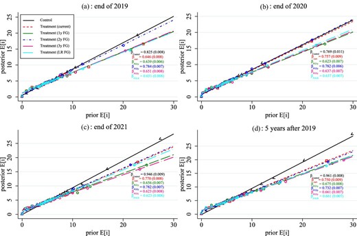
Response of nominal mortgage rate expectations by forecast horizon and the horizon of forward guidance (FG). Notes: Each panel shows binscatter plots for revisions in nominal mortgage rates when treatments are combined into information provision about current rates (“current”: T3, T19, and T24), 1-year forward guidance (“1y FG”: T7, T8, and T9), 2-year forward guidance (“2y FG”: T10, T11, and T12), 3-year forward guidance (“3y FG”: T13, T14, and T15), and longer-run forward guidance (“LR FG”: T4, T5, T6, T16, T17, and T18). The title of each panel indicates the horizon of the forecasts for mortgage rates. Estimated regression coefficients are reported in Online Appendix Table A.7.

Response of nominal mortgage rate expectations by treatment and horizon. Notes: Each panel shows binscatter plots for revisions in nominal mortgage rates when treatments are combined into information provision about current rates (“Current/past rates”: T3, T19, and T24), forward guidance (“FG”: T4–T19), and inflation (“Inflation”: T20–T23). The title of each panel indicates the horizon of the forecasts for mortgage rates. Estimated regression coefficients are reported in Online Appendix Table A.6. Panel A: by treatment type.
For those receiving information about only current and recent FFR (i.e. treatments 3 and 19), the slope of the relationship between priors and posteriors is flatter than the control group (approximately 0.8), as illustrated in Panel (a) of Figure 3. This indicates that telling households about current and recent levels of the policy rate has non-trivial effects on their beliefs about the current mortgage rate relative to their priors. Treatments that provide additional information about the path of the future FFR lead to indistinguishable effects on the perceived level of the current mortgage rate: treatments at the 1 year horizon (T7–T9), 2 year horizon (T10–T12), 3 year horizon (T13–T15), and longer horizon (T4–T6 and T16–T18) all lead to very similar slope relationships (|${\approx }$|0.8). Similar results hold for households’ beliefs about future mortgage rates (Panels (b)–(d)). Providing future estimates of the FFR leads to only small revisions in current perceptions of the mortgage rate, despite the fact that current information about the FFR is still included in the treatments. Similar results obtain for expected future mortgage rates, with few differences across treatments at longer horizons. A slope of 0.8 in the cross-sectional relationship between posteriors and priors implies that the average weight assigned to signals is only 0.2. We should therefore expect the response of households’ expectations of interest rates to be 20% of that of fully informed financial markets.
While the horizon of the guidance does not seem to have any effect on the degree to which households’ expectations respond, the level of interest rates in the guidance does. To see this, Table 3 reports the average revision in expectations about the nominal rate for treatments involving a high trajectory of interest rates (T4, T8, T11, T14, and T16), a medium trajectory (T6, T10, T13, and T18), or a low trajectory (T5, T9, T12, T15, and T17). Differences in the level of the signal should not affect the slope between posteriors and priors but only the intercept, which are captured by the average revisions in Table 3. We find that average revisions in beliefs about nominal interest rates, especially future ones, are generally smaller (more negative) for low trajectory treatments than high trajectory treatments, consistent with the level of the treatment affecting the average level of beliefs.
Response of expectations revisions by aggregated trajectory.
| Dependent variable: | Nominal mortgage rate | ||||
|---|---|---|---|---|---|
| revisions in perceptions or | Current | 1-year [2019] | 2-year [2020] | 3-year [2021] | Longer run |
| expectations of mortgage rate | (1) | (2) | (3) | (4) | (5) |
| Control | |$-$|0.191*** | |$-$|0.263*** | |$-$|0.330*** | |$-$|0.362*** | |$-$|0.358*** |
| (0.014) | (0.019) | (0.022) | (0.025) | (0.026) | |
| FG: high trajectory of FFR | |$-$|0.030* | |$-$|0.038* | |$-$|0.032 | |$-$|0.038 | 0.025 |
| (0.016) | (0.022) | (0.026) | (0.029) | (0.030) | |
| FG: central trajectory of FFR | |$-$|0.036** | |$-$|0.034 | |$-$|0.046* | |$-$|0.004 | |$-$|0.010 |
| (0.017) | (0.022) | (0.027) | (0.029) | (0.031) | |
| FG: low trajectory of FFR | |$-$|0.032** | |$-$|0.077*** | |$-$|0.072*** | |$-$|0.041 | |$-$|0.063** |
| (0.016) | (0.022) | (0.026) | (0.028) | (0.030) | |
| Current FFR rate | |$-$|0.042* | |$-$|0.051 | |$-$|0.099*** | |$-$|0.026 | |$-$|0.043 |
| (0.024) | (0.031) | (0.038) | (0.040) | (0.044) | |
| Current mortgage rate | 0.058** | 0.037 | 0.032 | |$-$|0.022 | 0.035 |
| (0.025) | (0.031) | (0.038) | (0.041) | (0.044) | |
| Inflation | |$-$|0.001 | |$-$|0.002 | |$-$|0.001 | 0.044 | 0.004 |
| (0.016) | (0.022) | (0.026) | (0.029) | (0.030) | |
| Observations | 19,425 | 19,909 | 20,313 | 20,370 | 20,247 |
| R-squared | 0.001 | 0.002 | 0.001 | 0.001 | 0.001 |
Notes: The table reports estimates of coefficients on treatment indicator variables when treatments are aggregated by the trajectory of forward guidance (FG) for the Federal Funds Rate (FFR). The estimated specification is |$X_j^{\textit {post}} - X_j^{\textit {pre}} = \alpha + \mathop \sum \nolimits _{k\ = \ 2}^{24} {\beta }_k {\textit Treatment}_j^{( k )} + {\textit {error}}_j$|. Coefficients for groups other than the control group are relative to the coefficient for the control group. All estimates are based on Huber-robust regressions. Regressions use sampling weights. No household/respondent controls are included. Robust standard errors are in parentheses.
Aggregation treatments: current FFR rate: T3; high trajectory: T4, T8, T10, T13, and T16; central trajectory: T6, T7, T11, and T14; low trajectory: T5, T9, T12, T15, and T17; current mortgage rate: T24; and inflation rate: T20–T23.*, **, and *** denote statistical significance at 10%, 5%, and 1% levels, respectively.
Because the signal is in terms of the policy rate while the expectations are in terms of the 30-year mortgage rate, the mapping between the two is not immediate. To get a sense of orders of magnitude involved, note that the average difference between the high and low interest rates in the treatments is approximately 70 basis points. From Figure 3, we see that treatments involving only the current rate affect future expected long-term interest rates almost as much as treatments involving future policy rates, suggesting that households view interest rates as quite persistent. Suppose this persistence is well-approximated by an autoregressive process of order 1 (AR(1)) with decay rate of |$\delta$|. The implied signal for the long-term rate that is equivalent to a 70 basis points persistent change in the FFR would then be approximately |$70/(30\times (1-\delta ))$| basis points. Typical Taylor rule estimates find a degree of interest smoothing of approximately 0.95 at the quarterly frequency, so |$\delta \approx 0.8$| at the annual frequency. Hence, this implies a comparable value of the signal in terms of the long-term rate of around 12 basis points. In other words, 12 basis points would be the expected change in the long-term rate in well-informed financial markets. But since households only put a weight of 20% on signals in updating their beliefs, we would expect the average revision in household beliefs arising from the different trajectories in interest rates to be around 2–3 basis points. Estimates in Table 3 are in this range, somewhat smaller for current nominal rates and slightly higher for future nominal rates, consistent with significant downweighing of the received signal on the part of households. While the specific path of the announced policy interest rate therefore does shape households’ long-term nominal interest expectations, the effect is significantly smaller than for financial markets due to the strong weight households place on their prior beliefs.
To summarize, we find that households’ interest rate expectations do not respond strongly to information about either past, current, or future policy interest rates. When presented with these treatments, households place a relative weight of around 80% on their prior beliefs, only one-fifth of the reaction that one might expect in financial markets.
5.2. Interest Rate Expectations after Other Treatments
How do households’ interest rate expectations respond to other types of treatments? Our experiment included two other types of information treatments that did not involve the policy rate. One alternative involved providing households with information about current or future inflation. Another involved providing households with direct information about the contemporaneous mortgage rate.
We illustrate how these different treatments affected households’ perceptions of nominal interest rates in Figure 4. For comparison, Panel (a) of Figure 4 plots the relationship between priors and posteriors over mortgage rates for information treatments involving current/past policy rates as well as information treatments involving forward guidance about policy rates. The effect of providing information about inflation (T20–T23) on perceived nominal rates is small. Posteriors for the current mortgage rate line up with priors in much the same way as for the control group. This result obtains whether we just include information about past inflation (T20–T21) or also include FOMC forecasts about future inflation (T22–T23). The latter in particular establishes that the FOMC predicts inflation to be very close to 2% in subsequent years, its longer-term inflation objective. The effects of inflation treatments have more impact on expectations of future interest rates (Panels (b)–(d)). For example, the effect on households’ expectations of mortgage rates at the end on 2021 is indistinguishable from when information about the policy rate is provided. This shows that information about inflation affects expectations of future interest rates, much as information treatments about interest rates also affect inflation expectations.
In contrast, the other information treatment involving the current mortgage rate (T24) has an immediate and very powerful effect on households’ perceptions of the current rate as well as their expectations of future mortgage rates. Panel (a) shows that posterior beliefs of households line up almost perfectly with the provided signal, regardless of respondents’ prior beliefs. The estimated slope of the relationship between posteriors and priors is 0.02. This effect holds not just for the contemporaneous mortgage rate (Panel (a)) but also for expectations over future levels of the mortgage rate (Panels (b)–(d)). Even for mortgage rates 2 years ahead, respondents place almost full weight on the signal about the current rate and effectively 0 weight on their prior beliefs.
By the standards of information treatments in macroeconomic RCTs, this level of convergence in reported beliefs toward the signal is, to the best of our knowledge, unprecedented. While it is not uncommon to find strong responses to information about variables that respondents are generally uncertain about, the full pass-through of the provided signal into reported beliefs, not just for the current mortgage rate but also for predicted mortgage rates years into the future, is very unusual. It suggests that providing information about the actual market interest rates that households face may be one of the more effective communication strategies available to central banks. The notion that communicating about targets, rather than instruments, can be most effective is consistent with the logic of Angeletos and Sastry (2021).
Taken together, we find that when presented with information about inflation, households do not revise their expectations about near term mortgage rates in an important way. In contrast, information about current mortgage rates—a market rate— has profound effects on households’ perceived and expected future mortgage rates.18
5.3. The Effects of Information Treatments on Inflation Expectations
As emphasized in Section 2, the effect of monetary policy communication on household consumption depends not only on how this communication affects the long-term nominal interest rates that households perceive but also their expectations about inflation. Indeed, some of the evidence from workhorse macroeconomic models described in Section 2 suggests that inflation expectations are the most important channel quantitatively. Because our survey includes questions about both nominal interest rate and inflation expectations, we are therefore able to assess the way that information treatments affect both sets of expectations, and therefore the real interest rates that households perceive.
Panel (a) of Figure 5 presents the effects of information treatments about different variables on inflation expectations, while Panel (b) of Figure 5 shows how the nominal interest rate information treatments affect expectations of inflation depending on the horizon of the information in the treatments. Several striking results arise with treatment-specific effects reported in Online Appendix Table A.10. First, information treatments involving recent and past inflation have very large effects on households’ inflation expectations, consistent with prior evidence in Coibion, Gorodnichenko, and Weber (2022). Second, information treatments involving current, past, and future levels of the policy rate have an effect on inflation expectations that is about as strong as treatments focusing directly on inflation. The implied weight on prior beliefs is only about 10%–20%. Importantly, this is not driven by a simple anchoring effect reflecting low numbers reported in the treatments: The placebo treatment of 2% population growth has only a small effect on expectations relative to the control group. The fact that information about policy rates affects inflation expectations could reflect an “information effect” in forward guidance: Lower future interest rates do not signal that monetary policy will be more accommodative (since this would be associated with higher expectations of inflation) but rather that the low interest rates will be a response to weaker inflationary pressures (hence, the simultaneous reduction in inflation expectations). This type of information effect has similarly been documented for professional forecasters in Nakamura and Steinsson (2018).
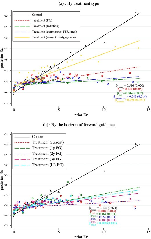
Response of inflation expectations by treatment type and by the horizon of forward guidance. Notes: Panel (a) shows binscatter plots for revisions in inflation forecasts when treatments are combined into forward guidance (T4–T19), inflation (T20–T23), and current/past interest rates (T3 and T19), and current mortgage rate (curr.mort., T24). Panel (b) shows binscatter plots for revisions in inflation forecasts when treatments are combined into information provision about current rates (“current”: T3 and T19), 1-year forward guidance (“1y FG”: T7, T8, and T9), 2-year forward guidance (“2y FG”: T10, T11, and T12), 3-year forward guidance (“3y FG”: T13, T14, and T15), longer-run forward guidance (“LR FG”: T4, T5, T6, T16, T17, and T18), and current mortage rate (curr.mort., T24). Estimated regression coefficients are reported in Online Appendix Tables A.6 and A.7.
The final result emanating from Figure 5 is that the information treatment involving the current mortgage interest rate has very little effect on inflation expectations relative to the control group. This is strikingly different from the fact that information about the current policy rate has very large effects on inflation expectations. The latter result suggests the presence of powerful information effects when it comes to the FFR, whereas no such effects appear to be present with the mortgage rate. Households therefore distinguish between the information content associated with different types of interest rates. This also suggests that policy communications may have very different effects on consumption depending on the type of interest rate discussed due to their differential effects on both inflation expectations and perceived nominal rates.
Overall, we find that households’ inflation expectations, unlike their interest rate expectations, respond quite strongly to information about current, past, or future policy rates. However, information about mortgage rates has little pass-through into inflation expectations.
5.4. The Effects of Information Treatments on Perceived Real Interest Rates
Economic theory predicts that, ultimately, the way in which information treatments affect consumption depends on the joint response of long-term interest rate perceptions and inflation expectations, that is, the response of households’ perceived real interest rates. This is not, in general, a simple combination of the responses of nominal interest rate expectations from Figures 3 and 4 with those of inflation expectations from Figure 5. To see this, consider the stylized effect of the inflation treatment: It leads to almost 0 revision in nominal interest rate perceptions but almost complete revision of inflation expectations toward the signal. One might think this would imply real interest rates would also necessarily converge as inflation expectations converge. However, if prior beliefs about nominal interest rates and inflation expectations are sufficiently positively correlated, the reverse could be true. In that case, someone with initially high inflation expectations (and who would therefore revise those expectations down sharply with the inflation treatment) would also be someone with high nominal interest rate expectations and therefore high real interest rate expectations (if the covariance between the two is sufficiently high). As that individual revises her inflation expectations downward, her real interest rate beliefs would rise and therefore deviate even more from the average. The inflation treatment could simultaneously lead to convergence in inflation expectations but divergence in real interest rate expectations depending on the joint distribution of beliefs about interest rates and inflation. This implies that it is important to consider the revision of beliefs jointly over nominal interest rates and inflation, that is, the revision in perceived real interest rates.
To do so, we define a household’s perceived real interest rate as their belief about the 30-year mortgage rate at the end of 2019 (it takes time to utilize interest rates) minus their expected rate of inflation over the next 12 months. Figure 6 then plots the posterior real interest rates perceived by households against their prior perceptions of the real rate, broken down by treatment type (Panel (a)) and treatment horizon (Panel (b)). Several results stand out. First, there is little difference in how households revise their views about the real interest rate across forward guidance treatments, current FFR treatments or inflation treatments. The slopes are approximately equal across treatments and are about 40%–60% of that of the control group. This reflects the fact that these treatments all affect perceptions of nominal interest rates and inflation in broadly similar ways, as well as the fact that prior beliefs about nominal interest rates and inflation are only weakly positively correlated in the pre-treatment data. Second, there are also few differences across treatment horizons, that is, whether information about rates is restricted to current and recent policy rates or whether they also provide information about the future path of interest rates. Third, we find that the mortgage rate treatment leads to larger revisions in perceptions of real interest rates: The slope of the relationship between priors and posteriors is about half as steep as for the other treatments. The implied relative weight on households’ prior beliefs about real interest rates is only about 10%.
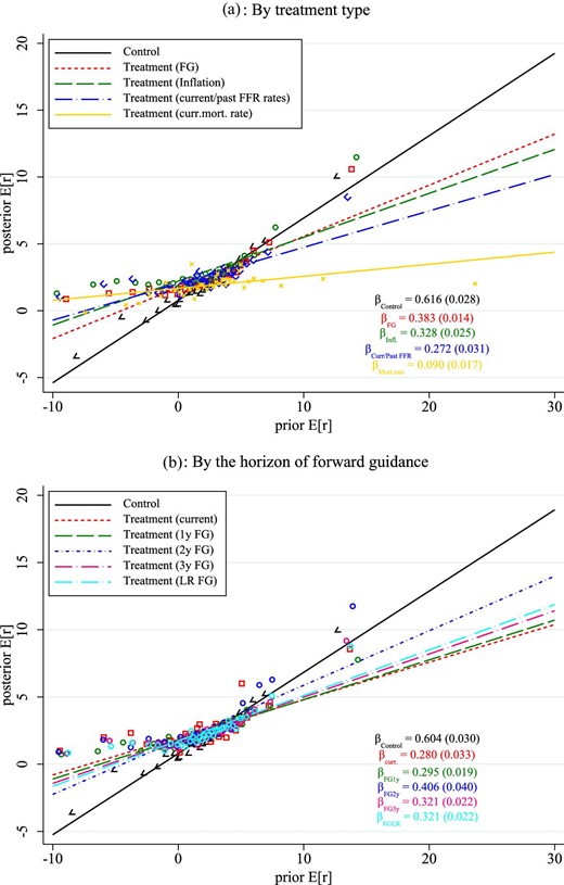
Response of real mortgage rate expectations by forecast horizon and the horizon of forward guidance (FG). Notes: Real rate is the mortgage rate in the end of 2019 minus the current 1-year-ahead inflation rate. Panel (a) shows binscatter plots for revisions in real mortgage rates (nominal mortgage rate minus 1-year-ahead inflation forecast) when treatments are combined into information provision about current FFR rates (“current”: T3 and T19), 1-year forward guidance (“1y FG”: T7–T9), 2-year forward guidance (“2y FG”: T10–T12), 3-year forward guidance (“3y FG”: T13–T15), longer-run forward guidance (“LR FG”: T4–T6 and T16–T18), and current mortgage rate (curr.mort., T24). Estimated regression coefficients are reported in Online Appendix Table A.7. Panel (b) shows binscatter plots for revisions in real mortgage rates (nominal mortgage rate minus 1-year-ahead inflation forecast) when treatments are combined into information provision about current FFR rates (“Current/past rates”: T3 and T19), forward guidance (“FG”: T4–T19), inflation (“Inflation”: T20–T23), and current mortgage rate (curr.mort., T24). The title of each panel indicates the horizon of the forecasts for mortgage rates. Estimated regression coefficients are reported in Online Appendix Table A.6.
As described in Section 2, the slope of the cross-sectional relationship between priors and posteriors speaks directly to how much weight agents place on new signals: A flat slope indicates a low weight on priors and therefore a large weight placed on new information. Successful communication by policymakers should target areas that households are most responsive to. Our results speak directly to this and suggest that providing information about the specific market interest rates faced by households is likely to be more powerful than communication strategies involving policy rates. However, both types of treatments are successful in leading households to revise their perceived real interest rates.
5.5. Persistence of Information Treatments
Previous research (e.g. Coibion, Gorodnichenko, and Weber 2022; Cavallo, Cruces, and Perez-Truglia 2017) documents that information treatments often have short-lived effects on households’ expectations. To assess the persistence of treatment effects in our survey, we compare posterior beliefs in two subsequent waves, performed 3 and 6 months after the initial treatment, to the prior beliefs of respondents.19 Results for perceived real interest rates are plotted in Figure 7. Consistent with prior work, we find that information treatments generally have transitory effects on beliefs. Most of the effects have dissipated 6 months after the treatment. The results are similar across treatments involving policy rates or inflation rates. However, the results with the mortgage rate treatment are again quite different. We find that effects on perceived real interest rates from the mortgage treatment are much more transitory than those from other treatments. Despite the very large contemporaneous effect of this treatment on households’ perceived real rates, the effects 3 months later are much smaller than those of the other treatments and have completely dissipated by 6 months. This suggests that communication about market interest rates, while potentially quite powerful in altering agents’ perceptions of real interest rates, are unlikely to have long-lived effects on those expectations.
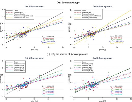
Response of real mortgage rate expectations by forecast horizon and the horizon of forward guidance (FG) in follow-up waves. Notes: The real rate is for the end of 2019. Panel (a) shows binscatter plots for revisions in real mortgage rates when treatments are combined into information provision about current FFR rates (“current”: T3 and T19), 1-year forward guidance (“1y FG”: T7–T9), 2-year forward guidance (“2y FG”: T10–T12), 3-year forward guidance (“3y FG”: T13–T15), longer-run forward guidance (“LR FG”: T4–T6 and T16–T18), and current mortgage rate (curr.mort., T24). Panel (b) shows binscatter plots for revisions in real mortgage rates when treatments are combined into information provision about current FFR rates (“Current/past rates”: T3 and T19), forward guidance (“FG”: T4–T19), and inflation (“Inflation”: T20–T23). The title of each panel indicates the horizon of the forecasts for mortgage rates.
5.6. The Effect of Real Interest Rates on Household Spending
Our results suggest that information treatments can have a strong effect on expectations of both nominal interest rates and inflation and therefore on perceived real interest rates. Economic theory predicts that changes in the latter, as illustrated in Section 2, should affect households’ consumption and saving decisions, thereby giving policymakers a powerful lever over the economy. Specifically, by varying the real interest rate, policymakers can influence consumption choices of households: An increase in the real interest rate should depress consumer spending contemporaneously.
To establish whether this prediction is borne out by the data, we construct measures of ex-post spending by households in the months following the information treatment. First, in the second follow-up wave 6 months after the treatment, households were asked whether they purchased a car, a house, or other large durable goods over the previous 6 months. This wave provides us with a self-reported measure of the extensive margin of durable goods purchases by households. Second, we can measure household spending on food and other available categories of goods tracked in the Nielsen Homescan panel over the 6 months following the survey. This source provides an external source of information on the purchases of select categories of non-durable goods by households. Third, both follow-up surveys asked households to report their spending over the previous months on a wide range of categories, allowing us to measure spending on food items (comparable to the Nielsen measure), all non-durable goods, and the sum of non-durable goods purchases and debt payments.
Estimating specification (2) with OLS is problematic because of mean-reversion in responses and other forms of endogeneity. Instead, we estimate specification (2) with an instrumental variables (IV) approach in which the first stage is given by specification (1).21 Effectively, this means that the revision in real interest rates is being instrumented by the information treatments, which are randomly assigned to some households and not to others. Coefficient |$\phi _1$| then yields a causal effect of changing expectations about real interest rates on ex-post household spending. The randomized provision of information helps us isolate exogenous variation in beliefs so that we can rule out endogenous co-movement in expectations and spending.22 As shown in Tables 4 and 5, our information treatments provide sufficient variation in perceived real rates for identification purposes.
The effect of real interest rates on the purchase of durable goods.
| Home | Car | Big item | Any | |
|---|---|---|---|---|
| (1) | (2) | (3) | (4) | |
| Posterior |$i - E\pi$| | |$-$|0.04 | |$-$|1.06** | |$-$|1.32*** | |$-$|1.33* |
| (0.10) | (0.41) | (0.41) | (0.72) | |
| [|$-$|0.217, 0.127] | [|$-$|1.746, |$-$|0.382] | [|$-$|1.995, |$-$|0.645] | [|$-$|2.525, |$-$|0.141] | |
| Plan to buy (pre-treatment) | 3.73*** | 7.39*** | 3.73*** | 8.64*** |
| (1.18) | (1.61) | (1.40) | (1.48) | |
| Prior |$i - E\pi$| | |$-$|0.01 | 0.23*** | 0.22*** | 0.20 |
| (0.02) | (0.08) | (0.07) | (0.13) | |
| Female | 0.46*** | 0.58 | 0.58 | 0.91 |
| (0.10) | (0.53) | (0.54) | (0.81) | |
| Age | |$-$|0.06 | |$-$|0.28* | |$-$|0.13 | |$-$|0.37* |
| (0.05) | (0.15) | (0.14) | (0.20) | |
| Age|$^{2}$| | 0.00 | 0.00* | 0.00 | 0.00* |
| (0.00) | (0.00) | (0.00) | (0.00) | |
| Have child | |$-$|0.05 | 1.18 | −0.81 | |$-$|0.11 |
| (0.33) | (1.05) | (0.95) | (1.54) | |
| HH head education: high school | |$-$|0.05 | 0.45 | |$-$|1.24 | |$-$|2.17 |
| (0.15) | (0.90) | (0.89) | (1.40) | |
| HH head education: some college | 0.06 | |$-$|0.83 | |$-$|1.03 | |$-$|2.95** |
| (0.15) | (0.76) | (0.82) | (1.27) | |
| HH head education: college or more | 0.54** | 0.13 | |$-$|0.77 | |$-$|1.56 |
| (0.23) | (0.87) | (0.81) | (1.35) | |
| ln(household income) | |$-$|0.00 | 0.01* | 0.00 | 0.01** |
| (0.00) | (0.00) | (0.00) | (0.00) | |
| Household size | 0.01 | |$-$|0.02 | 0.49* | 0.42 |
| (0.07) | (0.27) | (0.30) | (0.48) | |
| Observations | 5,784 | 5,779 | 5,780 | 5,738 |
| 1|$^{\rm st}$|-stage F-statistic | 9.99 | 10.41 | 9.14 | 10.17 |
Notes: The table reports IV estimates of specification (2). The first stage is given by specification (1). The dependent variable is equal to 100 if a respondent purchased a durable good of the type defined by each column (house in column (1), car in column (2), other big-ticket item in column (3), and any of these in column (4)) in the 6 months following the information treatment and 0, otherwise. All regressions use sampling weights. Robust standard errors are in parentheses. 90% confidence intervals robust to weak IV are reported in square parentheses. “1|$^{\rm st}$| stage F-statistic” reports the F-statistic for the first-stage regression. The treatment of outliers and influential observations is described in Online Appendix C of Coibion et al. (2019). 90% confidence interval robust to weak IV is reported in square parentheses. *, **, and *** denote statistical significance at 10%, 5%, and 1% levels, respectively.
The effect of real interest rates on non-durable goods spending.
| Wave | |||
|---|---|---|---|
| First follow-up | Second follow-up | Combined follow-up | |
| Panel A: Nielsen food | |||
| Posterior |$i - E\pi$| | 1.38 | 0.21 | 0.88 |
| (1.17) | (1.29) | (1.02) | |
| [|$-$|0.91, 3.67] | [|$-$|2.32, 2.74] | [|$-$|1.11, 2.88] | |
| Observations | 11,697 | 11,643 | 11,578 |
| F-statistic | 22.21 | 22.53 | 23.68 |
| Panel B: Nielsen total | |||
| Posterior |$i - E\pi$| | 2.93*** | |$-$|0.47 | 1.46 |
| (1.10) | (1.27) | (1.01) | |
| [0.78, 5.07] | [|$-$|2.96, 2.02] | [|$-$|0.51, 3.43] | |
| Observations | 11,653 | 11,574 | 11,527 |
| F-statistic | 22.50 | 22.58 | 23.90 |
| Panel C: survey food | |||
| Posterior |$i - E\pi$| | |$-$|0.32 | |$-$|0.09 | 0.67 |
| (2.28) | (3.13) | (2.27) | |
| [|$-$|4.79, 4.15] | [|$-$|6.73, 6.04] | [|$-$|3.78, 5.12] | |
| Observations | 10,751 | 5,418 | 4,588 |
| F-statistic | 14.59 | 6.734 | 6.792 |
| Panel D: survey non-durable | |||
| Posterior |$i - E\pi$| | 1.93 | |$-$|3.60 | |$-$|2.27 |
| (1.95) | (2.40) | (2.18) | |
| [|$-$|1.89, 5.76] | [|$-$|8.32, 1.11] | [|$-$|6.55, 2.01] | |
| Observations | 10,798 | 5,372 | 4,555 |
| F-statistic | 17.43 | 7.978 | 5.972 |
| Panel E: survey non-durable + debt payments | |||
| Posterior |$i - E\pi$| | 2.22 | |$-$|0.84 | 1.93 |
| (1.88) | (2.30) | (2.34) | |
| [|$-$|1.46, 5.91] | [-5.36, 3.67] | [|$-$|2.56, 6.53] | |
| Observations | 10,814 | 5,367 | 4,527 |
| F-statistic | 17.83 | 8.234 | 6.954 |
Notes: The table reports IV estimates of specification (2). The first stage is given by specification (1). The dependent variable is 100 |$\times$| log(monthly spending) over the last 3 months. Log(monthly spending) is trimmed at bottom and top 1%. Controls as in Table 4 are included but not reported. Panels A–E use different measures of spending. Panels A and B use scanner data from Nielsen. Panels C–E use self-reported spending data from the surveys. All regressions use sampling weights. Robust standard errors are in parentheses. 90% confidence intervals robust to weak IV are reported in square parentheses. “1|$^{\rm st}$| stage F-statistic” reports the F-statistic for the first-stage regression. The treatment of outliers and influential observations is described in Online Appendix C of Coibion et al. (2019). 90% confidence interval robust to weak IV is reported in square parentheses. *, **, and *** denote statistical significance at 10%, 5%, and 1% levels, respectively.
We report results for durable goods spending in Table 4 for each type of durable good separately and using all types of durable goods. For cars (column (2)) and big-ticket items (column (3)), we find that higher perceived real interest rates by households are followed by lower likelihoods of durable goods being purchased over the next 6 months. In the case of houses (column (1)), the coefficient is also negative but is not significantly different from zero, which likely reflects the fact that we have very few observations of house purchases over that 6-month period. When we combine all purchases of durables goods into one (column (4)), we again estimate a negative coefficient on real interest rates. Specifically, a 1% point decrease in the perceived real interest rate raises the probability of a large durable goods purchase in the next 6 months by around 1.1%–1.3% points, an economically strong response given that 7.1% of households reported buying a durable good over the last 6 months. Hence, exogenous changes in perceived real rates arising from our information treatments have a clear causal effect on subsequent household purchases of durable goods.23 This indicates that forward guidance, conditional on reaching households and changing their perceived real interest rates, can be expected to affect durable goods purchases of households within a relatively short time frame.
Results for non-durable goods purchases, 3 and 6 months after the information treatments, are reported in Table 5. We find little evidence of a robust response of non-durable goods spending to changes in perceived real interest rates. Regardless of whether we use narrow (food) or broad (all available spending) measures of spending from the survey or Nielsen, we find no statistically significant response of spending 6 months after the information treatments. Only with the Nielsen broad measure of spending over 3 months do we find a statistically significant effect, but it dissipates completely after another 3 months. Given that none of the other measures yield a similar result, we are inclined to treat it more as a noisy finding than clear evidence of a transitory change in non-durable goods spending. In all cases, the standard errors are quite large, which reflects the noisiness of non-durable goods spending data, whether it comes from scanners or is self-reported in surveys. In short, we view the results for non-durable goods spending as inconclusive: In contrast to interest-rate sensitive purchases of durable goods, we do not find evidence that changes in perceived real interest rates have discernible effects on ex-post household spending on non-durables, but the large standard errors also do not allow us to say that the effects are necessarily small.
6. Conclusion
Forward guidance is often thought to be a powerful tool to stimulate aggregate demand, especially when policy rates are constrained by the effective lower bound on nominal interest rates and large central bank balance sheets constrain further asset purchase programs. In typical theoretical models, forward guidance about future policy rates tends to lower the long-term interest rate perceived by households, which reduces the incentive to save and makes them willing to consume more, while raising their expectations about future price increases, which further encourages them to move their spending up. In more general settings, one would expect the effect on long-term nominal interest rates to happen via financial markets, so that consumers’ responses would ultimately depend on the extent to which they perceive those changes in market interest rates as well as the extent to which their inflation expectations respond to the announcement. This last channel is often the most quantitatively important in typical models. We contribute to this area by providing clear causal evidence of how information about current and future interest rates and inflation affects households’ expectations of both nominal mortgage rates and inflation.
Using a large-scale RCT on a representative sample of roughly 20,000 U.S. households, we find that communication about current and future policy rates moves both interest rate and inflation expectations by about as much as communicating about current or future inflation. These treatments are therefore successful in inducing households to revise their perceived and expected real interest rates. However, the pass-through is somewhat limited, as households continue to place a lot of weight on their prior beliefs (40%–60%). In contrast, communication about the mortgage rate has immediate and dramatic effects on household perceptions of these market interest rates, both current and those expected for years thereafter, while generating almost no offsetting changes in inflation expectations. The result is that real interest rate expectations end up being significantly more sensitive to the mortgage rate treatment than any other information treatment. We also document that lowering perceived real interest rates can stimulate spending on durable goods but it has no clear effect on spending on non-durables.
These results have a number of practical implications. One is that communication strategies could have much larger effects on household expectations and actions if they focused on objectives for long-term market interest rates, rather than policy rates, as emphasized in Angeletos and Sastry (2021). Second, we find the most effective communication strategies in terms of changing households’ expectations tend to be also the most transitory in their effects. Generating long-lived effects on expectations will require persistent communication campaigns.
The literature on the forward guidance puzzle has exclusively focused on trying to reduce the implied effects of forward guidance in theoretical models to conform to the empirical evidence of its effects. However, perhaps part of the puzzle comes instead from its implementation by policymakers: Alternative designs and strategies for forward guidance could yield much larger effects. With a better understanding of how to design forward guidance in a way that maximizes its effect on expectations, one might resolve the forward guidance puzzle in the opposite direction: by making its empirical effects rise to the levels predicted by standard theory.
Acknowledgments
We thank the Fama-Miller Center and the Initiative on Global Markets, both at The University of Chicago Booth School of Business, for financial support for conducting the surveys. Coibion, Gorodnichenko, and Weber also thank the NSF for financial support. We are grateful to Narayana Kocherlakota and seminar and conference participants at many institutions. We thank Jonas Dalmazzo, Mathieu Pedemonte, and Vitalia Yaremko for excellent research assistance. We also thank Shannon Hazlett and Victoria Stevens at Nielsen for their assistance with the collection of the PanelViews Survey. This research was funded in part by a grant from the National Science Foundation (#1919307). Results in this article are calculated based on data from The Nielsen Company (US), LLC and marketing databases provided by the Kilts Center for Marketing Data Center at The University of Chicago Booth School of Business. Information on availability and access to the data is available at http://research.chicagobooth.edu/nielsen. The randomized control trial is registered at the AER RCT Registry (#AEARCTR-0005378). The views expressed in this paper are those of the authors and do not necessarily reflect the views of the European Central Bank or of the Eurosystem. Coibion, Gorodnichenko, and Weber are affiliated at NBER.
Notes
The editor in charge of this paper was Guido Lorenzoni.
Footnotes
This line of work is not limited to the U.S. For example, Galashin et al. (2020) combine an RCT and credit card data for approximately 3,000 respondents in Malaysia. Apart from having a much larger sample, our study is different from Galashin et al. (2020) along other dimensions. For example, our study has a control group, applies different treatments (interest rates at different horizons rather than inflation and/or exchange rate), and has potentially more comprehensive measures of consumer spending (we use survey responses and scanner data).
Other channels of forward guidance on household consumption could operate independently of expectations effects. For example, changes in asset prices could lead to wealth effects on consumption. Changes in interest rates could also affect mortgage payments on adjustable rate mortgages, again allowing households to change consumption.
For example, Online Appendix Table A.6 reports estimates underlying Figures 4–6, which visualize key results of the paper. Online Appendix Table A.20 reports the corresponding p-values and p-values adjusted for multiple hypothesis testing where the latter are computed using the method developed in Anderson (2008). Both types of p-values are less than 0.1 % for nearly all coefficients.
We find no evidence that treatments can predict which respondents are dropped at this stage (Online Appendix Table A.21) and hence, our estimated treatment effects are not affected.
Treatment status does not predict which observations are dropped.
According to data from the National Mortgage Database program, jointly managed by the Federal Housing Finance Agency (FHFA) and the Consumer Financial Protection Bureau (CFPB).
Prior to our information treatments we ask respondents to give their estimates of the current and future (over different horizons) “interest rates on a fixed rate 30-year mortgage for someone like you”. To avoid repeating the same wording post-treatment, we ask this question with reference to “someone with excellent credit score”. Not surprisingly, reported interest rates to the latter question are somewhat lower to the pre-treatment ones, however they are not statistically different if one compares them for the control group.
In February 2019, the SCE asked the following question: “Assume that you applied for a 30-year fixed rate mortgage today. What mortgage rate do you think you would qualify for?” (source: https://www.newyorkfed.org/medialibrary/interactives/sce/sce/downloads/data/frbny_sce_housing_chartpacket2019.pdf).
The survey is conducted over mortgage lenders originating loans in the U.S. See FRED, Federal Reserve Bank of St. Louis; https://fred.stlouisfed.org/series/MORTGAGE30US.
For comparison, Bhutta, Fuster, and Hizmo (2020) report that the standard deviation of mortgage rates paid by U.S. households is approximately 0.5%.
Individual characteristics are gender, age, age squared, employed/unemployed/out-of-labor-force indicator, and race. Household characteristics are household income (binned; indicator variable for each bin), household size (indicator variable for each size), census region (indicator variable for each region), male head education (indicator variable for each group), and female head education (indicator variable for each group).
Intuitively, the posterior belief is a weighted average of the prior belief and the signal where the weight on the signal is equal to the gain of the Kalman filter and the weight on the prior is equal to 1 minus the Kalman gain. If the signal is not informative (or not available), then the weight on the prior is equal to 1. (Hence, |${\alpha =1}$| in specification (1).) If the signal is informative, then |$\gamma$| in specification (1) is equal to the negative Kalman gain. Coefficient |$\beta$| estimate the product of the signal and 1 minus the Kalman gain. See Coibion, Gorodnichenko, and Kumar (2018) for further discussion.
Another approach is to impose |$\alpha =1$| as was done in Galashin et al. (2020) who did not have a control group. Excluding the control group however presents a number of other challenges for estimating treatment effects (especially at the stage where we study the response of consumption to exogenous changes in expectations) and thus we do not take this route.
The placebo treatment (T2) “apprising respondents of the population growth over the last few years (approximately 2 % )’’ has an “anchoring” effect on mortgage rate expectations, but this effect is generally small.
We find little evidence that different types of individuals respond very differently from information treatments. For example, even comparing homeowners with outstanding mortgages to homeowners without debt or renters, information treatments have quite similar effects.
We find no systematic evidence of attrition across waves being related to the treatments (Online Appendix Table A.4).
To attenuate noise, we apply several filters to consumer spending on non-durables reported in the surveys and in the scanner data. For example, we exclude households who have inconsistent reporting in the scanner data. In a similar spirit, we exclude households who report unrealistically low or high consumer spending in the surveys.
To maximize statistical power, apart from a control group, we group treatments into: (i) future policy rates; (ii) past and current policy rates; (iii) inflation; and (iv) current mortgage rate.
To deal with outliers and influential observations, we adopt the jackknife procedure described in Coibion et al. (2019).
In Online Appendix Table A.19, we find equivalent results using as dependent variable whether households think that now is a good time to buy a durable good.
