


Abstract
We quantify the implications of voter bias and electoral competition for politicians’ gender composition. Unfavorable voters’ attitudes toward women and local gender earnings gap correlate negatively with the share of female candidates in Parliamentary elections. Using within-candidate variation across the different polling stations of an electoral district in a given election year, we find that female candidates obtain fewer votes in municipalities with higher gender earnings gaps. We show theoretically that when voters are biased against women, parties facing gender quotas select male candidates in the most contestable districts. We find empirical support for such a strategic party response to voter gender bias. Simulating our calibrated model confirms that competition significantly hinders the effectiveness of gender quotas.
1. Introduction
Despite significant progress in recent years, women are still largely under-represented among elected politicians, accounting for around 25% of Members of Parliament (MPs) across the world.1 While recent evidence suggests that female and male politicians tend to support different policy choices,2 there is no consensus on the key factors that drive the under-representation of women in politics. A large body of work has explored whether political parties favor male candidates (see, e.g., Norris and Lovenduski 1995), and recent studies have found mixed empirical evidence on the importance of party bias (Esteve-Volart and Bagues 2012; Casas-Arce and Saiz 2015; Bagues and Campa 2020, 2021). The possibility that women’s access to office might be restricted by voters’ preferences is also highly debated. The main reason for this is probably the difficulty of identifying voter bias in the data. Whether or not voter bias could account for the small share of women in politics therefore remains an open question (see the review in Krook 2018).3 Understanding the causes of women’s under-representation in politics has also important consequences for our knowledge of candidate selection and the quality of those who become politicians (Dal Bó et al. 2017).
In this paper, we quantify the role of voters’ preferences in the gender composition of politicians. We first show empirically that unfavorable voters’ attitudes toward women, measured either through survey data on gender role in politics or through local gender earnings gap, correlate negatively with the share of female candidates in French Parliamentary elections. Using within-candidate variation, we also find that female candidates obtain fewer votes in French municipalities with higher gender earnings gaps within an electoral district in the same election year. Our main theoretical and empirical contribution is then to show that electoral competition hurts women’s representation in politics when voters have a preference for male politicians, and when parties face gender quota on candidates. For this, we propose a model of political selection that sheds light on the trade-offs faced by political parties when policies encouraging gender diversity are introduced. We define as biased in favor of male politicians a voter who is more likely to vote for a male politician than for a female politician, when both politicians have the same ideology and expertise.4 We show that parties facing gender quotas on candidates select men rather than women in contestable districts (i.e., close races), if and only if voters are biased in favor of male candidates. We take this test to the French data and find strong empirical support for a strategic party response to voter bias in favor of male candidates. Finally, we calibrate the model, and show in simulations that electoral competition hinders the effectiveness of gender quotas in boosting women’s presence among elected politicians. The effect is quantitatively large: we find that an increase of 10% in the share of contestable districts reduces the increase in the fraction of elected women due to the introduction of gender quotas by around 25%.
A body of work in political science tests for the existence of a voter gender bias in survey experiments (e.g., Sanbonmatsu 2002; Schwarz, Hunt, and Coppock 2018; Teele, Kalla, and Rosenbluth 2018).5 In the first part of the paper, we follow an alternative strategy and measure the relation between voters’ attitudes toward gender in the field and gender gaps in the composition of candidates running for elections and in electoral outcomes.6 For this, we use both elicited data on gender roles in politics and administrative data on local gender earnings gaps—which for the latter allows us to proxy for differences in attitudes toward gender within the same electoral districts. In doing so, we rely on previous studies showing that (residualized) gender earnings gap reflects traditional or unfavourable views toward women’s role in society (Altonji and Blank 1999; Bertrand 2011).
We find that voters’ attitudes toward gender are strongly associated with the gender distribution of candidates across electoral districts within France, after controlling for a rich set of candidates’ characteristics, such as age, education, past occupation, and eventually political experience. A 10 percentage point increase in the share of respondents who agree with the statement “Men are better political leaders than women” is associated with a 2.3 percentage point decrease in the share of female candidates, a 10% drop from the sample mean. This result is robust to using respondents’ answers from the statement “When jobs are scarce, men should have more right to a job than women” or gender earnings gaps, as alternative proxies for voters’ attitudes. We then exploit the granularity of local gender earnings gaps in order to estimate the effect of voters’ attitudes on gender gaps in vote shares for the same female and male candidates, across municipalities of the same electoral districts in the same election.7 To the best of our knowledge, we provide the first granular analysis filtering out supply factors when estimating the effect of voters’ attitudes on electoral outcomes. We find a positive and strong correlation between gender earnings gaps and electoral gaps across municipalities: a one standard deviation increase in gender earnings gap leads to an increase by 0.6 percentage points in vote shares between male and female candidates. Overall, we find converging evidence that female candidates obtain lower votes in areas with less favorable attitudes toward women, and are less likely to run for elections in these areas.
We hypothesize that these two facts are linked and that parties refrain from selecting female candidates in districts with less favorable attitudes toward women because they anticipate a lower probability of winning elections when female candidates run in these districts. In the second part of the paper, we assess whether this strategic party response to the presence of voter bias accounts quantitatively for the low fraction of elected women, even after the introduction of gender quota on candidates. For this, we build a model of electoral competition (in majoritarian single-member constituency elections) in which political parties select candidates across districts taking into account that voters care about the gender of candidates in their districts. We first show that in the absence of gender quotas, parties always select the best candidate from each district—that is, the one who maximizes the probability of winning the election whatever the degree of political contestability. However, electoral competition shapes the selection of male versus female candidates in the presence of gender quotas on candidates. In that case, we show that parties strategically select men in contestable districts (i.e., close races) and women in non-contestable districts when voters are biased in favor of male candidates.
We take this prediction to the data and exploit the introduction in 2000 of gender quotas in French Parliamentary elections (referred to as the Parity Law), in which parties face fines when they deviate from a 50% national gender parity rule on candidates.8 We find strong empirical support for a strategic party behavior and the existence of a voter bias in favor of male candidates in French elections: while electoral competition has no effect on the gender allocation of candidates before 2000, we find that parties are more likely to select male candidates in contestable districts after the introduction of gender quotas.
Finally, we quantify the importance of voter bias and electoral competition in restricting women’s representation in politics. In our calibrated model, the fraction of female candidates pre-quota is 8%, in line with the data. When we introduce the parity rule in the model, we find that the electoral cost of selecting women when there is a voter bias in favor of male candidates outweighs the cost of the fine in the most contestable districts. This force is large enough for explaining why the main two parties select post-quota only 35% of female candidates, significantly below the objective of the Parity Law. We then conduct counterfactual simulations and confirm that an increase in competition would further significantly reduce the share of women elected in the Parliament.
Importantly, our results do not imply that intrinsic party bias—whereby political parties prefer male politicians per se—does not explain part of the low fraction of female politicians. Instead, we argue that voter gender bias generates a strategic party bias, which also matters quantitatively for understanding the under-representation of women in politics. To fix ideas, we propose an extension of our model that features both voter gender bias and intrinsic party bias in favor of male politicians. We show that parties with intrinsic preferences about politicians’ gender still refrain from selecting female candidates in the most contestable districts when facing gender quotas and voter gender bias. Simulation of this extension of the model confirms that electoral competition dampens significantly the effectiveness of gender quotas even in the presence of an intrinsic party bias.
This paper contributes to several strands of the literature. It first relates to a growing body of work on political competition and political selection. Prior empirical studies highlight the effect of political competition on accountability (Ferraz and Finan 2011), on the quality of politicians (De Paola and Scoppa 2011; Galasso and Nannicini 2011), on policy choices (Besley and Preston 2007; Stromberg 2008; Besley, Persson, and Sturm 2010), and on the transmission of political power within dynasties (Dal Bó et al. 2009). Folke and Rickne (2016) and Esteve-Volart and Bagues (2012) provide empirical evidence that electoral competition improves women’s position on the ballots of closed-list elections. We build on Galasso and Nannicini (2011)’s framework and provide the first formal model of electoral competition that incorporates voters’ preferences for politicians’ gender. We use the model to show that electoral competition harms women’s representation in French Parliamentary single-member district majority rule elections.9
We also contribute to the literature on the effect of gender quotas in politics,10 which is based on reduced-form evidence from several reforms. Gender quotas have been shown to affect the quality of politicians running for office (Baltrunaite et al. 2014; O’Brien and Rickne 2016; Besley et al. 2017), the type of policies implemented (Chattopadhyay and Duflo 2004; Baltrunaite et al. 2016), and beliefs about female leader effectiveness (Beaman et al. 2009; Paola et al. 2010). Another strand of the literature studies politicians’ incentives for voting in favor of the adoption of gender quotas. In that vein, Fréchette et al. (2008) propose as an explanation for the vote in favor of the 2000 Parity Law by the French Parliament a theory in which (male) incumbent politicians find it in their best interests to support the introduction of gender quotas when there is a voter bias in favor of male candidates: in doing so, they increase the probability of running against a woman and being reelected in the following election. Murray, Krook, and Opello (2012) offers an alternative view emphasizing the role of party pragmatism in passing the French Parity Law. Our study shifts the focus on the role of voter gender bias for understanding the consequences of gender quotas for parties’ political selection. Moreover, beyond reduced-form studies, our model allows us to conduct counterfactuals on the effect of gender quotas in boosting women’s representation among elected politicians depending on the degree of political competition.
More broadly, we also relate to the literature on the influence of social norms on economic and political outcomes. A few papers (Fernández, Fogli, and Olivetti 2004; Fortin 2005; Fernández and Fogli 2009; Alesina, Giuliano, and Nunn 2013) show how gender role attitudes influence gender gaps in labor market outcomes. In politics, Gagliarducci and Paserman (2012) find that the probability of early termination for elected female mayors in Italy is higher in regions with less favorable attitudes toward working women. Our finding that voters’ attitudes toward gender affect gender gaps in politics—both for differences in electoral scores and in the gender composition of candidates—has important consequences, and overall suggests that slow-moving voters’ attitudes might be an important factor that limits convergence toward a gender parity among politicians.
The remainder of this paper is organized as follows. In Section 2, we present French institutions and our data. In Section 3, we show how local differences in voters’ attitudes toward gender relate to the gender distribution of candidates across districts, and to gender gaps in electoral outcomes. We present our model of political selection with voter gender bias in Section 4, and take it to the data in Section 5. In Section 6, we run counterfactual simulations on the effect of gender quotas depending on the degree of political competition. Section 7 concludes.
2. Institutions and Data
2.1. French Institutions and Parliamentary Elections
The lower house of the French Parliament, the Assemblée Nationale, is composed of 577 members elected for 5 years (single-member constituencies), according to a two-round plurality voting rule.11 In every district, candidates compete in a first round. If no candidate obtains more than 50% of votes (and 25% of registered citizens), a runoff is set with candidates selected by more than 12.5% of registered citizens in round 1 (Pons and Tricaud 2018). The candidate with the most votes in the runoff wins the election. In practice, a vast majority of runoffs occur between two candidates, often with one candidate from the Right and one candidate from the Left.
We gather data for the last seven Parliamentary elections: 1988, 1993, 1997, 2002, 2007, 2012, and 2017.12 Our main empirical analysis focuses on candidates from the two main party coalitions: the Left coalition and the Right coalition.13 These two coalitions account for around 80% of elected MPs over the sample period.14 Their candidates have on average an ex-ante probability of being elected equal to 43%. By contrast, candidates from other parties have on average very low chances of winning a seat in the Parliament (i.e., around 1.5% in our sample).15 Given our focus on parties’ selection of candidates in a context of electoral competition, we exclude the other parties from our sample.
Figure 1 presents the share of female candidates in French Parliamentary elections over the last three decades. The share of female candidates hovers around 10% in the 1980s and 1990s, then almost doubles between the 1990s’ and the 2000s’ elections, and ranges between 35% and 40% in the last two elections in 2012 and 2017. This increase (at least partially) follows the introduction of gender quotas on candidates in French Parliamentary elections with the vote of the Parity Law in 2000, which we describe below.
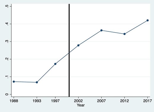
Fraction of women among candidates to French Parliamentary elections. The sample covers all candidates running for the two main Left and Right party coalitions.
The 2000 Parity Law
The Parity Law voted in 2000 stipulates that each party should have an equal fraction of male and female candidates across electoral districts in Parliamentary elections. When the difference between female and male candidates exceeds 4% (below 48% or above 52%), non-compliance with the 50% parity rule results in a financial penalty computed as follows: public funding provided to political parties based on the number of votes they receive in the first round of elections is reduced “by a percentage equivalent to one half of the difference between the total number of candidates of each sex, out of the total number of candidates”.16 As discussed in more details below, the 2000 Parity Law in French Parliamentary elections provides us with a unique laboratory for testing the presence of voter gender bias.
2.2. Data Sources and Variables
We use data from several sources: (i) administrative and web data on candidates and electoral outcomes; (ii) survey data on voters’ attitude toward gender; and (iii) administrative and census data on earnings and voters’ demographics across municipalities and electoral districts.
It is crucial for the analysis presented below to (at least) observe the gender of candidates, their party affiliation, as well as granular information on their electoral scores. We also gather data on other candidates’ characteristics that we use as control variables in the regressions presented below, such as age, education, occupation, and past political experience.
Candidates and Electoral Outcomes
The French Ministry of Interior has been publishing vote shares for each candidate, along with their gender and party affiliation, for Parliamentary (and Presidential) elections (at the electoral district level) since 1988.17 Vote shares are also available at the municipality level (within electoral districts) starting in 1993. The Ministry of Interior has also been providing information on candidates’ date of birth and occupation since 2012. We fill in missing information on date of birth and occupation in elections prior to 2012 using information from other sources.18 We then construct a dummy for high-skill occupations, such as managers, engineers, physicians, lawyers, and university professors.19 We also match candidates with the list of all members of government (from the fifth Republic starting in 1958), and we code whether candidates are alumni of an elite university, defined as graduates from the following list of French elite institutions: Ecole Polytechnique and Ecole Centrale Paris (for engineers), Ecole Nationale d’Administration (ENA, for public administration), Ecole des Hautes Études Commerciales (HEC, for business), and SciencesPo (for politicians).20 Finally, starting from the 2002 election, we construct a dummy for candidates with a local mandate, which equals 1 if the candidate has been elected as mayor or in the municipality council in the same electoral district where she/he runs for Parliamentary election.
We also rely on the timing of French elections—where Parliamentary elections are in the wake of Presidential elections since 2002—, and compute as a control for ideology/party popularity in each district the vote share that each party obtains in the previous Presidential election in the same electoral district. This also provides us with a measure of electoral contestability for each district. Specifically, we define as contestable districts for which the vote margin between the Left and the Right parties in the previous Presidential election was between −3 and +3 percentage points. We provide in Section 5 evidence on the predictive power of this measure. Importantly, this measure is gender-neutral as the Presidential candidates of the main parties are male, except in 2007 when Ségolène Royal ran from the Left party.
Proxies for Voters’ Attitudes
Our empirical analysis exploits the sizeable geographical differences in attitudes toward women across areas in France. Specifically, the analysis presented below relies on the Generation Gender Surveys (GGSs) that compile individual-level surveys on a variety of topics, including attitudes and preferences on gender roles in politics and in labor markets. The French wave of the GGS surveyed around 10,000 households in 2006. The survey is designed to be well-distributed geographically.
We follow Alesina, Giuliano, and Nunn (2013) and examine two questions that quantify individuals’ attitudes about gender roles. Using the GGS, we construct the share of respondents at the département level (the finest geographical unit available in the GGS)21 who separately agree with the following two statements: “On the whole, men are better political leaders than women” and “When jobs are scarce, men should have more right to a job than women”. The respondents are asked to choose among “strongly agree”, “agree”, “disagree”, “strongly disagree”, and “neither agree nor disagree”. As in Alesina, Giuliano, and Nunn (2013), we omit observations for which the respondents answered “neither agree nor disagree”, and compute for each département the average of respondents that answered “agree” or “strongly agree”.22
Unfortunately, this measure does not provide us with cross-sectional variation in voters’ attitudes toward gender within electoral districts, which would allow us to estimate the effect of voters’ attitudes on electoral scores of male versus female candidates keeping constant the supply of candidates. For this, we compute local gender earnings gap from the French employment registers [Déclarations Annuelles des Données Sociales (DADS)] as an alternative—and more granular—proxy for voters’ attitudes. The data are based on a mandatory employer report of the gross yearly earnings of each employee subject to French payroll taxes, and include all employed individuals. For our main analysis, we compute residualized local earnings gaps in order to absorb differences across municipalities related to local distributions of workers’ age and occupation, and of employers’ industry. In doing so, we rely on a large body of literature showing that residualized gender earnings gap reflects attitudes toward gender in labor markets (Altonji and Blank 1999; Bertrand 2011), and more generally on the role of women in society. However, differential selection into occupation by gender may also reflect gender attitudes. Therefore, we will also assess below the robustness of our results when using raw gender earnings gap.
We average gender earnings gaps either at the municipality level or at the broader electoral district level, in the year preceding each Parliamentary election.23
Summary Statistics
Table 1 presents summary statistics of our main sample, which consists of 7,038 candidate × election observations spanning seven Parliamentary elections in France from 1988 to 2017. We also present in Online Appendix Table A.1 the mean and standard deviation of the variables separately for male and female candidates.
Summary statistics—French Parliamentary elections.
| Observations | Mean | SD | p1 | p50 | p99 | |
|---|---|---|---|---|---|---|
| Panel A: candidates characteristics | ||||||
| Female | 7,038 | 0.240 | 0.427 | 0.000 | 0.000 | 1.000 |
| Age | 6,376 | 51.508 | 9.937 | 28.000 | 52.000 | 73.000 |
| Elite university education | 7,038 | 0.134 | 0.341 | 0.000 | 0.000 | 1.000 |
| High-skill occupation | 6,084 | 0.530 | 0.499 | 0.000 | 1.000 | 1.000 |
| First-time candidate | 7,038 | 0.366 | 0.482 | 0.000 | 0.000 | 1.000 |
| Incumbent | 7,038 | 0.314 | 0.464 | 0.000 | 0.000 | 1.000 |
| Former government member | 7,038 | 0.080 | 0.272 | 0.000 | 0.000 | 1.000 |
| Local mandate (from 2002 election) | 3,880 | 0.623 | 0.485 | 0.000 | 1.000 | 1.000 |
| Panel B: elections characteristics | ||||||
| Vote share (round 1) | 7,038 | 0.301 | 0.125 | 0.032 | 0.302 | 0.587 |
| Candidate elected | 7,038 | 0.429 | 0.495 | 0.000 | 0.000 | 1.000 |
| Presidential party vote share | 7,038 | 0.237 | 0.084 | 0.048 | 0.229 | 0.436 |
| Contestable district | 7,038 | 0.290 | 0.454 | 0.000 | 0.000 | 1.000 |
| Panel C: voters’ attitudes | ||||||
| Men better political leaders: % agree | 6,989 | 0.167 | 0.058 | 0.000 | 0.172 | 0.312 |
| Men more right to a job: % agree | 6,989 | 0.278 | 0.088 | 0.123 | 0.278 | 0.481 |
| Gender earnings gap (residualized) | 7,038 | 0.125 | 0.043 | 0.016 | 0.128 | 0.224 |
Notes: This table presents the summary statistics for our sample, which consists of 7,038 candidate–district observations over seven Parliamentary elections between 1988 and 2017. There are 3,890 unique candidates in this sample. A candidate is included in the sample if she/he is running for the Left or Right coalition in a given election. Female is a dummy if the candidate is a woman. Age is the age of the candidate at the time of the election. Elite university education is a dummy for graduates of the following list of French elite institutions: Ecole Polytechnique, Ecole Centrale Paris, Ecole Nationale d’Administration, Ecole des Hautes Études Commerciales, and SciencesPo. High-skill occupation is a dummy indicating whether the candidate was either a manager, engineer, physician, lawyer, or university professor. First-time candidate is a dummy indicating whether the candidate is running in a Parliamentary election for the first time. Incumbent is a dummy if the candidate has been elected in the previous Parliamentary election in the same district. Former government member is a dummy indicating whether the candidate has been a member of a former government. Local mandate is a dummy indicating whether the candidate has been elected either as mayor or in the council of a municipality in the same Parliamentary district (available only from 2002). Vote share is the number of votes obtained by the candidate in the first round of a given Parliamentary election over the total number of votes in the same district and election. Candidate elected is a dummy for the candidate winning the election in the district. Presidential party vote share is the vote share obtained by the candidate’s party in the previous Presidential election. Contestable district is a dummy, which equals 1 if the vote margin between the Left and the Right parties in the runoff of the previous Presidential election was between −3 and +3 percentage points (respectively, in the first round of the previous Presidential election for the 2002 and 2017 Presidential elections). Men better political leaders: % agree and Men more right to a job: % agree are drawn from the 2006 GGS, and are computed at the département level. Gender gap in earnings is the average residualized gender gap (between men and women) in the district in the year preceding the election.
There are 24% of female candidates, and the average age of candidates is 52 years. A total of 13% are alumni from elite universities, and 53% worked in high-skill occupations. In terms of political experience, 37% of candidates run for the first time, 31% are incumbents in the same district, 8% of candidates were members of a former government (at the time of the election), and 62% hold a local mandate in the same district as where they run for Parliamentary election. We also check that candidates tend to run in the same district across elections: 96% of repeat candidates run in the same district.
Panel B presents electoral outcomes. While there are on average eleven candidates (from all parties) running for election in a given district, Left and Right candidates of the two main parties in our sample capture a disproportionally large fraction of the votes: their (individual) vote share is on average 30% in the first round of the election, and their overall probability of being elected is 43%. Using candidates’ parties’ vote shares in the previous Presidential election, we end up with 29% of electoral districts being classified as (ex-ante) contestable. As shown in Online Appendix Table A.1, female candidates obtain on average lower vote shares and are less likely to be elected in Parliamentary elections.
Panel C presents summary statistics for our measures of voters’ attitudes at the geographical level. What is relevant for our work is the cross-sectional variability of these measures, which is substantial for each of them. Importantly for our approach, we then show in Online Appendix Table A.2 that these measures are strongly correlated between them, both within survey respondents and across geographical areas. We find in columns 1 and 2 a strong and statistically significant correlation between attitudes toward gender in politics and on labor markets at the individual level, measured with respondents’ answers to the statements “On the whole, men are better political leaders than women” and “When jobs are scarce, men should have more right to a job than women” in the GGS. This correlation remains robust after aggregating answers at the département level, as shown in column 3. Finally, we relate earnings gaps with survey data in column 4, and find a large and statistically significant correlation between local gender earnings gaps and voters’ attitudes in the GGS: Namely, a one standard-deviation increase in local earnings gap accounts for 46% of the standard deviation in the local share of individuals who agree with the statement “On the whole, men are better political leaders than women”.
3. Voters’ Attitudes and Gender Electoral Gaps: Reduced-Form Evidence
In this section, we provide reduced-form evidence on the importance of voters’ attitudes for (i) the share of women candidates in French Parliamentary elections; and (ii) gender electoral gaps—defined as the difference in vote shares between male and female candidates. We measure geographical differences in voters’ attitudes using both survey data aggregated at the département level and local gender earnings gaps, either at the electoral district or at the municipal level. These measures are increasing with the degree of unfavorable attitudes toward women.
3.1. Voters’ Attitudes and Selection of Male/Female Candidates
Table 2 reports the estimates of our parameter of interest β separately for our three proxies for voters’ attitudes.24 In panel A, we proxy for unfavorable attitudes toward women with the share of agreement with the statement “Men are better political leaders than women”. The coefficient is negative, statistically significant, and stable across specifications. The effect is also economically significant: a 10 percentage point increase in the share of respondents considering that “Men are better political leaders than women” is associated with at least a 2.3 percentage point decrease in the probability that the candidate is a woman, a 10% decrease compared to the 24% sample mean of female candidates. The estimate hardly changes when we further control for candidates’ age, education, and previous occupation, in column (2), and for political experience in column (3). We control for political experience using dummies for incumbents, for candidates running for a Parliamentary election for the first time, for former members of government, and for holding a local mandate. Although these controls are potentially endogenous—for example, being the incumbent is a past outcome—, we find robust results. Finally, we further control in column (4) for the vote shares of candidates’ affiliated party obtained in the same electoral district during the previous Presidential election. The coefficient remains large and statistically significant.25
Voters’ attitudes and selection of male/female candidates.
| (1) | (2) | (3) | (4) | (5) | |
|---|---|---|---|---|---|
| Panel A: | Female candidate? | ||||
| Men better political leaders: % agree | −0.228* | −0.269** | −0.267** | −0.301*** | |
| (0.120) | (0.119) | (0.115) | (0.115) | ||
| Election × party fixed effects | Yes | Yes | Yes | Yes | |
| Age, education, occupation | No | Yes | Yes | Yes | |
| Incumbent, first run, government exp. | No | No | Yes | Yes | |
| Presidential party vote share | No | No | No | Yes | |
| District fixed effects | No | No | No | No | |
| Observations | 6,989 | 6,989 | 6,989 | 6,989 | |
| R2 | 0.127 | 0.163 | 0.208 | 0.211 | |
| Panel B: | Female candidate? | ||||
| Men more right to a job: % agree | −0.268*** | −0.290*** | −0.299*** | −0.332*** | |
| (0.076) | (0.076) | (0.072) | (0.071) | ||
| Election × party fixed effects | Yes | Yes | Yes | Yes | |
| Age, education, occupation | No | Yes | Yes | Yes | |
| Incumbent, first run, government exp. | No | No | Yes | Yes | |
| Presidential party vote share | No | No | No | Yes | |
| District fixed effects | No | No | No | No | |
| Observations | 6,989 | 6,989 | 6,989 | 6,989 | |
| R2 | 0.129 | 0.165 | 0.210 | 0.214 | |
| Panel C: | Female candidate? | ||||
| Gender earnings gap (district) | −0.473*** | −0.481*** | −0.494*** | −0.525*** | −0.647** |
| (0.158) | (0.159) | (0.152) | (0.152) | (0.273) | |
| Election × party fixed effects | Yes | Yes | Yes | Yes | Yes |
| Age, education, occupation | No | Yes | Yes | Yes | Yes |
| Incumbent, first run, government exp. | No | No | Yes | Yes | Yes |
| Presidential party vote share | No | No | No | Yes | Yes |
| District fixed effects | No | No | No | No | Yes |
| Observations | 7,038 | 7,038 | 7,038 | 7,038 | 7,038 |
| R2 | 0.128 | 0.164 | 0.209 | 0.212 | 0.344 |
Notes: This table presents estimates from regressions of candidates’ gender on the fraction of respondents in each département in the 2006 GGS who agree with the statement “Men are better political leaders than women” (panel A) and those who agree with the statement “When jobs are scarce, men should have more right to a job than women” (panel B) and on (residualized) gender earnings gaps (panel C). Regressions include election × party fixed effects. Columns (2)–(5) include dummies for candidates’ age, elite university education, and high-skill occupations. Columns (3)–(5) include dummies for incumbents, first-time candidates, and former government members, as additional controls. Columns (4) and (5) also control for the vote share obtained by the candidate’s party in the previous Presidential election. Column (5) includes district fixed effects (panel C only). The sample is restricted to candidates from the main Left and Right party coalitions. Regressions are at the candidate–district level over the Parliamentary elections between 1988 and 2017. Standard errors presented in parentheses are clustered at both the candidate and département levels in panels A and B and at both the candidate and district × election levels in panel C. *, **, and *** denote significance at the 10%, 5%, and 1% levels, respectively.
In panel B, we use the statement “When jobs are scarce, men should have more right to a job than women”, and find very similar results. If anything, the economic and statistical significances of the estimates are stronger.
Panel C reports the estimates of β when using gender earnings gaps as a proxy for voters’ attitudes, which varies both across electoral districts and over time.26 As for panels A and B, the coefficients are negative, statistically significant at conventional levels, and stable across specifications. The estimates are also economically large: a one standard deviation increase in the gender earnings gaps is associated with at least a 2 percentage point decrease in the probability that the candidate in that district is a woman. Note that we introduce district fixed effects in column (5), so that the coefficient is now identified through within-district variations in the gender earnings gap over time. We still obtain a large and negative coefficient.
Overall, we find converging evidence that female candidates are less likely to run for elections in areas with (relatively) unfavorable attitudes toward women. One explanation for this pattern—formalized in the model presented in Section 4—is that parties anticipate a lower probability of winning elections when female candidates run in districts with unfavorable attitudes toward women. However, one might think of alternative explanations, such as, for instance, the possibility that the local supply of female versus male candidates vary across districts with more or less favorable attitudes toward women.27 We thus directly test below whether female candidates indeed obtain lower votes in areas with less favorable attitudes toward women.
3.2. Voters’ Attitudes and Gender Gaps in Vote Shares
We will interpret a negative sign for the main parameter of interest β in equation (2) as supportive evidence that female candidates obtain lower votes in municipalities with higher gender earnings gaps. While reverse causality should not be a threat to our interpretation since the evidence comes from within-constituency comparison, which shuts down differential response by women candidates, one may still worry about omitted variable bias: (i) the possibility that what drives the correlation between earning gaps and female candidates’ vote shares is not really candidates’ gender but correlated candidate-level factors; and (ii) the possibility that what drives the correlation is not really the earnings gap but correlated municipality-level factors such as the sex ratio. We address below the first set of concerns with the inclusion of a series of candidates’ characteristics other than gender in interaction with earnings gaps in equation (2), the vector |${\textit{GenderEarningsGap}}_{m,t} \times X_{i,t}$|. We address the second set of concerns by introducing in augmented specifications the gender dummy interacted with a list of municipality-level confounders.
Table 3 reports estimates for our main parameter of interest β. The coefficient β on the interaction between gender earnings gaps and the dummy for female candidates is negative and statistically significant (at 1% confidence level) in all specifications: female candidates obtain on average lower vote shares compared to male candidates in municipalities in which the male–female earnings gap is larger. We gradually introduce candidate × election fixed effects and controls for candidates’ characteristics (dummies for elite education and for high-skill occupations, and previous political experience) in interaction with earnings gaps. Importantly, we introduce the party affiliation of the candidate interacted with earnings gaps in column (5). This controls for the concern that high gender earnings gap municipalities are more likely to vote for the Right party, of which women are less likely to be a member.29 Reassuringly, the β coefficient is still negative and statistically significant at the 1% confidence level. In column (6), we find that the coefficient β is similar for female candidates from the Left and the Right parties. This suggests that gender attitudes translate into the same gender electoral gaps whatever the ideology of voters.30
Voters’ attitudes and gender gaps in vote shares—-municipality level.
| (1) | (2) | (3) | (4) | (5) | (6) | |
|---|---|---|---|---|---|---|
| Vote share—round 1 | ||||||
| Female × gender earnings gap | −0.421*** | −0.364*** | −0.275*** | −0.197*** | −0.078** | |
| (0.055) | (0.039) | (0.036) | (0.035) | (0.033) | ||
| Female × Right party × gender earnings gap | −0.058 | |||||
| (0.046) | ||||||
| Female × Left party × gender earnings gap | −0.090** | |||||
| (0.041) | ||||||
| Female | −0.029*** | |||||
| (0.004) | ||||||
| Municipalities × election fixed effects | Yes | Yes | Yes | Yes | Yes | Yes |
| Candidate × election fixed effects | No | Yes | Yes | Yes | Yes | Yes |
| Age, education, occupation × earnings gap | No | No | Yes | Yes | Yes | Yes |
| Incumbent, first run, government exp., × earnings gap | No | No | No | Yes | Yes | Yes |
| Right party × earnings gap | No | No | No | No | Yes | Yes |
| Observations | 286,121 | 286,121 | 286,121 | 286,121 | 286,121 | 286,121 |
| R2 | 0.680 | 0.891 | 0.892 | 0.893 | 0.895 | 0.895 |
Notes: This table presents estimates from regressions of candidates’ vote shares in the first round of the Parliamentary elections on a female candidate dummy interacted with residualized gender earnings gap at the municipality level, and control variables. Earnings gaps are computed at the inter-municipality level for small municipalities (defined as those below 2,000 inhabitants). All regressions include municipality × election fixed effects. Columns (2)–(5) include candidate × election fixed effects. Some specifications include controls for the interaction between residualized gender earnings gap and other characteristics of candidates (age, elite university education, high-skill occupation, political experience, and party affiliation). The sample is restricted to candidates from the two main party coalitions. Regressions are at the candidate–municipality level over the Parliamentary elections from 1993 to 2017. Standard errors presented in parentheses are clustered at both the candidate and municipality–election levels, and regressions are weighted by total population in each municipality. *, **, and *** denote significance at the 10%, 5%, and 1% levels, respectively.
Taking column (5) as our preferred specification, we obtain that a one standard deviation in gender earnings gap (7.2 percentage points at the municipality level) is associated with a decrease by 0.6 percentage points (0.072 * 0.078) in the vote share of female candidates (relative to male candidates).31 For means of comparison, note that in our sample, there are around 12% of tight outcomes in the second round of the Parliamentary elections with vote margins between the two candidates within ±1% (in which case a difference of 1 percentage points would change the outcome of the election). This confirms that voters’ attitudes matter quantitatively for electoral outcomes between male and female candidates.32
Robustness
In Robustness checks presented in Online Appendix Table A.3, we take our specification in column (5) of Table 3 and add the gender dummy interacted with other municipality characteristics (that could arguably confound the effect of voters’ attitudes on gender electoral gaps documented in Table 3). For example, one potential concern is that male voters could tend to prefer male candidates, while female voters tend to prefer female candidates. If gender earnings gaps are correlated with sex ratios across municipalities, this could confound the interpretation of our coefficient of interest. Instead, we find in column (1) of Online Appendix Table A.3 that the estimate on the interaction term between earnings gap and the female candidate dummy is unchanged when we control for the interaction of the sex ratio and the female candidate dummy. More generally, Online Appendix Table A.3 shows that our coefficient of interest is unaffected when we further interact the female candidate dummy with total population in the municipality, the overall employment rate, or the share of men among employed workers.
One remaining concern that is not fully addressed by our within-candidate framework is that women running for elections would be more likely to live or come from municipalities with more favorable gender attitudes, and could obtain more votes in these municipalities because of their local roots. To tackle this concern, we run the same regression as above in which we add a dummy for whether candidate i has been either council member or the mayor in municipality j. If the larger fraction of votes obtained by female candidates in municipalities with low gender earnings gap simply reflects a “home bias”, including this control would arguably absorb part of the main coefficient of interest Female × Gender Earnings Gaps. We present the results in Online Appendix Table A.4. First, we do find strong evidence that candidates with a local mandate in a given municipality obtain larger vote shares when running for Parliamentary election. However, including the control for local mandate has virtually no effect on the coefficient of interest Female × Gender Earnings Gaps. This largely mitigates the residual concern that selection into politics within districts could explain our findings.
One econometric concern is that gender earnings gaps are not precisely estimated in small municipalities. While Table 3 includes all municipalities, we show in Online Appendix Table A.5 that the results are robust in unweighted regressions restricted to municipalities with more than 2,000 inhabitants.33 Finally, we show in Online Appendix Table A.6 that the results are robust to using gender gaps in raw earnings or in earnings residualized with fewer controls.
Overall, we interpret the results presented in Tables 2–3 as evidence that voters’ attitudes toward women matter quantitatively for understanding gender differences in both selection into politics and electoral outcomes. We use these stylized facts as a motivation for building a model of electoral competition in which parties select candidates taking into account that voters might have a systematic preference for either male or female candidates, referred to as “gender voter bias” in what follows.
4. Model of Electoral Competition
We aim at modeling electoral competition in single-member district majoritarian elections with two main parties.34 We build on Galasso and Nannicini (2011) and propose a model of political selection in which parties choose between candidates that differ in terms of valence and gender in order to win elections. Our theoretical innovation is to add gender as an additional source of heterogeneity across candidates along with a potential voter gender bias (which then makes gender an important attribute of candidates in the model).
The model provides new insights into how voter gender bias and gender quotas affect political selection, and ultimately the gender composition of elected politicians. Specifically, the main contribution of the model is to provide a theory in which the political under-representation of women is partly explained by parties’ strategic response to voters’ bias. We show that the presence of voter gender bias endogenously generates a strategic party bias in the presence of gender quotas, that is, parties refrain from selecting female (respectively, male) candidates in the most contestable districts when voters have a preference for male (respectively, female) candidates. This insight serves as a model-based test for the presence (and sign) of voter bias that we bring to the data in Section 5. We present an extension of the model with intrinsic party bias in Online Appendix C that highlights the robustness of our model-based test for the presence of voter gender bias. The second contribution of the model, which we develop in Section 6, is to show how parties’ strategic decisions alter the effectiveness of gender quotas in the presence of electoral competition.
4.1. Setup
We consider two main parties: Left and Right (denoted L and R below), and k = 1, …, N electoral districts. The two parties occupy fixed positions in the ideology profile: IL = −1 and IR = 1. They compete under a single-member district majority rule. The elected candidate provides support for her/his ideology and constituency services for her/his district. Each potential candidate has a personal valence that can be understood as a combination of her/his education, oral ability, political experience, and effort at work. Districts vary by their local ideology, so that some are contestable, while in others the candidate of one party (either L or R) is ex-ante likely to win the seat.
Parties and Districts
Candidates
In each district, party R (respectively, L) chooses between two local candidates—a female candidate and a male candidate—with valence |$\theta ^F_{R,k}$| and |$\theta ^M_{R,k}$| (respectively, |$\theta ^F_{L,k}$| and |$\theta ^M_{L,k}$|).36 The assumption that parties select candidates among a pool of local candidates, as opposed to allocating a national pool of candidates across electoral districts, is consistent with the data. We find that 80% of candidates either hold (or used to hold) a local mandate in the council of one municipality of the same district and/or run in the same district for parliamentary election in one of the previous elections.37 We assume that female and male candidates’ valences are drawn from the same uniform distribution |$\mathcal {U}[-\bar{\theta }, \bar{\theta }]$|.38 The valence of each candidate is common knowledge.
Voters and Electoral Competition
|Ik − IL| − |Ik − IR| + θR,k − θL,k − bFR,k + bFL,k can be interpreted as an ex-ante score of party R in district k (i.e., before the realization of the campaign electoral shock δk). Φ( · ) maps ex-ante score into expected probability of winning the election in a given district.
Timing
We adopt the following timing for the electoral game that the two parties play in each district k: (stage 1) nature draws the local ideology Ik, the potential candidates’ valences |$\lbrace \theta _{R,k}^F,\theta _{R,k}^M,\theta _{L,k}^F,\theta _{L,k}^M\rbrace$|, and which party chooses its local candidate first (say L in what follows); (stage 2) party L chooses its candidate in {FL,k,ML,k}; (stage 3) party R chooses its candidate in {FR,k,MR,k}; and (stage 4) nature draws the campaign popularity shock δk, voters vote, and one candidate is elected.
We assume that the probability of moving first is the same for both parties.43 All nature draws are common knowledge.
Equilibrium
We solve for a subgame perfect equilibrium. The equilibrium in each district k is the gender pair of the Left and Right candidates (FL,k,FR,k) [either (0,0), (1,1), (0,1), or (1,0)] and it depends on the parameters |$\lbrace c,b,I_k,\theta ^F_{R,k},\theta ^M_{R,k},\theta ^F_{L,k},\theta ^M_{R,k}\rbrace$|. We formally solve for the equilibrium of the game for all parameter values in Online Appendix B. In the next section, we give the main intuition for political parties’ best responses in the selection of female or male candidates in each district.
4.2. Parties’ Selection of Candidates
The main intuition, described in this section, is that the decision of selecting a female versus a male candidate depends in particular on the difference in valence between the two candidates, the degree of voter bias, and the degree of political competition in the district when there is a cost (c > 0) of deviating from the gender parity rule on candidates. To begin with, we describe parties’ selection of male or female candidates across electoral districts for the case c = 0 (without costs for deviating from the parity rule on candidates).
Pre-Quota Environment Benchmark (c = 0)
In the absence of gender quotas (c = 0), parties’ objective (see equation (3)) boils down to maximizing VR,k, the probability of winning the election in each district. It follows that in each district, each party selects from between the male and female candidates the one with the best chance of winning. That is, party R (the same applies to L) chooses the female candidate if and only if |$\theta _{R,k}^F-b>\theta _{R,k}^M$|, and the male candidate otherwise. The following lemma summarizes the selection of candidates and characterizes the aggregate gender composition of candidates when c = 0. The proof is in Online Appendix B.
In the absence of gender quotas (c = 0), in each district k, party R (the same applies to L) selects the female candidate if |$\theta _{R,k}^{F}-\theta _{R,k}^{M} \ge b$|, and the male candidate otherwise.
The voter gender bias, b, affects the aggregate fraction of male versus female candidates. When voters have a preference for male politicians (b > 0), parties select female candidates only when their valence is large enough to compensate for the degree of voter bias. Aggregating over the (uniform) distribution of valence, the share of female candidates is |$1/2-b/(2\bar{\theta })$|. That is, the share of female candidates running for election is exactly 50% in the absence of voter bias, and below 50% (respectively, above 50%) when voters have a preference for male politicians b > 0 (respectively, for female politicians b < 0).
Post-Quota Environment (c > 0)
We now discuss the case when there is a cost for deviating from the parity rule on candidates (c > 0). We give the intuition of the model solution in an environment with voter bias in favor of male candidates—that is, b > 0. This is without loss of generality: as the model is symmetric, the case with b < 0 can be described as below after switching notations for male and female candidates.44
Suppose that |$\theta _{R,k}^{F}<\theta _{R,k}^M+b$|, in which case party R would choose a male candidate in the absence of quota (see Lemma 1). When c > 0, party R might instead consider choosing a female candidate even if the probability of winning would be strictly greater when choosing the male candidate: the presence of the quota introduces a trade-off between the cost of the parity rule and the electoral cost of choosing a female candidate over a male candidate.
Party R finds it optimal to select a female candidate in district k if and only if c > Φ(SR,k) − Φ(SR,k − bR,k). Figure 2 shows the “electoral cost” of choosing a female candidate over a male candidate with equal valence, for different levels of pre-campaign popularity (or ex-ante score SR,k). The vertical arrows represent the electoral cost—formally equal to Φ(SR,k) − Φ(SR,k − b). The electoral cost is large in districts in which electoral contestability is high: SR,k close to 0 [Φ(SR,k) close to 1/2]. As a result, everything else equal, gender quotas push parties to choose female candidates over male candidates in districts in which electoral competition is low—that is, in districts where party R is either very likely to win (SR,k gets closer to 1) or very likely to lose (SR,k gets closer to −1). By contrast, when electoral competition is high, parties would tend to stick to the candidate that maximizes the probability of winning the election: choosing instead a female candidate when |$\theta ^F_{R,k}<\theta ^M_{R,k}+b$| would often generate an electoral cost that outweighs the reduction in the cost c from gender quotas.

Voter bias and electoral cost when selecting female versus male candidates. This figure illustrates the change in the probability of winning the election when selecting a female instead of a male candidate of the same valence: θF = θM for different expected scores (pre-campaign popularity). The (blue) curve is the cumulative distribution function of the campaign shock.
To further describe the optimal selection rule of party R in stage 3 of the game, we define the change in score from the initial score SR,k (“the score gap”, denoted SG below) such that the probability of winning the election in a given district decreases by c. Lemma 2 then characterizes the selection rule. The proof is in Online Appendix B.
Define SGR,k such that Φ(SR,k) − Φ(SR,k − SGR,k) = c. In each district k, party R selects the female candidate if |$\theta _{R,k}^{F}-\theta _{R,k}^{M} \ge b-SG_{R,k}$|, and the male candidate otherwise. The score gap SGR,k —and therefore the probability of selecting a female candidate—decreases with electoral competition, and is minimized at |$S_R^* =c \sigma \sqrt{\pi /2}$| for c arbitrarily small, where σ is the standard deviation of the campaign electoral shock.
The score gap SGR,k represents a threshold in the selection rule of party R. Party R will select a female candidate in a given district if |$\theta ^F_{R,k}-b>\theta ^M_{R,k}-SG_{R,k}$|, and the male candidate otherwise. We can then interpret SGR,k as the distortion in the selection rule due to the costs of gender quotas. That is, for |$\theta ^M_{R,k}+b-SG_{R,k}<\theta ^F_{R,k}<\theta ^M_{R,k}+b$|, the party internalizes gender quotas and selects a female candidate, even though the probability of winning the local election would have been larger with the male candidate.
Figure 3 illustrates the distortion induced by the gender quota and how it varies with electoral competition (ex-ante score in the X-axis). The Y-axis represents the difference in valence between the female and male candidates (|$\theta _{R,k}^{F}-\theta _{R,k}^{M}$|). The solid curve plots b − SGR,k. When the valence draws are above the solid curve, party R selects the female candidate. In the absence of quota, party R selects female candidates above the dashed line. The area between the dashed line and the solid curve represents the increase in female candidates due to the gender quota. It is thinner in contestable districts, when the score gap is minimal. The second part of Lemma 2 shows formally that the minimum is obtained when SR,k → 0 (for low values of c), that is, when the ex-ante probability of winning the election Φ(SR,k) is close to 1/2.
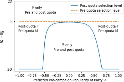
Candidates’ valence and party selection rule. X-axis: pre-campaign popularity of party R (SR varies from −1 to 1). Y-axis: difference between the valence of the female and male candidates, θF − θM (varies from |$-2\bar{\theta }$| to |$2\bar{\theta }$|). The dashed line presents the selection rule for c = 0, that is, party R selects the female candidate if |$\theta _{R,k}^{F}-\theta _{R,k}^{M} \ge b$|, and the male candidate otherwise. The solid line presents the selection rule for c > 0, that is, party R selects the female candidate if |$\theta _{R,k}^{F}-\theta _{R,k}^{M} \ge b-SG_{R,k}$|, and the male candidate otherwise.
Up to now, we gave the intuition considering the party that plays second (in stage 3). We now show that this result extends for the average share of female candidates in equilibrium across both parties. For this, we simulate the equilibrium gender pairs characterized in the Online Appendix drawing in each district the valence of candidates. We compute from these simulations the aggregate fraction of female candidates running for election, for different levels of pre-campaign popularity and initial voter gender bias b > 0. Figure 4 plots the aggregate fraction of female candidates for both the cases of without (panel A) and with (panel B) a cost for deviating from the parity rule. As shown in panel A, the aggregate fraction of female candidates selected by each party is decreasing in voter gender bias b, but independent of the degree of contestability in the absence of gender quotas [equal to |$P(\theta _{R,k}^{F}-\theta _{R,k}^{M} \ge b)=1/2-b/(2\bar{\theta })$|]. As shown in panel B, political parties react strategically to the introduction of the parity rule by selecting disproportionately more female candidates in non-contestable districts.
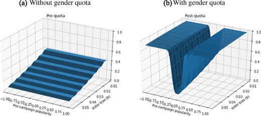
Share of women candidates, competition, and voter gender bias. X-axis: pre-campaign popularity of party R (SR varies from −1 to 1). Y-axis: voter gender bias (b varies from 0.02 to 0.08). Z-axis: share of female candidates.
Identifying the Sign of Voter Bias
Intuitively, observing the allocation of male and female candidates across contestable and non-contestable districts is informative on the sign of the voter bias. We formalize this intuition in the following proposition (see proof in Online Appendix B):
When there are gender quotas on candidates (c > 0):
the share of female candidates is lower in contestable than in non-contestable districts when b > 0 (voter bias in favor of male politicians);
the share of female candidates is higher in contestable than in non-contestable districts when b < 0 (voter bias in favor of female politicians);
the share of female candidates is the same in contestable and non-contestable districts when b = 0 (no voter gender bias).
In Online Appendix C, we introduce intrinsic party bias in our model: parties have a direct utility cost when women sit in the Parliament. We show that this affects the distribution of female candidates across safe and the least winnable districts in the absence of gender quotas. After the introduction of gender quota, we find a pattern similar to Proposition 1 where the share of female candidates in contestable districts is lower than in non-contestable districts (both safe and least winnable districts) when voters are biased against women.
In the next section, we take Proposition 1 to the data and test for the sign of the voter bias in French Parliamentary elections.
5. Empirical Evidence on Strategic Party Behavior and Voter Bias
For testing Proposition 1, we exploit two important institutional features of elections in France. First, gender quotas on candidates were introduced in French Parliamentary elections in 2000. Second, the timing of elections—where Parliamentary elections are in the wake of Presidential elections since 2002—provides us with precise measures of contestability across electoral districts, which we present in Section 5.1. In Section 5.2, we find strong empirical evidence that parties are more likely to select male candidates in contestable districts after the introduction of gender quotas, which indicates that parties strategically react to a voter bias in favor of male candidates. In Section 5.3, we rule out alternative explanations: in particular, the share of female candidates is the same across contestable and non-contestable districts before the introduction of the gender quota. As additional evidence consistent with the voter-bias model, we find in Section 5.4 that elected women have a higher activity level in Parliamentary work than men.
5.1. Measuring Contestability
As already mentioned in Section 2, our main measure of contestability relies on candidates’ parties’ vote shares in the Presidential election preceding the Parliamentary election. Using the previous Presidential election rather than the previous Parliamentary election takes into account swings or alternance occurring in French politics (Murray, Krook, and Opello 2012). The main Left and Right parties reached the runoff of the Presidential elections in all years, except in 2002 and 2017. When both parties reached the runoff of the Presidential election, we define as contestable districts for which the vote margin between the Left and the Right parties in the runoff of the previous Presidential election was between −3 and +3 percentage points. For 2002 and 2017, we instead use Left and Right candidates’ scores in the first round of the Presidential election (and again define as contestable a district in which vote shares were between −3 and +3 percentage points). Using this ±3 cutoff in vote shares, we obtain an average fraction of contestable districts of 28% over the post-quota Parliamentary elections.
We first check that our measure of contestability indeed predicts well the actual tightness of the Parliamentary election in the same district. For this, we simply regress either a dummy for ex-post tight elections or the difference in vote shares between the Left and Right candidates in each district and Parliamentary election, on our dummy indicating ex-ante contestable districts. Online Appendix Table A.7 presents the detailed results. The contestable dummy predicts well the tightness of the election. We find that when the vote margin between the Left and the Right parties in the runoff of the previous Presidential election was between −3 and +3 percentage points, the probability of a tight Parliamentary election in the same district increases by around 33–34 percentage points (28 percentage points when including district fixed effects), as compared to a 28% sample average of tight Parliamentary elections. Similarly, the vote share margin between the Left and the Right parties in the runoff of the Parliamentary election decreases by 8 percentage points (6 percentage points when including district fixed effects), a large effect given the sample vote margin of 12%.
When we compare candidates’ selection before and after the gender quota introduction in Section 5.3, we use ex-post measures of contestability rather than ex-ante measures. Before 2000, the time lag between the Parliamentary election and the previous Presidential election is longer than after 2000. As we do not have data on district-level polls to fill this time gap, we cannot build equally precise measures of ex-ante contestability before and after the gender quota introduction. To avoid that the before–after comparison in Section 5.3 is confounded by a change in precision of our ex-ante contestability proxy, we then use ex-post contestability that is identically measured before and after 2000. In Online Appendix B, we show that the model-based test is also valid when using ex-post vote shares.
5.2. Female Candidates in Contestable versus Non-Contestable Districts
The upper panel of Table 4 reports the estimation results under different specifications. In column (1), we control for election × party fixed effects only. In column (2), we introduce the score of the party in the previous Presidential election. We include controls for candidates’ age, education, and past occupation in columns (3)–(6), for political experience in columns (4)–(6), for gender earnings gaps at the district × election level in columns (5) and (6), and for district fixed effects in column (6).
Electoral contestability and selection of male/female candidates.
| (1) | (2) | (3) | (4) | (5) | (6) | |
|---|---|---|---|---|---|---|
| Panel A: candidates’ selection | Female candidate? | |||||
| Contestable | −0.053*** | −0.066*** | −0.050*** | −0.042** | −0.040** | −0.033** |
| (0.017) | (0.017) | (0.017) | (0.017) | (0.017) | (0.013) | |
| Election × party fixed effects | Yes | Yes | Yes | Yes | Yes | Yes |
| Presidential party vote share | No | Yes | Yes | Yes | Yes | Yes |
| Age, education, occupation | No | No | Yes | Yes | Yes | Yes |
| Incumbent, first run, government exp., local mandate | No | No | No | Yes | Yes | Yes |
| Gender earnings gap | No | No | No | No | Yes | Yes |
| District fixed effects | No | No | No | No | No | Yes |
| Observations | 3,880 | 3,880 | 3,880 | 3,880 | 3,880 | 3,880 |
| R2 | 0.047 | 0.073 | 0.130 | 0.175 | 0.178 | 0.377 |
| Panel B: local pool of candidates | Gender gap high-skill occupation—local politicians | |||||
| Contestable | −0.006 | −0.005 | −0.003 | −0.002 | −0.001 | 0.001 |
| (0.004) | (0.004) | (0.004) | (0.004) | (0.004) | (0.002) | |
| Election × party fixed effects | Yes | Yes | Yes | Yes | Yes | Yes |
| Presid. party vote share | No | Yes | Yes | Yes | Yes | Yes |
| Age, education, occupation | No | No | Yes | Yes | Yes | Yes |
| Incumbent, first run, government exp., local mandate | No | No | No | Yes | Yes | Yes |
| Gender earnings gap | No | No | No | No | Yes | Yes |
| District fixed effects | No | No | No | No | No | Yes |
| Observations | 3,880 | 3,880 | 3,880 | 3,880 | 3,880 | 3,880 |
| R2 | 0.051 | 0.056 | 0.071 | 0.075 | 0.093 | 0.502 |
Notes: This table presents estimates from regressions of candidates’ gender (panel A) and of the gender skill gaps among local politicians (panel B) on a proxy for contestable districts, and control variables. When both the Right and Left parties reached the runoff of the previous Presidential election, we define as contestable districts for which the vote margin between both parties in the runoff of the Presidential election was between −3 and +3 percentage points. For 2002 and 2017, we instead use Left and Right candidates’ scores in the first round of the presidential election (and again define as contestable a district in which vote shares were between −3 and +3 percentage points). In panel A, the dependent variable indicates whether the candidate is a woman. In panel B, the dependent variable is the gender gap in the share of municipal council members with high-skill occupation (over all municipalities in the district). Regressions include election × party fixed effects. Columns (2)–(6) include the vote share obtained by the candidate’s party in the previous Presidential election. Columns (3)–(6) include candidates’ age, and dummies for elite university education and high-skill occupations. Columns (4)–(6) include dummies for incumbents, first-time candidates, former government members, and local mandate as additional controls. Columns (5) and (6) also control for residualized gender earnings gaps in the same district in the year before the election. Column (6) also includes district fixed effects.The sample is restricted to candidates from the main Left and Right party coalitions. Regressions are at the candidate–electoral district level over the Parliamentary elections between 2002 and 2017. Standard errors presented in parentheses are clustered at both the candidate and district–election levels. *, **, and *** denote significance at the 10%, 5%, and 1% levels, respectively.
We find that our parameter of interest—the coefficient β —is negative, stable across specifications, and statistically significant at least at the 5% confidence level. After the introduction of gender quota in 2000, the share of female candidates is between 3 and 6 percentage points lower in contestable districts (than in non-contestable districts). This amounts to a significant 9%–18% reduction from the average post-quota share of female candidates (35%). In column (5), we further control for the district-level gender earnings gap before the Parliamentary election. The coefficient is stable, which further confirms that our result is not driven by confounding factors, where contestable districts are also districts with higher voter bias against women. In column (6), we further control for permanent unobserved characteristics of districts with the introduction of district fixed effects. Again we find robust results when we leverage within-district changes in contestability only. We view these results as strong support for b > 0—that is, that voters are biased in favor of male candidates.
We view our results as complementary to those in Folke and Rickne (2016) and Esteve-Volart and Bagues (2012), who find that stronger electoral competition improves women’s position on the ballots of closed-list elections. These differences might suggest that the implications of electoral competition for women’s representation in the Parliament depend on the electoral system: unlike single-member majoritarian elections, individuals vote over a bundle of candidates in closed-list elections, and it is unclear theoretically how gender-biased voters should react to the presence of, say, a low fraction of female candidates on a given list. We leave this interesting question for future research.46
5.3. Alternative Explanations and Robustness
The main alternative explanation of our empirical test is that parties are constrained in their political selection by the local pool of potential candidates, and that these constraints are stricter when looking for female candidates in contestable districts. The evidence in Table 4 already controls for permanent unobserved differences across districts and thus for stable differences in the local pool of candidates. We now provide three extra pieces of evidence that allow us to further rule out this alternative explanation.
First, we note that the vast majority of candidates for Parliamentary elections hold a local mandate. This allows to characterize the local pool of potential candidates (available after 2000 only). We use the skill-content of the occupations of all mayors and members of the municipality councils in the same districts. For every Parliamentary election and for each party, we compute the share of male local politicians with an high-skill occupation, and the same high-skill share among female local politicians. We then take the corresponding gender gap in high-skill occupation at the district × election × party level, and use this gap as our left-hand-side variable in a regression similar to equation (7). The lower panel of Table 4 reports the results. We find that contestability is essentially unrelated to the gender gap in high-skill occupation among local politicians, whatever the specification.
Second, we use the pre-quota period as a placebo test. Our theoretical model predicts that in the absence of gender quotas, parties should not take into account the local electoral competition when selecting their candidates. We thus run the same regression as equation (7) on the pre-quota election in 1997. As discussed in Section 5.1, we use ex-post measures of contestability to ensure a similar precision of our variable of interest before and after the gender quota introduction.47 Consistent with the prediction of our model, the upper panel of Table 5 shows that the district contestability is not significantly related to the pre-quota probability that the candidate is a woman. This contrasts sharply with the ex-post contestability effect in the 2002 Parliamentary election, reported for the sake of comparability in the lower panel. While Table 5 is restricted to the elections just before and just after the gender quota introduction, we find robust results for the contestability effects across all Parliamentary elections in Figure 5. In every election before 2000, the contestability effect is small and not statistically significant. In every post-quota election, the contestability effect is larger, although less precisely estimated in 2017.
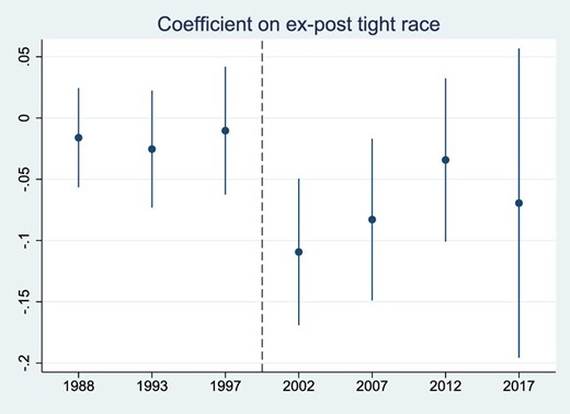
Electoral contestability and selection of male/female candidates, election by election. This figure presents estimates from regressions of candidates’ gender on an ex-post proxy for contestable districts, and control variables. Races are ex-post tight when the vote margin between parties in the runoff of the Parliamentary election was between −3 and +3 percentage points. We run separate regressions for each election year. Regressions include controls as in column (5) of Table 5: election × party fixed effects, the vote share obtained by the candidate in the runoff, candidates’ age, dummies for elite university education and high-skill occupations, dummies for incumbents, first-time candidates, former government members, and local mandate, and residualized gender earnings gaps in the same district in the year before the election. The sample is restricted to candidates from the main Left and Right party coalitions. Regressions are at the candidate-electoral district level over the Parliamentary elections between 1988 and 2017. Standard errors are clustered at both the candidate and district-election levels. Vertical lines around the estimates are at the 95% confidence interval. The dashed vertical line in black indicates the introduction of the gender quota in the year 2000.
Ex-post tight races and selection of male/female candidates—1997 versus 2002.
| (1) | (2) | (3) | (4) | (5) | |
|---|---|---|---|---|---|
| Panel A: 1997 election (pre-quota) | Female candidate? | ||||
| Ex-post tight race | −0.004 | −0.001 | −0.001 | −0.009 | −0.010 |
| (0.026) | (0.026) | (0.028) | (0.027) | (0.027) | |
| Election × party fixed effects | Yes | Yes | Yes | Yes | Yes |
| Candidate vote share | No | Yes | Yes | Yes | Yes |
| Age, education, occupation | No | No | Yes | Yes | Yes |
| Incumbent, first run, government exp., local mandate | No | No | No | Yes | Yes |
| Gender earnings gap | No | No | No | No | Yes |
| Observations | 928 | 928 | 928 | 928 | 928 |
| R2 | 0.044 | 0.059 | 0.102 | 0.160 | 0.160 |
| Panel B: 2002 election (post-quota) | Female candidate? | ||||
| Ex-post tight race | −0.104*** | −0.116*** | −0.102*** | −0.110*** | −0.109*** |
| (0.030) | (0.030) | (0.031) | (0.031) | (0.030) | |
| Election × party fixed effects | Yes | Yes | Yes | Yes | Yes |
| Candidate vote share | No | Yes | Yes | Yes | Yes |
| Age, education, occupation | No | No | Yes | Yes | Yes |
| Incumbent, first run, government exp., local mandate | No | No | No | Yes | Yes |
| Gender earnings gap | No | No | No | No | Yes |
| Observations | 824 | 824 | 824 | 824 | 824 |
| R2 | 0.027 | 0.129 | 0.189 | 0.242 | 0.243 |
Notes: This table presents estimates from regressions of candidates’ gender on an ex-post proxy for contestable districts, and control variables. Races are ex-post tight when the vote margin between parties in the runoff of the Parliamentary election was between −3 and +3 percentage points. In panel A (respectively, B), we analyze the 1997 election (respectively, 2002 election). Regressions include election × party fixed effects. Columns (2)–(5) include the vote share obtained by the candidate in the runoff. Columns (3)–(5) include candidates’ age, and dummies for elite university education and high-skill occupations. Columns (4) and (5) include dummies for incumbents, first-time candidates, former government members, and local mandate as additional controls. Column (5) also controls for residualized gender earnings gaps in the same district in the year before the election. The sample is restricted to candidates from the main Left and Right party coalitions. Standard errors presented in parentheses are clustered at both the candidate and district–election levels. *, **, and *** denote significance at the 10%, 5%, and 1% levels, respectively.
Third, we use candidates not affiliated with parties as another placebo test, in order to address the concern that the results could be explained by female candidates’ decision to self-select out of competitive environment. Reassuringly, we find that the share of female candidates among party-free candidates and their counts are not significantly related to differences in electoral contestability across districts (Online Appendix Table A.8).
These placebo results further confirm that differences in local supply of candidates are unlikely to explain our results. In particular, several studies emphasize that women may systematically under-perform relative to men in competitive environments (Gneezy, Niederle, and Rustichini 2003; Niederle and Vesterlund 2007), and therefore could refrain from running in contestable districts. We do not find that such effects are large enough to explain the magnitude of the estimates in Table 4. More broadly, the placebo tests for the pre-quota period reported in Table 5 and in Figure 5 allow us to rule out alternative explanations where other time-varying district characteristics would confound the effect of electoral contestability.
Another alternative interpretation is that parties indeed react to the gender quota, but based on biased beliefs about voter preferences. The empirical evidence in Section 3 does not support this alternative interpretation. Indeed, we compare municipalities from the same electoral districts in a given election year, where the same man and woman are candidates, and find that unfavorable voters’ attitudes toward women proxied by municipal-level gender earnings gap correlate well with actual gender gaps in vote shares.
Finally, we show in the Online Appendix that our results are robust to using alternative measures of ex-ante contestability. In our main analysis, we use either the first round or the runoff of the previous Presidential election depending on the election. In Online Appendix Table A.9, we use the same round for all elections, either the first or the runoff, and obtain robust results. In Online Appendix Table A.10, we consider alternative score cutoffs for separating contestable and non-contestable districts and again find robust results. We also show in Online Appendix Table A.11 that results are robust when excluding the 2017 election, when the nature of electoral competition switches from a two-player to a multi-player game.
5.4. Gender Gaps in Parliamentary Activity

Parliamentary activity of female versus male elected politicians. This figure plots the coefficient on a female dummy in regressions of parliamentary activity. Intervals centered around the dot correspond to 95% confidence intervals. Each row is a different indicator of parliamentary activity, while the top dot corresponds to the gender gap in the average index of the twelve individual components. Each activity indicator ranges from 1 to 10, and the gender gap should be interpreted as changes in average rank position of women compared to men in the distribution of activity. We add as regression controls election × party fixed effects, year–month fixed effects, and geographical department fixed effects. Standard errors are clustered at the individual politician level. Total sample size amounts to 52,828 observations. Online Appendix Table A.12 reports detailed estimation results.
To the extent that the indicators of Parliamentary activity are relevant proxies for politicians’ valence (in particular for their effort at work), the results in Figure 6 are consistent with the notion that female elected politicians have higher valence than male elected politicians. This provides further support for the voter bias mechanism of our model.49
To sum up, our model-based tests provide strong evidence for the existence of a voter bias in favor of male politicians in French Parliamentary elections. The results highlight that parties strategically internalize voters’ preferences, and provide an explanation for why they find it optimal to pay fines instead of selecting an equal number of female and male candidates. This ultimately reduces the presence of women among elected politicians.
The results also highlight the interaction between bias and electoral competition in shaping the selection of women into politics. In the next section, we calibrate the model and quantify in simulations the importance of competition for the effect of gender quotas on women’s representation among elected politicians.
6. Competition and Gender Quotas
We first calibrate our model with reasonable parameter values and match the gender distribution of candidates both before and after the introduction of gender quotas in French Parliamentary elections. We then conduct counterfactual simulations, and confirm that electoral competition significantly restricts the quota-induced increase in the share of women among elected politicians.
6.1. Calibration
To calibrate our model of electoral competition, we need to choose two core parameters—the voter bias (b) and the cost of deviation from gender parity (c)—, as well as the shape and dispersion of the distributions of initial ideology (Ik), of valences (θ), and of electoral campaign shock (δk). Table 6 summarizes our choice of calibration parameters.
Calibration parameters.
| Parameter | Symbol | Value | Source of calibration |
|---|---|---|---|
| Voter bias | b | 0.06 | Gender gap in electoral scores |
| Dispersion initial popularity | s.d. Ik | 0.16 | Left–Right vote share margins |
| in Presidential elections | |||
| Dispersion campaign shocks | s.d. δk | 0.06 | Parliamentary residualized scores |
| Support candidates’ types | Θ | 0.05 | Match post-quota |$\%$| of women |
| among candidates and elected MPs | |||
| Cost from gender quotas | c | 0.004 | Match post-quota |$\%$| of women |
| among candidates and elected MPs |
Notes: This table presents values of the parameters for our model. We also report whether the parameters are obtained from our own estimates or calibrated to match specific moments of the data.
We use data on electoral scores to pin down the average voter bias b at 0.06.50 The empirical counterpart of the distribution of initial ideology is the Left–Right vote share margins, which follows a normal distribution with standard deviation 0.16. We also choose a normal distribution for the electoral campaign shock. Its empirical counterpart is the distribution of Parliamentary scores residualized by the the Left–Right vote share margins in the Presidential election. Its dispersion amounts to 0.06. There remains two free parameters: the support of the uniform distribution of candidates valence (Θ) and the cost of gender quotas. We conduct a grid search to choose them and match the share of women among candidates in the post-quota period. Setting Θ = 0.05 and c = 0.004 yields 34% of women among candidates, and 28% of elected women in the model. Given the parsimony of the model, the match with the data is reasonable.
6.2. Simulations
Table 7 shows the share of women among candidates (in column 1) and among elected MPs (in column 2), both in the data and in our simulations. Panel A reports the shares in the data in the pre-quota and post-quota periods. Panel B reports the simulation results from the baseline calibration. When we set c = 0, the model predicts that the share of women is 8%, both among candidates and among elected politicians. This is reasonably close to the pre-quota data.
Model simulations.
| (1) | (2) | |
|---|---|---|
| |$\%$| Female candidates | |$\%$| Females elected | |
| Panel A: data | ||
| Pre-quota | 10 | 7.5 |
| Post-quota | 35 | 20 |
| Δ quota | +25 | +12.5 |
| Panel B: baseline simulation | ||
| Pre-quota | 8 | 8 |
| Post-quota | 34 | 28 |
| Δ quota | +26 | +20 |
| Panel C: counterfactual: more contestable | ||
| Pre-quota | 8 | 8 |
| Post-quota | 29 | 23 |
| Δ quota | +21 | +15 |
| Panel D: counterfactual: less contestable | ||
| Pre-quota | 8 | 8 |
| Post-quota | 39 | 32 |
| Δ quota | +31 | +24 |
Notes: This table presents the share of women among both candidates and elected politicians in the data (panel A), in our calibrated model (panel B), and in counterfactual simulations of our model with more (panel C) and less (panel D) electoral competition among the two main parties.
In panels C and D of Table 7, we report the results of counterfactual simulations where we vary the intensity of electoral competition. In panel C, we reduce the dispersion of initial ideology from 0.16 to 0.14, and hold constant the other parameters. Electoral competition intensifies, and the share of contestable electoral districts increases by 10% (3 percentage points). This leaves unchanged the share of women in the pre-quota environment. However, in the presence of gender quota, higher competition decreases the share of women among candidates (and elected politicians) by 5 percentage points (compared to the baseline). As there are now more contestable districts, parties select significantly fewer women. Overall, while the gender quota increases the share of elected women by 20 percentage points in the baseline simulation, the difference post − pre quota is 15 percentage points in the counterfactual simulation. In other words, the quota-induced increase in women among elected politicians is 25% lower when the share of contestable districts increases by 10%.
In panel D, we conduct the symmetric counterfactual simulation where the standard deviation of the initial ideology increases to 0.18. Electoral competition is less intense, and there are less contestable districts. The quota-induced increase in female MPs is significantly larger than in the baseline simulation.
Finally, in Online Appendix Section C.3, we present the same simulations for the extension of our model with intrinsic party bias (such that political parties enjoy an additional utility when a male politician is elected as compared to a female politician). As expected, the share of female candidates and politicians is lower in the presence of party bias. However, we still observe in simulations that electoral competition hinders the effectiveness of the parity rule in boosting the presence of women in politics.
7. Conclusion
We study and quantify the implications of voter bias and electoral competition for the gender composition of politicians. We first provide empirical evidence that survey-based measures of unfavorable voters’ attitudes toward women and local gender earnings gaps correlate negatively with the share of female candidates in French Parliamentary elections. In addition, we find that within an electoral district and election, female candidates obtain lower votes compared to their male competitors in high gender earnings gap municipalities. We then propose a model of political selection with voter bias, and show theoretically that electoral competition pushes political parties to tilt the allocation of the most contestable districts toward either male or female candidates depending on voters’ gender preferences in the presence of gender quotas on candidates.
Exploiting the 2000 introduction of gender quotas in France, we find strong empirical support for a strategic party response to a voter bias in favor of male candidates. In the most contestable districts, the electoral cost of selecting women when there is a voter bias in favor of male candidates outweighs the cost of the fine post-quota, and we find that this effect is large enough for explaining why the main two parties select on average post-quota only 35% of female candidates, significantly below the objective of the Parity Law. We do not see the forces highlighted in our paper as specific to gender per se. They might also generalize to the analysis of minority representation in politics. Finally, we highlight that competition might hurt women’s representation in politics—and the effectiveness of gender quotas—when voters have a preference for male politicians.
Overall, our finding that voters’ attitudes toward gender affect gender gaps in politics—both for differences in electoral scores and for differences in the gender composition of candidates—has important consequences, and suggests that slow-moving voters’ attitudes might be an important factor that limits convergence toward a gender parity among politicians over the world.
Notes
The editor in charge of this paper was Paola Giuliano.
Acknowledgments
This paper was previously circulated under the title “Voter Bias and Women in Politics”. We thank Jerome Adda, Alessandra Casarico, Vincenzo Galasso, Nicola Gennaioli, Eliana La Ferrara, Massimo Morelli, Tommaso Nannicini, Salvatore Nunnari, Daniele Paserman, Paola Profeta, Vincent Pons, Roland Rathelot, Alexandra Roulet, Guido Tabellini, Clemence Tricaud, Paola Giuliano, three anonymous referees, and seminar participants at Alp-Pop 2020, Bocconi, Boston University, Chicago Booth, Crest, EIEF, Heriot–Watt University, Mannheim University, and Venice Summer Institute 2019 for very helpful comments. We thank Mathieu Fouquet and Innessa Colaiacovo for providing excellent research assistance. All remaining errors are our own. Thomas Le Barbanchon is also affiliated with IGIER, CEPR, J-PAL, and IZA and Julien Sauvagnat is also affiliated with IGIER and CEPR.
Footnotes
Existing evidence on the under-representation of women in powerful and well-paid positions is not restricted to politicians, and covers a wide range of other occupations, including top management in big corporations (e.g., Bertrand and Hallock 2001) and academia (Bagues, Sylos-Labini, and Zinovyeva 2017).
Prior work documents gender differences in policy preferences (e.g., Lott and Kenny 1999; Miller 2008; Alesina and Giuliano 2011; Funk and Gathmann 2015). However, differences in policy preferences do not necessarily need to translate into differences in policy-making (Ranehill and Weber 2017). While several studies report significant gender differences in policy-making in developing countries (e.g., Chattopadhyay and Duflo 2004; Clots-Figueras 2011, 2012; Brollo and Troiano 2016), the evidence is more mixed in the context of Western democracies (Ferreira and Gyourko 2014; Bagues and Campa 2021; Baskaran and Hessami 2019; Lippmann 2019).
Krook (2018, p. 187) summarizes the state of the literature in her handbook chapter as: “In the case of gender, existing work is ambivalent as to the nature and effects of [voter] bias against female candidates.”
We do not take a stand on the source of this bias. It might, for instance, reflect traditional views on the role of women in society, taste-based discrimination, or statistical discrimination. See, for example, Broockman and Soltas (2018) and Eymeoud and Vertier (2018) for recent studies aiming at identifying taste-based statistical discrimination in electoral data. It might also be that some voters prefer to vote for a male politician due to differences in policy preferences.
While informative, survey experiments are often carried out using small samples, and raise bias concerns, such as, for instance, demand effects (Kane and Macaulay 1993).
Another approach has been to infer the presence of voter gender bias by looking at gender gaps in electoral outcomes. Recent evidence includes Esteve-Volart and Bagues (2012), Hogan (2010), Fréchette et al. (2008), and Murray, Krook, and Opello (2012). However, gender electoral gaps are equilibrium objects, which makes it difficult to credibly identify voter bias from other factors, such as, for instance, the role of parties (which may, for instance, select women in less winnable positions/districts), or gender differences in other candidates’ attributes. Recent studies (Kunovich 2012; Stegmaier, Tosun, and Vlachova 2014) leverage open-list proportional systems with ordered lists in Central and Eastern Europe to compare voters’ and parties’ preferences over candidates’ gender.
Note that the within-candidate design does not rely on time variation across election years. Instead, it relies on variations across municipalities within an electoral district in a given election year.
This prediction also applies to situations in which parties face strict quotas on the share of female and male candidates.
Single-member constituencies are pervasive across the world, and also include, for instance, the United States, the United Kingdom, Canada, Japan, India, Australia, and Pakistan.
A growing literature in economics and finance studies the implications of gender quotas in other contexts, such as, for example, board of directors (Ahern and Dittmar 2012; Bertrand et al. 2018), academia (Antecol, Bedard, and Stearns 2018), and evaluation committees (Bagues and Esteve-Volart 2010).
In practice, members of the Parliament might hold their office for less than 5 years in the case of dissolution of the Assemblée Nationale: in our sample period, the 1997 election was called in advance by president Jacques Chirac. An exception to the two-round majoritarian system was the 1986 Parliamentary election for which the voting system combines a majoritarian and proportional rule and took place in one round only.
Data on candidates and electoral outcomes are not available before 1988 in digitalized format.
Over the elections in our sample, the Left coalition is mainly composed of candidates from the Parti Socialiste (PS, 84%) and Parti Radical de Gauche (PRG, 12%). The Right coalition is mainly composed of candidates from the Rassemblement pour la République (RPR, 79%) and the Union pour la Démocratie Francaise (UDF, 20%) until 1997, Union pour la Majorité Présidentielle (UMP) in 2002, 2007, and 2012, and Les Républicains (LR) in 2017.
We exclude from our main sample La République en Marche (LaREM) and the Movement Démocrate (MoDem) from the 2017 election even though this centrist coalition has obtained the majority of seats in the Parliament in 2017. For the sake of simplicity, we abstract in the model presented below from the complications of strategic voting with more than two parties (which would be appropriate in the case of the 2017 election). Note, however, that we find virtually the same empirical results when including the candidates of LaREM and MoDem in the sample, or, alternatively, excluding the 2017 Parliamentary election from the sample.
As an illustration, even though the Front National (FN) has obtained vote shares between 10% and 20% in first rounds of Presidential elections over the sample period, the majoritarian voting rule makes it almost impossible for their candidates to win seats in the Assemblée Nationale. Note that the Front National—unlike the two main Left and Right coalitions—presented around 50% of female candidates in the 2002 (and following) elections, as required by the Parity Law voted in France in 2000 (described below), very much in line with the idea explored in this paper that electoral competition is an important factor restricting the probability of running for elections for female politicians.
For example, if there are only 35% of female candidates running for election in a given party, the difference between the number of female and male candidates is 30 percentage points, in which case the fine amounts to a 15 percentage point cut on the amount of public funding received by the party. While public funding is the main source of financing for the main French political parties, they also raise private funds through membership fees, and donations from elected representatives and individuals (a ceiling on individual donations was set at 7,500 euros a year). See François and Phélippeau (2018) for more details about party funding in France.
Gender is missing in 1993 and 1997. We then retrieve gender either from other elections in the case of candidates running several times for elections (and from the Assemblée Nationale website for elected politicians), or from candidates’ first names. There is almost no uncertainty in the mapping between first names and gender in the case of French candidates.
We retrieve date of birth and occupation for elected candidates from the Assemblée Nationale website. We complement missing information with data from the Centre de Données Socio Politiques (CDSP) maintained at Sciences Po. Data on the occupations of candidates for the 1997 Parliamentary elections were digitalized within the ANR project La coordination stratégique et le scrutin à deux tours : Electeurs, partis et règles électorales en France, supervised by Annie Laurent. We thank Fréchette et al. (2008) for providing us with data on candidates’ age for the Parliamentary elections in 2002 and 2007 and Clémence Tricaud for sharing with us the Répertoire National des Elus from which we can recover date of birth and occupation for politicians who also get elected in municipal elections in 2001, 2008, or 2014. We scrapped Wikipedia pages for the remaining cases. When we cannot retrieve date of birth or occupation for a given candidate, we include a dummy for missing date of birth or missing occupation in the regressions presented below. Date of birth (respectively, occupation) is missing for 10% (respectively, 15%) of candidates in our sample. All regression results are virtually unchanged when we restrict our attention to candidates with non-missing information on age and occupation.
This corresponds to the third group of the French occupation classification Cadres et professions intellectuelles supérieures.
We retrieve the data from alumni directories of these schools. These institutions fill in a large fraction of the most prestigious jobs in the public administration, in politics, and in the top management of large private and state-owned companies (see e.g., Kramarz and Thesmar 2013).
There are 96 départements in Mainland France, and around 6 electoral districts per département.
The last three waves of the World Value Survey (WVS) comprise the exact same two questions. Reassuringly, the share of French respondents who agree or strongly agree with the statement “On the whole, men are better political leaders than women” is similar in the GGS and in the WVS, respectively, 17% and 21%. One may also wonder whether France is an outlier in terms of the share of respondents who agree (or strongly agree) with the statement. France ranks at the 20th percentile in the distribution of countries with available data in the WVS. For instance, this share is equal to 11% in Sweden, 17% in Germany, 18% in the United States, 20% in the United Kingdom and in Italy, 28% in Brazil, 42% in Japan, 54% in China, and 60% in Russia.
We first regress yearly earnings on workers’ age, four-digit occupation, and employers’ industry. We then take the local average of residuals of either male or female workers and compute the difference. In line with prior work, we find that age, occupation, and industry absorb around two-thirds of the raw earnings gaps; see Blau and Kahn (2017). French employment registers (DADS) are available starting from 1996. We thus use local earnings gaps measured in 1996 for the Parliamentary elections in 1988 and 1993.
One potential concern from using “Do you agree with the statement: men are better political leaders than women” is that this statement might also reflect reverse causality, if, for instance, voters’ exposure to female politicians improves their perceptions about female leader effectiveness (Beaman et al. 2009; Baskaran and Hessami 2018). While we cannot formally rule out this possibility, finding robust results when using either survey data on attitudes toward women on labor markets or local gender earnings gaps mitigates the reverse causality issue.
Including this control addresses, for instance, the concern that districts in which individuals share the view that “Men are better political leaders than women” might be arguably easier to win for Right candidates, and the Right party tend to allocate male candidates to the most winnable districts. However, if anything, the size of the coefficient increases once we control for candidates’ affiliated party scores in the Presidential election.
One potential concern might be that gender earnings gaps reflect women’s wages in the private sector, and therefore affect the local supply of politicians, not through beliefs, but through equilibrium effects on labor markets. For instance, a Roy model of sector selection could predict that more women would select into politics when local private-sector wages are lower (and gender earnings gap therefore larger). However, if this is the case, this would lead us to underestimate the negative effect of (unfavorable) voters’ attitudes toward women on women’s participation into politics when using gender earnings gaps, given that we would have obtained an even more negative coefficient in the absence of sector-selection effects.
Female candidates in districts with less favorable attitudes toward women might not want to run in these districts because they think it is not appropriate for women to do so.
Suppose, for instance, that the expertise of female politicians is lower in districts in which voters tend to favor male politicians. In this scenario, we would then wrongly attribute differences in vote shares to voters’ attitudes, while they would simply reflect unobserved differences in the expertise of male versus female politicians. Suppose instead—as it is the case in the model of political selection presented below—that parties refrain from selecting female candidates in districts in which voters tend to favor male politicians. In this scenario, the selection introduces a downward bias in the relationship between voters’ attitudes and gender gaps in vote shares.
Still, it could be that even within party, men and women campaign on different policies, and that voters in municipalities with lower gender earnings gaps prefer policies proposed by women. While we can control for party affiliation, we do not observe policies proposed by each candidate.
Furthermore, we do not find any statistically significant relation between gender attitudes (as measured in the GGS or in gender earnings gap) and the Presidential score of the Right party across department.
Using the cross-département correlation between gender earnings gaps and beliefs obtained in Online Appendix Table A.2, we can estimate that a 10 percentage point increase in the belief that “Men are better political leaders than women” is associated with a 1.2 (0.078 * 10/0.613) percentage point decrease in vote shares for female candidates.
We do not take a stand on the precise mechanisms through which voters’ attitudes affect gender gaps in vote shares. While the estimates indicate that unfavorable attitudes toward women, as proxied by local gender earnings gaps, lead voters to vote less for women, these findings might also partly reflect the fact that female candidates spend less time campaigning in municipalities where they know that gender bias is higher. This could be the case if they expect the returns of their efforts (in terms of votes won) to be lower or discussions with voters to be less pleasant there. They may also have fewer resources in these municipalities, for example, they may have a harder time recruiting local volunteers for door-to-door canvassing and other field activities there. We leave the quantification of the relative importance of these effects outside the scope of our paper, and interpret our estimates as the sum of the direct and indirect impacts of voters’ attitudes on gender gaps in vote shares.
There are around 5,200 municipalities (out of 36,500 in total) with above 2,000 inhabitants (the administrative cutoff for a town in France).
For the sake of simplicity, we abstract from the two-round majority voting rule of French Parliamentary elections, and start directly with a model of electoral competition in which two parties compete for winning seats in the Parliament in one-round elections.
One implicit assumption in the objective function (3) is that parties equally care for every seat they obtain. Obtaining the majority of seats in the Parliament allows the winning coalition to form the government, which is arguably an additional source of utility introducing theoretically a discontinuity in the party objective of around 50% of the seats. However, it is reasonable to abstract from this discontinuity in the case of French Parliamentary elections given that in reality there is generally no uncertainty on the fact that the party winning the previous Presidential election will also win the majority of seats in the following Parliamentary election.
Restricting the choice to two local candidates in each district is without loss of generality. Alternatively, one may consider local pools of female and male candidates with heterogeneous valence, in which case the party would then simply choose between the male and female candidates with the highest valence.
Note that this is a lower bound on the true fraction of local candidates to the extent that some local candidates might run for the first time in politics or might hold other types of local political mandate that we do not observe in our data. Moreover, a vast majority of (repeat) candidates run in the same district: 96% of candidates running in several elections run in the same electoral district.
We test implications of this assumption in Section 5.4.
We implicitly assume that the degree of voter bias does not depend on the ideology of voters. This is consistent with the evidence in Table 3, column (5), where we find that our empirical proxy for voter bias has the same effect on the vote shares of female candidates from the Left and Right parties.
We derive below a test for identifying the sign of b in the data. As it will be clear, assuming that b is homogeneous across districts is without loss of generality when solving for the equilibrium of the game. When b is heterogeneous across districts, the test presented in Section 5 then identifies the average voter bias b (under the assumption that there is no correlation between the cross-district distributions of bk and the distribution of ideology Ik).
When |$|b|>2\bar{\theta }$|, the selection of candidates is trivial and boils down to selecting only male candidates when |$b>2\bar{\theta }$|, and only female candidates when |$b<-2{\bar{\theta }}$|, whatever the relative values of θL and θM.
This can be interpreted as the voters’ reaction during the campaign to candidates’ profile and attitude, such as her/his oral ability.
Assuming that parties choose their candidates sequentially is not necessary, but allows to obtain a unique equilibrium for all parameter values. Alternatively, when parties choose simultaneously their candidates, there are multiple equilibria for some parameter values (including equilibria in which parties play mixed strategies). Note that we find virtually the same results for the aggregate share of female candidates in the calibration and in simulations presented below when parties choose their candidates simultaneously, and we assign equal weights to each equilibrium in cases with multiple equilibria.
When b = 0, the equilibrium fraction of female and male candidates is 1/2.
We discuss the optimal strategy of party L in stage 2 and characterize the equilibrium in the Online Appendix.
As an illustration in the context of minorities, Adida, Laitin, and Valfort (2016) provides lab-in-the-field experimental evidence on how anti-Muslim prejudice depends on the local share of Muslims. Similarly, one could imagine that voters (including those who are gender-biased) in a closed-list election might prefer to vote for a list with a positive number of women rather than for a list with men only. Voters might appreciate diversity, among other things, but such a preference can be expressed only when they are faced with a list rather than with an individual candidate. This argument is in the spirit of the changes made in the nomination process for the assignment of Nobel prizes, where encouraging voters to consider multiple discoveries might have increased the share of women nominated (see link here: https://www.nature.com/articles/d41586-019-02988-5).
The Presidential election before the 1997 Parliamentary election took place in 1995, while the 2002 Parliamentary election took place a few weeks after the 2002 Presidential election.
The data are publicly available in digitalized format from the website: www.nosdeputes.fr. We use each indicator of activity recorded by the French Parliament.
These results are counterfactual to an alternative model without voter bias (b = 0) and heterogeneous support for the valence of female versus male candidates, in which political parties would tend to select male candidates in contestable districts under gender quotas because on average the valence of male candidates is higher than the valence of female candidates. This alternative model predicts instead that the valence of female MPs should be lower than the valence of male MPs.
We showed in the previous section that b is positive. Conditional on the campaign electoral shock, b/4 can be interpreted as the difference in vote share between a male and female candidates. We then use regressions of vote shares on female dummy to inform the calibration of b. We obtain a coefficient around 0.015 once controlling for candidates’ characteristics; see the last columns of Online Appendix Table A.13.
