


Abstract
Using detailed firm-level transactions data for UK imports, we find that invoicing in a vehicle currency is pervasive, with more than half of the transactions in our sample invoiced in neither sterling nor the exporter’s currency. We then study the relationship between invoicing currencies and the response of import unit values to exchange rate changes. We find that for transactions invoiced in a vehicle currency, import unit values are much more sensitive to changes in the vehicle currency than in the bilateral exchange rate. Pass-through therefore substantially increases once we account for vehicle currencies. This result helps to explain why UK inflation turned out higher than expected when sterling depreciated during the Great Recession and after the Brexit referendum. Finally, within a conceptual framework, we show why bilateral exchange rates are not suitable for capturing exchange rate pass-through under vehicle currency pricing. Overall, our results help to clarify why the literature often finds a disconnect between exchange rates and prices when vehicle currencies are not accounted for.
A set of Teaching Slides to accompany this article are available online as Supplementary Data.
1. Introduction
A well-established fact in the open-economy macroeconomics literature is that the prices of internationally traded goods only react modestly to changes in exchange rates. In other words, the pass-through of exchange rate changes into import and domestic prices is incomplete.1 In a large class of models with nominal rigidities, the currency in which traded goods are priced has implications for the degree of exchange rate pass-through. In the short run, pass-through is complete if prices are set in the exporter’s currency (“Producer Currency Pricing,” PCP), while it is zero if prices are set in the importer’s currency (“Local Currency Pricing,” LCP).2 In the long run, this difference in pass-through disappears if prices are set exogenously in either currency, while it persists if the currency choice is endogenous (Gopinath, Itskhoki, and Rigobon 2010).
Using highly disaggregated firm-level data for UK imports from non-E.U. countries, this paper examines the relationship between the currency of invoicing and exchange rate pass-through. Our contribution is fourfold. First, we show that “Vehicle Currency Pricing” (VCP) is pervasive for UK imports, with more than half of the transactions in our sample invoiced in neither sterling nor the exporter’s currency. VCP has been rarely studied in the pass-through literature because the lack of bilateral invoicing currency data makes it difficult to distinguish between pricing in a vehicle currency or in the partner’s currency (Gopinath 2015).3 Second, we estimate the sensitivity of import unit values to exchange rate fluctuations with a focus on VCP, in addition to pricing in producer or local currencies.4 Third, we address the implications of our findings for inflation. We show that ignoring the currency of invoicing can lead researchers to mismeasure the effects of exchange rate changes on import price inflation. Fourth, we extend the theoretical framework of Engel (2006) to explain exchange rate pass-through in the presence of VCP.
Focusing on the UK economy is particularly well suited for our purposes. First, the sterling nominal exchange rate is freely floating against other major currencies, and it has experienced significant fluctuations over time. Second, we were granted access to a highly disaggregated data set from Her Majesty’s Revenue and Customs (HMRC) which provides the universe of the Cost, Insurance, and Freight (CIF) import transactions of the UK economy. For each transaction, we observe a unique trader identifier, the country of origin, the date of transaction, the ten-digit comcode product identifier, the value (in sterling), and the mass (in kilograms). Most importantly, we observe the currency of invoicing for each transaction from 2010 to 2017 but for non-E.U. transactions only. As we do not directly observe import prices, as a proxy we compute import unit values at the trader-product-currency-origin level. Finally, and crucially for our purposes, we observe a large share of import transactions invoiced in vehicle currencies. VCP accounts for 54.54% of non-E.U. import transactions, whereas PCP and LCP represent 18.33% and 27.13%, respectively.5
Our main results can be summarized as follows. Across all transaction types, we find that short-run pass-through (i.e., within one quarter) is incomplete and low at 17.9%. We then demonstrate that pass-through varies substantially across invoicing choices. Pass-through is large at 62.0% for imports in producer currencies but insignificant for transactions in local currency (sterling). For imports in vehicle currencies, pass-through is low at 24.2% when we estimate it based on the bilateral exchange rate between the exporting and importing countries. But once we let the unit values of the vehicle currency transactions depend on the exchange rate between sterling and the vehicle currency, pass-through is much larger at 59.2% and thus in the same ballpark as for PCP. Using the bilateral rather than the vehicle currency exchange rate therefore substantially underestimates pass-through for goods priced in vehicle currencies. Intuitively, the bilateral exchange rate is an inadequate measure of the relevant exchange rate variation, and it therefore leads to attenuated pass-through estimates.
For long-run pass-through (i.e., after 2 years), our results remain similar. Across all transaction types, pass-through is low at 41.3%. But by invoicing choice, it is large at 70.0% for producer currency transactions and zero for local currency transactions. For transactions in vehicle currencies, pass-through is low at 36.6% when we use bilateral exchange rates, but much higher at 59.0% when we use vehicle currency exchange rates. For each invoicing choice, there is therefore little difference between short- and long-run pass-through. This means pass-through rates across invoicing choices do not converge in the long run. These patterns are consistent with the predictions of models where prices are sticky and firms endogenously choose their currency of invoicing in order to keep their preset price closer to their desired price in periods when they do not adjust (Burstein and Gopinath 2014; Engel 2006; Gopinath 2015; Gopinath et al. 2010; Mukhin 2018).
The finding that bilateral exchange rates are inappropriate in pass-through regressions has recently been emphasized in the literature. According to the “Dominant Currency Paradigm”, firms choose to invoice in a dominant currency, typically the US dollar. It is therefore not the bilateral exchange rate but the US dollar exchange rate that is driving global trade prices (Gopinath 2015; Gopinath et al. 2020). Our results confirm that bilateral exchange rates are unsuitable for explaining import unit values invoiced in vehicle currencies, but our emphasis is on vehicle currencies, as opposed to dominant currencies, in explaining pass-through. As a result, our approach and our findings differ from the Dominant Currency Paradigm in several dimensions.
First, in contrast to Dominant Currency Pricing (DCP), VCP distinguishes between the US dollar as a producer currency and a vehicle currency. Moreover, it considers other vehicle currencies than the US dollar in explaining pass-through. There is, however, a strong overlap between DCP and VCP because the US dollar, which is the dominant currency, is also the main vehicle currency. In our sample, 88.5% of vehicle currency transactions are invoiced in US dollars. The rest is invoiced in 90 other currencies, in particular the euro. Yet, we demonstrate that the behavior of exchange rate pass-through is in fact consistent with both DCP and VCP. On the one hand, as the US dollar is the dominant currency, we confirm that its pass-through is high and of the same magnitude whether it is used as a producer or a vehicle currency. But on the other hand, we find that pass-through is equally high for vehicle currency transactions in non-US dollars. It is therefore the use of vehicle currencies generally, and not the US dollar specifically, that is driving the high pass-through for vehicle currency transactions. Non-US dollar vehicle currencies are far less pervasive than the US dollar, but our contribution is to show that they also matter for pass-through. This finding could be seen as an extension of the results by Gopinath et al. (2020) to vehicle currencies less prominent than the US dollar.
Second, while Gopinath et al. (2020) find that the pass-through of the euro exchange rate is negligible, we provide evidence that the euro exchange rate contributes to explaining UK import unit values invoiced in vehicle currencies. In regressions with bilateral exchange rates, we show that controlling for the US dollar exchange rate helps to increase pass-through estimates, but so does controlling for the euro exchange rate. But while these exchange rates help to push up pass-through estimates, they fall short of replicating the magnitude of our pass-through elasticities based on actual invoicing currencies.
Our results are important because of their implications for import and thus consumer price inflation. To shed light on this issue, we focus on three quarterly episodes of large sterling fluctuations (during the Great Recession, and after the European Sovereign Debt Crisis and the E.U. referendum). We use our estimates to evaluate the dynamic response of import price inflation to these exchange rate shocks. Once we account for invoicing currencies, we can explain why pass-through into import unit values was higher than expected by forecasters and policymakers during the Great Recession and after the E.U. referendum. The reason is that for transactions in vehicle currencies, import unit values respond more to changes in the vehicle currency than in the bilateral exchange rate. And since the US dollar is used extensively as a vehicle currency, the depreciation against the US dollar during the Great Recession and after the E.U. referendum is given a larger weight than import shares would suggest, resulting in higher implied import price inflation. Instead, in the aftermath of the European Sovereign Debt Crisis, we find lower-than-expected pass-through because the fall in inflation induced by the appreciation of sterling against the euro is more than offset by the depreciation against the US dollar.
Our predictions match the actual behavior of consumer and import price inflation after each exchange rate shock. It is indeed well documented that the depreciation of sterling during the Great Recession and following the E.U. referendum increased domestic inflation by more than expected, while the appreciation of sterling after the European Sovereign Debt Crisis reduced it by less than anticipated. During the Great Recession, the Bank of England noted that the surprising strength in inflation was probably reflecting “stronger, or faster, exchange rate pass-through following the fall in sterling”. On 13 June 2017, about 1 year after the E.U. referendum, the Financial Times reported that the jump in inflation was “above analysts’ consensus forecasts”. By contrast, after the European Sovereign Debt Crisis, the Bank of England observed that “import prices have not fallen by as much as might have been expected [...]. The Monetary Policy Committee judges that the earlier appreciation will be associated with somewhat less of a fall in import prices than previously assumed”.6
Our results have therefore implications for the setting of monetary policy. We argue that policymakers should update their “rules of thumb” for predicting how currency fluctuations affect future prices (Forbes, Hjortsoe, and Nenova 2018).7 In particular, they should take into account that when VCP is pervasive, bilateral exchange rates are inappropriate for determining the inflation effects of exchange rate changes for two reasons. First, the pass-through elasticity is larger for transactions priced in vehicle currencies. Second, the weight assigned to that elasticity and therefore the overall effect on inflation will be stronger for countries with larger shares of vehicle currency imports. Put simply, to predict how currency fluctuations affect inflation, policymakers should construct an effective nominal exchange rate that is based on invoicing currency weights, not trade weights.
Lastly, we develop a simple conceptual framework to better understand pass-through estimates in the presence of VCP from a theoretical point of view. Based on Engel (2006), we outline a three-country model in which monopolistic exporters invoice in a vehicle currency. We show that in this setting, prices in the destination country do not solely depend on the bilateral exchange rate but also on a second exchange rate term involving the vehicle currency. Due to triangular exchange rate arbitrage, it is possible to estimate various alternative specifications but all of them include two exchange rate terms. We demonstrate in our data that when only controlling for the bilateral exchange rate, we would find a low pass-through coefficient under VCP. We argue that such a finding should not erroneously be interpreted as “exchange rate disconnect” because, in fact, pass-through is high with respect to the vehicle currency exchange rate.
This paper builds on and contributes to the literature on exchange rate pass-through which typically finds a low degree of pass-through into import prices (Campa and Goldberg 2005; Gopinath and Rigobon 2008) and consumer prices (Campa and Goldberg 2010).8 Within this literature, papers most closely related to our work are those that investigate the relationship between the invoicing currency and pass-through.9 Gopinath et al. (2010) find that pass-through is low for US imports in US dollars and large when priced in non-US dollars. Cravino (2017) shows that exchange rate changes affect the prices of firm-level exports invoiced in the exporter’s currency, but have no effect on export prices set in the destination’s currency. Auer, Burstein, and Lein (2021) and Bonadio, Fischer, and Sauré (2020) study the appreciation of the Swiss franc against the euro in 2015. Auer et al. (2021) find that the consumer prices of imported goods fell to a larger extent in product categories with larger reductions in import prices and a smaller share of import prices invoiced in Swiss francs. Bonadio et al. (2020) show that pass-through into import unit values was complete for goods priced in euros, but incomplete for goods in Swiss francs.10 These studies, however, do not examine vehicle currencies.
Among the papers that emphasize the role of the US dollar as a dominant currency, Gopinath (2015) shows that countries with larger shares of imports invoiced in a foreign currency, and in particular the US dollar, have higher short- and long-run exchange rate pass-through. Using bilateral industry-level trade data combined with country-level data on invoicing currency choices, Gopinath et al. (2020) show that it is not the bilateral exchange rate but the US dollar exchange rate that drives trade prices. They also show that controlling for the peso to the US dollar exchange rate knocks down the effect of the bilateral exchange rate in explaining the prices of Colombian firm-level exports. Consistent with these papers, we challenge the view that bilateral exchange rates are appropriate to evaluate pass-through. But we argue that this view applies not just to the US dollar but to all vehicle currencies in our sample.
To the best of our knowledge, only two papers examine VCP empirically. For New Zealand, Fabling and Sanderson (2015) find that pass-through is high for firm-level exports invoiced in domestic currency and low when priced in local and vehicle currencies. Corsetti, Crowley, and Han (2018) show that destination-specific markup adjustment to changes in bilateral exchange rates is substantial for UK firm-level exports invoiced in the destination’s currency, but non-existent for transactions priced in sterling or a vehicle currency. We differ from these papers by studying import unit values. This allows us to assess the sensitivity of imported inflation to exchange rate shocks depending on invoicing currencies.11
The remainder of the paper is organized as follows. Section 2 describes our firm-level customs data and provides descriptive statistics. Section 3 presents our main empirical results. Section 4 derives the implications of our findings for import price inflation. Section 5 analyzes exchange rate pass-through under VCP from a conceptual point of view and discusses exchange rate disconnect. Section 6 concludes.
We provide an extensive online appendix with additional results. Online Appendix A compares our baseline bilateral pass-through coefficient with population-weighted averages across invoicing choices. Online Appendix B highlights the omitted variable bias in pass-through estimates for producer currency transactions when vehicle currency exchange rates are not accounted for. Online Appendix C provides evidence against the notion of passive exchange rate pass-through. Online Appendix D reports a wide range of robustness checks. Online Appendix E presents results for export unit values, while Online Appendix F describes our findings for export and import quantities. Online Appendix G explains how we calculate our back-of-the-envelope effects of exchange rate shocks on import price inflation. Online Appendix H provides theoretical derivations.
2. Data and Descriptive Statistics
Our data set uses transaction-level customs data for the UK economy. Quarterly consumer price indices and period-average nominal exchange rates are from the International Financial Statistics of the International Monetary Fund.
2.1. Customs Data
Transaction-level CIF imports are obtained from HMRC, a non-ministerial Department of the UK Government responsible for the collection of taxes, the payment of state support, and the collection of trade in goods statistics. Data access is only granted to approved projects and all empirical output is subject to HMRC’s code of statistical disclosure.
For each import transaction, the data set provides us with a unique trader identifier, the country of origin, the transaction date, the five-digit Standard International Trade Classification (SITC) Revision 3 and the four-digit Harmonized System (HS) Revision 2007 classifications, the ten-digit comcode product code (the first eight digits correspond to the Combined Nomenclature), the value (in sterling), the mass (in kilograms) and, most importantly, the currency of invoicing but for non-E.U. transactions only.12 While the trade data are available since 1996, we concentrate our analysis on the 2010–2017 period because reporting the currency of invoicing has only become compulsory since 2010 for non-E.U. imports. Non-E.U. imports represent 50% of total UK imports between 2010 and 2017. At the trader-product-currency-origin level, we aggregate the data at quarterly frequency. Given that import prices are not observed, we compute import unit values by dividing the quarterly transaction value in sterling by the corresponding mass in kilograms.13 As we rely on unit values, we are unable to observe when firms adjust their prices.14
We clean the data in several ways. First, we drop the few transactions for which the currency of invoicing is missing. Second, we exclude the “Not classified” industry (SITC 9), but we keep homogeneous commodities such as “Crude materials” (SITC 2) and “Mineral fuels” (SITC 3) in the sample. Although their prices are determined by world supply and demand (Gopinath 2015), commodities are an important component of UK imports (as shown in Table 3, the combined share of the two SITC categories in non-E.U. imports is equal to 16.11%).15 Third, we drop the observations for which the value of imports is positive but the corresponding quantity is zero. Finally, to minimize the influence of potential outliers, we exclude the 0.5% of observations with the largest and smallest log changes in unit values (i.e., we drop 1% of the sample). Our results remain similar if we instead winsorize the data.
2.2. Descriptive Statistics
As shown in Table 1, our sample between 2010 and 2017 includes 120,429 firms, 16,219 products (at the ten-digit comcode level), and 138 origin countries with a total of 5,792,400 observations.16 These firms import an average of 6.9 different products from 2 origin countries (at the 5th and 95th percentiles, the products per importer are 1 and 25, and the origin countries per importer are 1 and 6).17 The mean import transaction is valued at 213,630 pound sterling in each quarter, or 760.7 pound sterling per kilogram. The mean change in import unit values is equal to 0.8% per quarter.
Summary statistics.
| Mean | Median | Standard deviation | 5th percentile | 95th percentile | |
|---|---|---|---|---|---|
| Importers | 120,429 | – | – | – | – |
| Products | 16,219 | – | – | – | – |
| Origin countries | 138 | – | – | – | – |
| Products per importer | 6.9 | 2 | 23.9 | 1 | 25 |
| Origins per importer | 2 | 1 | 2.2 | 1 | 6 |
| Unit values (sterling/kg) | 760.7 | 13.5 | 59,938.9 | 1 | 1,133.5 |
| Change in log unit values (~%) | 0.8 | 0.5 | 0.7 | −103.3 | 105.2 |
| Transaction values (sterling) | 213,630 | 17,988 | 4,235,574 | 1,248 | 507,796 |
Notes. For each variable, the table reports its mean, median, standard deviation, and values at the 5th and 95th percentiles. Changes in log unit values (in ~%) are calculated quarterly. Source: HMRC administrative data sets.
Our sample covers a large range of origin countries that differ in terms of economic development, including OECD countries such as Canada, Switzerland, and the United States but also emerging markets such as China, India, Nigeria, and Vietnam as well as developed Asian countries such as Hong Kong and Japan. The largest market for non-E.U. imports is China (20.9% of total non-E.U. imports between 2010 and 2017), followed by the United States (16.6%), Norway (6.2%), Japan (5.5%), Switzerland (4.6%), Hong Kong (3.9%), Turkey (3.8%), and India (3.4%).
Table 2 reports descriptive statistics by invoicing choice. VCP represents the largest share of the sample (in terms of number of observations, importers, products, origin countries, and the value share of imports). In particular, the value share of imports in vehicle currencies amounts to 54.54%, whereas the shares in producer or local currencies are 18.33% and 27.13%.18 In total, 91 different vehicle currencies are used, with the vast majority of vehicle currency imports being in US dollars (88.50%) or euros (10.95%). In terms of transaction counts, these correspond to shares of 88.15% and 10.81%, respectively. Other vehicle currencies include the Hong Kong dollar, the Japanese yen, the Emirati dirham, the Australian dollar, and the Swiss franc. Unit values in producer currencies are the highest with a mean value of 1,017 pound sterling per kilogram.
Descriptive statistics by invoicing currency.
| Observations | Firms | Products | Origins | Products per firm | Origins per firm | Unit values | Import values | Import shares | |
|---|---|---|---|---|---|---|---|---|---|
| PCP | 1,559,920 | 54,966 | 12,167 | 75 | 5.55 | 1.24 | 1,017.05 | 145,374 | 18.33 |
| LCP | 1,270,283 | 38,860 | 10,901 | 124 | 4.85 | 1.63 | 513.02 | 264,322 | 27.13 |
| VCP | 2,962,197 | 77,390 | 13,527 | 135 | 6.02 | 1.91 | 731.95 | 227,837 | 54.54 |
| VCP (USD) | 2,611,303 | 69,016 | 12,747 | 129 | 6.11 | 1.84 | 791.91 | 228,739 | 88.50 |
| VCP (euro) | 320,242 | 20,363 | 8,172 | 119 | 3.10 | 1.53 | 229.88 | 230,778 | 10.95 |
| VCP (other) | 30,652 | 2,969 | 2,774 | 79 | 2.77 | 1.30 | 869.64 | 120,292 | 0.55 |
Note. For each invoicing choice, the table reports the number of observations, importers, products, origin countries, products per firm, origin countries per firm, the mean unit value (in sterling per kilogram), the mean import value (in sterling), and imports as a share of total non-E.U. imports (in %). Source: HMRC administrative data sets.
The left panel of Table 3 reports import shares by invoicing currency and industry (at the one-digit SITC level). VCP is the most common strategy for the majority of sectors. Its share is the largest for “Mineral fuels” (88.75%), followed by “Animal and vegetable oils” (85.36%), which are homogeneous goods (Goldberg and Tille 2008; Gopinath et al. 2010). LCP is the most widely adopted strategy for “Beverages and tobacco” at 70.13%, while PCP is the least used among most sectors (with the exception of “Beverages and tobacco”, “Crude materials”, and “Animal and vegetable oils”). The right panel of the table splits the data by region of origin. With the exception of the United States, VCP is the most common strategy for all regions. Its share varies from 50.49% for Asia to 76.64% for China. Given that the United States mostly exports in US dollars (Goldberg and Tille 2008; Gopinath 2015), UK imports from the United States are mainly invoiced in the producer’s currency (85.67%).19
Invoicing currency shares by industry and region.
| Industry (SITC) | PCP | LCP | VCP | Share | Origin | PCP | LCP | VCP | Share |
|---|---|---|---|---|---|---|---|---|---|
| Food, live animals | 12.68 | 35.63 | 51.69 | 4.49 | United States | 85.67 | 12.75 | 1.58 | 17.19 |
| Beverages, tobacco | 19.17 | 70.13 | 10.70 | 1.02 | China | 0.77 | 22.59 | 76.64 | 21.59 |
| Crude materials | 30.86 | 28.57 | 40.57 | 2.95 | East/South East Asia | 5.65 | 43.86 | 50.49 | 26.31 |
| Mineral fuels | 5.15 | 6.10 | 88.75 | 13.16 | Europe excluding E.U. | 5.35 | 26.64 | 68.01 | 18.98 |
| Animal, vegetable oils | 11.01 | 3.63 | 85.36 | 0.20 | Other Americas | 9.32 | 24.87 | 65.81 | 5.92 |
| Chemicals | 28.78 | 29.68 | 41.54 | 8.28 | All others | 3.76 | 19.92 | 76.32 | 10.01 |
| Manufactured goods | 12.92 | 22.23 | 64.85 | 12.26 | |||||
| Machinery | 25.67 | 28.15 | 46.18 | 34.76 | |||||
| Miscellaneous | 13.39 | 35.80 | 50.81 | 22.88 |
Note. The table reports the import share in terms of value (in %) by industry at the SITC one-digit level, by origin country group, and by currency of invoicing. Source: HMRC administrative data sets.
Table 4 describes the extent of stickiness in unit values by reporting the share of unit value changes falling below a threshold value of 1% (Fabling and Sanderson 2015).20 This share is calculated separately for unit values converted into three different invoicing currencies (producer, local, and vehicle, if applicable), and is reported by invoicing choice. The extent of stickiness is highest in the original invoicing mode (indicated in boldface on the diagonal). The table shows that 6.02% of the unit values priced in the producer’s currency are sticky when measured in the producer’s currency, compared to 5.71% when converted into sterling. For the transactions priced in local or vehicle currencies, unit values also tend to be stickier in the original currency of invoicing.21
Shares of sticky unit values by invoicing choice.
| Invoicing currency | |||
|---|---|---|---|
| Currency of calculation | Producer | Local | Vehicle |
| Producer | 6.02 | 7.52 | 7.08 |
| Local (sterling) | 5.71 | 10.02 | 6.82 |
| Vehicle | – | – | 8.03 |
| Invoicing currency | |||
|---|---|---|---|
| Currency of calculation | Producer | Local | Vehicle |
| Producer | 6.02 | 7.52 | 7.08 |
| Local (sterling) | 5.71 | 10.02 | 6.82 |
| Vehicle | – | – | 8.03 |
Notes. The table reports the share (in %) of unit value changes falling below a threshold of 1%. The numbers in boldface indicate the cells where the unit value changes are calculated in the same currency as the currency of invoicing. Source: HMRC administrative data sets.
3. Empirical Analysis
We include firm-quarter fixed effects D|${{i,\!t}}$| and origin country-product fixed effects Djk. The D|${{i,\!t}}$| fixed effects control for time-varying characteristics of the importers such as firm size, productivity, or financial constraints as well as for business cycle fluctuations, while the Djk fixed effects control, for instance, for product differentiation across countries. Short-run pass-through (within one quarter) is given by the coefficient β0 on the contemporaneous change in the exchange rate, whereas the cumulative estimate |$\beta\! \left( N\right) \equiv \sum _{n=0}^{N}\beta _{n}$| evaluates long-run pass-through (after two years). Given the level of disaggregation of the data, changes in exchange rates are assumed to be exogenous to the import unit values faced by firms. Robust standard errors are adjusted for clustering at the origin country-year level.
As a benchmark, we first estimate equation (1) on the full sample of imports. Next, to investigate whether invoicing choices are associated with different pass-through rates, we regress equation (1) but we interact the bilateral exchange rates (and their lagged values) with dummy variables for the import transactions invoiced in producer, local, and vehicle currencies (and we further include invoicing choice fixed effects). As our aim is not to explain the invoicing strategies of firms, we take the invoicing choice as given and only investigate how invoicing currencies and pass-through interact with each other.
3.1. Short-Run Pass-Through
We start by analyzing short-run exchange rate pass-through into import unit values. We estimate equations (1) and (3) but we only report and discuss the contemporaneous exchange rate elasticities. The long-run elasticities are discussed in Section 3.2.
Column (1) of Table 5 reports the results of estimating equation (1) on the full sample of imports, as is typically done in the literature. The coefficient on the contemporaneous change in the bilateral exchange rate is equal to 0.179. Pass-through is therefore low at 17.9%. This result is consistent with other papers finding a low degree of exchange rate pass-through into import prices (Campa and Goldberg 2005; Gopinath and Rigobon 2008).
Pass-through into import unit values.
| (1) | (2) | (3) | (4) | |
|---|---|---|---|---|
| Δln e|${{ij,\!t}}$| | |$\underset{\left( 0.028\right) }{0.179}$|*** | – | – | – |
| Δln e|${{ij,\!t}}$| × DPCP | – | |$\underset{\left( 0.044\right) }{0.445}$|*** | |$\underset{\left( 0.049\right) }{0.649}$|*** | |$\underset{\left( 0.051\right) }{0.620}$|*** |
| Δln e|${{ij,\!t}}$| × DLCP | – | |$\underset{\left( 0.040\right) }{-0.066}$| | |$\underset{\left( 0.035\right) }{0.031}$| | |$\underset{\left( 0.036\right) }{0.002}$| |
| |$\Delta \ln e_{ij,t}\times D_{ \rm {VCP}}$| | – | |$\underset{\left( 0.031\right) }{0.242}$|*** | – | – |
| |$\Delta \ln e_{iV,t}\times D_{ \rm {VCP}}$| | – | – | |$\underset{\left( 0.056\right) }{0.649}$|*** | |$\underset{\left( 0.058\right) }{0.592}$|*** |
| |$\Delta \ln e_{Vj,t}\times D_{ \rm {VCP}}$| | – | – | |$\underset{\left( 0.036\right) }{0.108}$|*** | – |
| Firm-quarter fixed effects | Yes | Yes | Yes | Yes |
| Origin-product fixed effects | Yes | Yes | Yes | Yes |
| Invoicing choice fixed effects | No | Yes | Yes | Yes |
| Observations | 5,212,592 | 5,212,592 | 5,212,592 | 5,212,592 |
| R-squared | 0.146 | 0.146 | 0.146 | 0.146 |
Notes. Contemporaneous and eight lags of the origin country’s quarterly inflation rate, as well as eight lags of the log change in each exchange rate are also included (not reported). Robust standard errors adjusted for clustering at the country-year level are reported in parentheses. *** indicates significance at the 1% level. The dependent variable is the quarterly log change import unit value (in sterling per kilogram). Source: HMRC administrative data sets.
To investigate whether invoicing choices are associated with different pass-through rates, we then interact the bilateral exchange rates with dummy variables for the transactions in producer, local, and vehicle currencies.22 The results in column (2) show that pass-through varies substantially across invoicing choices. When the bilateral exchange rate fluctuates, pass-through is relatively large (at 44.5%) for PCP, low (at 24.2%) for VCP (we can reject at the 1% level that the two elasticities are equal), and zero for LCP. These results highlight that estimating a single pass-through coefficient as in column (1) hides a significant amount of heterogeneity in the pass-through elasticities across invoicing choices. In Online Appendix A, we explain how the pass-through coefficient in column 1 is related to the coefficients estimated separately by invoicing choice in column 2.23
Next, for the vehicle currency transactions, we decompose the bilateral exchange rate according to equation (2) and estimate specification (3). This exercise has a dramatic effect on pass-through. Column (3) shows that pass-through is large for vehicle currency transactions with respect to the sterling to vehicle currency exchange rate. It is of the same magnitude as for producer currency transactions (the estimated coefficients are both equal to 0.649). In contrast, pass-through for vehicle currency transactions is low at 10.8% in response to movements in the exchange rate between the vehicle and the origin country’s currency. Pass-through remains zero for local currency priced goods. These findings are consistent with prices being sticky in the currency in which they are invoiced. The results remain similar in column (4) once we omit the exchange rate between the vehicle and the origin country’s currency from the regression.24
Notice that pass-through for producer currency transactions jumps from 44.5% in column (2) to 64.9% and 62.0% in columns (3) and (4) once we replace the bilateral exchange rates with vehicle currency exchange rates to explain import unit values in vehicle currencies. In Online Appendix B, we demonstrate that the pass-through elasticity for the producer currency transactions in column (2) suffers from a negative omitted variable bias. The bias results from the negative correlation between the bilateral exchange rates interacted with the producer pricing dummy variable, and the sterling to vehicle currency exchange rates interacted with the vehicle pricing dummy variable which are omitted from the regression in column (2). The two variables are negatively correlated since 81% and 89% of producer and vehicle currency transactions are priced in US dollars (i.e., movements in Δln e|${{ij,\!t}}$| × DPCP are negatively correlated with movements in |$\Delta \ln e_{iV,t}\times D_{ \rm {VCP}}$|).25
Finally, we demonstrate in Table 6 that our results are not driven by the industry composition of our sample but by heterogeneity across invoicing choices. We report the same specifications as in Table 5, but interact the exchange rates with dummy variables for each one-digit SITC industry. Overall, we observe a similar pattern across industries as in Table 5. In column (1), when we do not distinguish between invoicing choices, the pass-through elasticities with respect to bilateral exchange rates are low or even insignificant. In column (2), the elasticities tend to be large for producer currency transactions, mostly insignificant for local currency transactions, and low for vehicle currency transactions. Instead, for vehicle currency transactions, the sensitivity of unit values is large when measured against changes in the sterling to vehicle currency exchange rate (columns 3 and 4), but low or often insignificant when measured against changes in the vehicle to origin country’s currency exchange rate (column 3).
Pass-through into import unit values by industry.
| (1) | (2) | (3) | (4) | |||||||
|---|---|---|---|---|---|---|---|---|---|---|
| Invoicing currency | All | PCP | LCP | VCP | VCP | VCP | VCP | |||
| Exchange rate | Δln e|${{ij,\!t}}$| | Δln e|${{ij,\!t}}$| | Δln e|${{ij,\!t}}$| | Δln e|${{ij,\!t}}$| | Δln e|${{iV,\!t}}$| | Δln e|${{Vj,\!t}}$| | Δln e|${{iV,\!t}}$| | |||
| Food, live animals | |$\underset{\left( 0.047\right) }{0.140}$|*** | |$\underset{\left( 0.113\right) }{0.476}$|*** | |$\underset{\left( 0.047\right) }{0.012}$| | |$\underset{\left( 0.062\right) }{0.186}$|*** | |$\underset{\left( 0.090\right) }{0.728}$|*** | |$\underset{\left( 0.062\right) }{0.061}$| | |$\underset{\left( 0.089\right) }{0.692}$|*** | |||
| Beverages, tobacco | |$\underset{\left( 0.091\right) }{0.124}$| | |$\underset{\left( 0.147\right) }{0.590}$|*** | |$\underset{\hphantom{0}\left( 0.090\right) }{-0.155}^{\ast }$| | |$\underset{\left( 0.173\right) }{0.384}^{\ast \ast }$| | |$\underset{\left( 0.295\right) }{1.168}$|*** | |$\underset{\hphantom{..}( 0.207) }{-0.033}$| | |$\underset{\left( 0.274\right) }{1.187}$|*** | |||
| Crude materials | |$\underset{\left( 0.061\right) }{0.161}$|*** | |$\underset{\left( 0.177\right) }{0.594}$|*** | |$\underset{\left( 0.089\right) }{0.005}$| | |$\underset{\left( 0.082\right) }{0.138}^{\ast }$| | |$\underset{\left( 0.154\right) }{0.475}$|*** | |$\underset{\left( 0.088\right) }{0.128}$| | |$\underset{\left( 0.151\right) }{0.394}$|*** | |||
| Mineral fuels | |$\underset{\left( 0.172\right) }{0.066}$| | |$\underset{\left( 0.305\right) }{0.213}$| | |$\underset{\left( 0.417\right) }{0.223}$| | |$\underset{\left( 0.173\right) }{0.010}$| | |$\underset{\left( 0.486\right) }{0.392}$| | |$\underset{\left( 0.190\right) }{0.006}$| | |$\underset{\left( 0.461\right) }{0.418}$| | |||
| Animal, vegetable oils | |$\underset{\left( 0.167\right) }{0.155}$| | |$\underset{\left( 0.385\right) }{0.292}$| | |$\underset{\left( 0.406\right) }{0.060}$| | |$\underset{\left( 0.201\right) }{0.273}$| | |$\underset{\left( 0.315\right) }{0.550}^{\ast }$| | |$\underset{\hphantom{000}( 0.261) }{\hphantom{000}0.453}^{\ast }$| | |$\underset{\left( 0.337\right) }{0.261}$| | |||
| Chemicals | |$\underset{\left( 0.061\right) }{0.188}$|*** | |$\underset{\left( 0.095\right) }{0.551}$|*** | |$\underset{\left( 0.106\right) }{-0.157}$| | |$\underset{\left( 0.077\right) }{0.227}$|*** | |$\underset{\left( 0.097\right) }{0.713}$|*** | |$\underset{\left( 0.095\right) }{0.067}$| | |$\underset{\left( 0.095\right) }{0.653}$|*** | |||
| Manufactured goods | |$\underset{\left( 0.034\right) }{0.130}$|*** | |$\underset{\left( 0.073\right) }{0.352}$|*** | |$\underset{\hphantom{0}\left( 0.052\right) }{-0.110}^{\ast \ast }$| | |$\underset{\left( 0.040\right) }{0.221}$|*** | |$\underset{\left( 0.067\right) }{0.582}$|*** | |$\underset{(0.044) }{0.126}^{***}$| | |$\underset{\left( 0.070\right) }{0.518}$|*** | |||
| Machinery | |$\underset{\left( 0.041\right) }{0.244}$|*** | |$\underset{\left( 0.059\right) }{0.490}$|*** | |$\underset{\left( 0.075\right) }{0.042}$| | |$\underset{\left( 0.055\right) }{0.249}$|*** | |$\underset{\left( 0.074\right) }{0.646}$|*** | |$\underset{\left( 0.065\right) }{0.139}^{\ast \ast }$| | |$\underset{\left( 0.072\right) }{0.582}$|*** | |||
| Miscellaneous | |$\underset{\left( 0.034\right) }{0.169}$|*** | |$\underset{\left( 0.065\right) }{0.377}$|*** | |$\underset{\hphantom{0}\left( 0.052\right) }{-0.093}^{\ast }$| | |$\underset{\left( 0.044\right) }{0.267}$|*** | |$\underset{\left( 0.071\right) }{0.657}$|*** | |$\underset{\left( 0.067\right) }{0.077}$| | |$\underset{\left( 0.073\right) }{0.611}$|*** | |||
| Firm-quarter fixed effects | Yes | Yes | Yes | Yes | ||||||
| Origin-product fixed effects | Yes | Yes | Yes | Yes | ||||||
| Invoicing choice fixed effects | No | Yes | Yes | Yes | ||||||
| Observations | 5,212,592 | 5,212,592 | 5,212,592 | 5,212,592 | ||||||
| R-squared | 0.146 | 0.146 | 0.146 | 0.146 | ||||||
Notes. Contemporaneous and eight lags of the origin country’s quarterly inflation rate, as well as eight lags of the log change in each exchange rate are also included (not reported). Robust standard errors adjusted for clustering at the country-year level are reported in parentheses. * , **, and *** indicate significance at the 10%, 5%, and 1% levels, respectively. The dependent variable is the quarterly log change import unit value (in sterling per kilogram). In line with Table 5, in columns (3) and (4) the regressions also provide estimates for the effects of bilateral exchange rate changes on import unit values for the PCP and LCP transactions (not reported). Source: HMRC administrative data sets.
In summary, we obtain two main results. First, we show that exchange rate pass-through varies substantially across invoicing choices. For policy purposes, this means that ignoring the currency of invoicing can lead to misguided predictions regarding the effects of exchange rate changes on import price inflation (see Section 4). Second, by comparing columns (2) and (4) of Table 5, we show that using the bilateral rather than the sterling to vehicle currency exchange rate significantly underestimates pass-through for transactions in vehicle currencies. In Section 5, we formally show why the bilateral exchange rate underestimates pass-through.
3.2. Long-Run Pass-Through
Due to the inclusion of eight exchange rate lags, we depict long-run pass-through graphically. Panel (a) of Figure 1 plots the cumulative exchange rate estimates obtained from the specification reported in column (1) of Table 5 where all import unit values are regressed on bilateral exchange rates. The contemporaneous pass-through rate is equal to 17.9%, rising to 41.3% after eight quarters (significant at the 1% level).
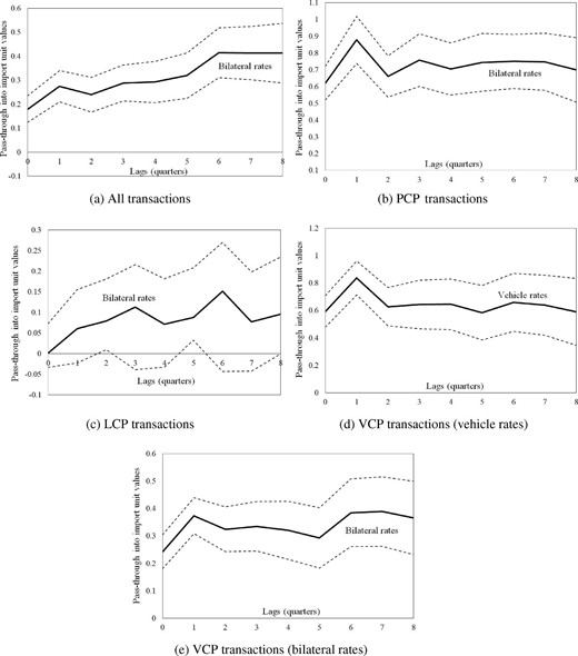
Cumulative pass-through into import unit values. (a) All transactions (based on the estimates of column 1 in Table 5), (b) PCP transactions, (c) LCP transactions, (d) VCP transactions with vehicle rates (based on the estimates of column 4 in Table 5), and (e) VCP transactions with bilateral rates (based on the estimates of column 2 in Table 5). Dashed lines denote 95% confidence intervals. Source: HMRC administrative data sets.
Panels (b)–(d) show the dynamics of pass-through by invoicing choice. They are based on the specification reported in column (4) of Table 5 which lets the unit values in vehicle currencies depend on sterling to vehicle currency exchange rates. For producer currency transactions in panel (b), contemporaneous pass-through is 62.0% and reaches 70.0% after eight quarters (significant at the 1% level). For local currency transactions, panel (c) shows that pass-through increases from zero on impact to 9.6% after two years (the estimate is insignificant, however).
Panel (d) focuses on transactions in vehicle currencies. Pass-through is 59.2% on impact. It remains at essentially the same magnitude after eight quarters (at 59.0% which is significant at the 1% level). Based on bilateral exchange rates (see the estimates reported in column 2 of Table 5), panel (e) shows that pass-through for vehicle currency transactions is only 24.2% on impact, and 36.6% after eight quarters (both significant at the 1% level).
3.3. Reconciling Pass-Through Estimates with the Theoretical Literature
In light of the theoretical literature, we now discuss how the pass-through patterns we find in the data can inform us about the pricing strategies of firms.
As key contributions in the literature, the models of Engel (2006) and Gopinath et al. (2010) demonstrate that when prices are sticky (because of costs to renegotiating prices), firms optimally choose the currency of invoicing in order to keep their preset price closer to their desired price in periods when they do not adjust. If a firm desires low pass-through, it will choose LCP. Conversely, if it desires high pass-through, it will choose PCP.26 As a result, for a given invoicing choice, short-run pass-through should be close to long-run pass-through (as the latter approximates desired pass-through), and the pass-through rates across different invoicing choices should not converge in the long run. Empirically, Gopinath et al. (2010) find that even conditional on a price change, the difference in pass-through into US import prices invoiced in US dollars versus non-US dollars is large even at a two-year horizon.
We argue that our results are consistent with such models where prices are sticky and firms endogenously choose their invoicing currency (Burstein and Gopinath 2014; Engel 2006; Gopinath 2015; Gopinath et al. 2010; Mukhin 2018). First, we find that pass-through is zero for local currency transactions, and large for transactions in foreign currencies. Moreover, pass-through displays dynamics over time. These results are consistent with the assumption that prices are not fully flexible (Gopinath and Itskhoki 2010; Gopinath and Rigobon 2008).27 This can arise because prices are adjusted infrequently in their invoicing currency, and/or because they respond only partially to exchange rate shocks. But as we only observe unit values we are unable to distinguish between the two explanations (i.e., we cannot estimate pass-through conditional on observed price changes). Second, consistent with endogenous invoicing currency pricing, Figure 1 shows that for each invoicing choice there is little difference between short- and long-run pass-through such that the pass-through rates across invoicing choices do not converge in the long run.28,29
Our findings are thus inconsistent with a framework of sticky prices and exogenous invoicing currencies as it predicts that pass-through should be the same across invoicing currencies once prices adjust in the long run (Betts and Devereux 2000; Devereux and Engel 2003; Obstfeld and Rogoff 1995). Neither can our results be explained by models where prices fully adjust every period (Dornbusch 1987; Krugman 1987) as in that case, the currency choice should be irrelevant for pass-through even in the short run. Finally, our results also conflict with models where prices are fixed (Fleming 1962; Mundell 1963). If prices remained rigid in their currency of invoicing (because exporters set a contract price in a given currency and do not adjust this price in response to exchange rate movements), pass-through would be “passive” and only follow mechanically from changes in sterling unit values invoiced in foreign currencies. Contemporaneous pass-through would be zero for local currency transactions, complete for producer and vehicle currency transactions (with respect to vehicle currency exchange rates), and the coefficients on all exchange rate lags would be jointly insignificant. As shown in columns (3) and (4) of Table 5 and in Figure 1, pass-through is large but incomplete for producer and vehicle currency transactions, and we can reject the hypothesis that the coefficients on all exchange rate lags are jointly insignificant (see Online Appendix C for further evidence against the notion of passive pass-through).30
3.4. Robustness and Extensions
Online Appendix D reports a battery of robustness checks, and the patterns we find are supportive of our conclusions. In summary, we run regressions separately on subsamples of import transactions priced in producer, local, and vehicle currencies. We control for changes in the trade-weighted exchange rate to account for strategic complementarities in price setting at the firm level (Gopinath and Itskhoki 2011). We show that our estimates remain similar in magnitude for the period after June 2016 when sterling depreciated following the E.U. referendum. We aggregate our data at monthly and annual frequency. At monthly frequency, we find that the effects of exchange rate changes kick in after one month only. Unit values therefore hardly adjust in the first month following an exchange rate change.
We run regressions using trade values as weights, using the producer price index rather than the consumer price index to control for foreign costs, and excluding homogeneous commodities from the sample. We estimate our regressions separately for manufacturing industries, for the goods produced in the exporting country, for intermediate, final, and capital goods, for differentiated and homogeneous goods (Rauch 1999), and controlling for different modes of transport (sea, rail, road, and air). To account for productivity gains in each country that may shift export prices to all destinations, we use annual frequency data at the six-digit HS level from United Nations Comtrade to control for the growth of each country’s total exports by product category (excluding exports to the United Kingdom). Besides, as our regressions do not include product-specific variables, we experiment with different combinations of product fixed effects (country-product-year, country-product-quarter, product-quarter, and firm-country-product fixed effects). We distinguish between firms based on their average import shares. We exclude from our sample the United States, China, and the countries with fixed exchange rate regimes, crawling pegs, and with pegs to the US dollar or the euro. We demonstrate that our results remain robust to alternative combinations of firm-quarter and origin-product fixed effects. Finally, we show that pass-through remains heterogeneous across invoicing choices when we identify the effects of bilateral exchange rate changes on the unit values of firms importing a given product from a given country using different invoicing currencies.
Online Appendix E reports results for export unit values. The pass-through of bilateral exchange rate changes into export unit values is zero for the transactions in producer and vehicle currencies, and large for the ones in local currencies. The export unit values of vehicle currency transactions react to changes in the sterling to vehicle currency exchange rate, but not to changes in the vehicle to destination country’s currency exchange rate. Online Appendix F shows that regardless of the currency of invoicing, export and import quantities only react modestly, if at all, to changes in exchange rates.
3.5. VCP and Dominant Currency Paradigm
We now explain how our approach that emphasizes vehicle currencies differs from, and compares to, the Dominant Currency Paradigm that stresses the importance of dominant currencies such as the US dollar in explaining pass-through (Gopinath 2015; Gopinath et al. 2020).
First, although they both imply that bilateral exchange rates are inappropriate in pass-through regressions, DCP and VCP are conceptually different. In contrast to DCP, VCP distinguishes between the US dollar as a producer currency and a vehicle currency. Moreover, it considers other vehicle currencies than the US dollar in explaining pass-through. There is, however, a strong overlap between DCP and VCP because the US dollar, which is the dominant currency, is also the main vehicle currency. Thanks to the availability of bilateral currency of invoicing data between the United Kingdom and its non-E.U. trading partners (as opposed to aggregate country-level data), we are indeed able to document that 88.5% of vehicle currency transactions in our sample are invoiced in US dollars, 10.9% in euros, and 0.6% in 89 other currencies.
To establish whether the differences between DCP and VCP matter for pass-through, we estimate pass-through separately for vehicle currency transactions in US dollars and non-US dollars. In column (1) of Table 7, we run the specification of column (4) in Table 5 but interact the vehicle currency exchange rates with dummy variables for the US dollar and non-US dollar currencies. As the coefficients on the two vehicle currency exchange rates are not significantly different from each other, pass-through is the same whether the vehicle currency is the US dollar or another currency. It is therefore the use of vehicle currencies generally, and not the US dollar specifically, that is driving the high pass-through for vehicle currency transactions. Non-US dollar vehicle currencies are far less pervasive than the US dollar, but our contribution is to show that they also matter for pass-through. This finding could be seen as extending the results of Gopinath et al. (2020) to vehicle currencies less prominent than the US dollar.31
Pass-through for US dollar versus non-US dollar currencies.
| (1) | (2) | |
|---|---|---|
| Δln e|${{ij,\!t}}$| × DPCP | |$\underset{\left( 0.050\right) }{0.631}$|*** | – |
| |$\Delta \ln e_{ij,t}\times D_{\rm {PCP}}\times D_{\vn {USD}}$| | – | |$\underset{\left( 0.069\right) }{0.624}$|*** |
| |$\Delta \ln e_{ij,t}\times D_{\rm {PCP}}\times D_{\vn {non-USD}}$| | – | |$\underset{\left( 0.053\right) }{0.617}$|*** |
| Δln e|${{ij,\!t}}$| × DLCP | |$\underset{\left( 0.036\right) }{0.013}$| | |$\underset{\left( 0.037\right) }{0.014}$| |
| |$\Delta \ln e_{iV,t}\times D_{ \rm {VCP}}\times D_{\vn {USD}}$| | |$\underset{\left( 0.105\right) }{0.483}$|*** | |$\underset{\left( 0.106\right) }{0.488}$|*** |
| |$\Delta \ln e_{iV,t}\times D_{ \rm {VCP}}\times D_{\vn {non-USD}}$| | |$\underset{\left( 0.059\right) }{0.591}$|*** | |$\underset{\left( 0.061\right) }{0.590}$|*** |
| Firm-quarter fixed effects | Yes | Yes |
| Origin-product fixed effects | Yes | Yes |
| Invoicing choice fixed effects | Yes | Yes |
| USD dummy | Yes | Yes |
| Observations | 5,212,592 | 5,212,592 |
| R-squared | 0.146 | 0.146 |
Notes. Contemporaneous and eight lags of the origin country’s quarterly inflation rate, as well as eight lags of the log change in each exchange rate are also included (not reported). Robust standard errors adjusted for clustering at the country-year level are reported in parentheses. *** indicates significance at the 1% level. The dependent variable is the quarterly log change import unit value (in sterling per kilogram). Source: HMRC administrative data sets.
Next, in column (2), we also let the coefficient on the bilateral exchange rate for producer currency transactions vary between the US dollar and other currencies. As we cannot reject the hypothesis that the coefficients on the two vehicle currency exchange rates and the two bilateral exchange rates are equal, we conclude that pass-through is high and of the same magnitude for vehicle and producer currency transactions, regardless of whether the invoicing currency is the US dollar or another currency.
Overall, our results in Table 7 demonstrate that the behavior of exchange rate pass-through is consistent with the predictions of both DCP and VCP. On one hand, as the US dollar is a dominant currency, its pass-through is high and of the same magnitude regardless of whether it is used as a producer or a vehicle currency. On the other hand, pass-through is equally high for vehicle currency transactions in US dollars and non-US dollars.
Second, Gopinath et al. (2020) find that the pass-through of the euro exchange rate is negligible compared to the pass-through of the US dollar exchange rate. For the UK economy, we instead expect the euro exchange rate to matter in explaining import unit values (in our sample of non-E.U. countries, the euro is mainly used as a vehicle currency).32 In our data set, 10.95% of vehicle currency transactions are priced in euros. Moreover, we observe 36 countries with a euro vehicle currency share for imports to the United Kingdom that is larger than 30% (in fact, 21 countries have a share above 70%). As shown in Table 8, these countries include small trading partners of the United Kingdom such as Bosnia and Herzegovina, Haiti, Croatia, Serbia, and Armenia but also larger partners such as Turkey, Japan, and South Korea.33
Vehicle currency import shares in euros 2010–2017.
| Origin country | VCP import share | Percentage in euros | Non-E.U. import share |
|---|---|---|---|
| Largest euro VCP shares | |||
| Bosnia and Herzegovina | 78.12 | 99.06 | 0.01 |
| Haiti | 100.00 | 98.19 | 0.01 |
| Croatia | 52.21 | 95.32 | 0.02 |
| Serbia | 74.85 | 94.94 | 0.07 |
| Armenia | 57.34 | 91.66 | 0.01 |
| Large euro VCP shares (selected countries) | |||
| Morocco | 58.08 | 89.58 | 0.28 |
| Senegal | 82.96 | 83.79 | 0.01 |
| Turkey | 40.22 | 70.05 | 3.76 |
| Japan | 32.59 | 47.39 | 5.51 |
| South Korea | 40.05 | 32.97 | 2.35 |
Notes. The table reports the vehicle currency import share of the United Kingdom from each country for 2010–2017, its share in euros, and the share of each country in the United Kingdom total non-E.U. imports (all in %). Countries ordered by decreasing euro VCP share (second column). Source: HMRC administrative data sets.
We first report in column (1) of Table 9 the results of estimating equation (4) with bilateral exchange rates only. Pass-through is equal to 44.6%, which is larger than the 17.9% we obtain with firm-quarter fixed effects (column 1 of Table 5). In column (2), we further control for the US dollar exchange rate. Consistent with Gopinath et al. (2020), the pass-through of the US dollar exchange rate is relatively large at 40.1%, while the coefficient on the bilateral exchange rate shrinks from 0.446 to 0.247. In column (3), we add the euro exchange rate.34 The US dollar pass-through rate increases to 60.4%, and the coefficient on the bilateral exchange rate further falls to 0.234. The pass-through of the euro exchange rate is 26.6%, which is only slightly larger than the pass-through of the bilateral exchange rate.35
Pass-through for dominant currencies (US dollar and euro).
| (1) | (2) | (3) | (4) | (5) | (6) | |
|---|---|---|---|---|---|---|
| Δln e|${{ij,\!t}}$| | |$\underset{\left( 0.037\right) }{0.446}$|*** | |$\underset{\left( 0.028\right) }{0.247}$|*** | |$\underset{\left( 0.028\right) }{0.234}$|*** | – | – | – |
| Δln ei $,t | – | |$\underset{\left( 0.037\right) }{0.401}$|*** | |$\underset{\left( 0.059\right) }{0.604}$|*** | – | – | – |
| |$\Delta \ln e_{i\euro ,t}$| | – | – | |$\underset{\left( 0.048\right) }{0.266}$|*** | – | – | – |
| Δln e|${{ij,\!t}}$| × DPCP | – | – | – | |$\underset{\left( 0.043\right) }{0.703}$|*** | |$\underset{\left( 0.059\right) }{0.781}$|*** | |$\underset{\left( 0.041\right) }{0.735}$|*** |
| Δln ei $,t × DPCP | – | – | – | – | |$\underset{\left( 0.101\right) }{0.154}$| | – |
| |$\Delta \ln e_{i\euro ,t}\times D_{\rm {PCP}}$| | – | – | – | – | |$\underset{\left( 0.059\right) }{0.300}$|*** | – |
| Δln e|${{ij,\!t}}$| × DLCP | – | – | – | |$\underset{\left( 0.026\right) }{0.130}$|*** | |$\underset{\left( 0.029\right) }{0.109}$|*** | |$\underset{\left( 0.024\right) }{0.122}$|*** |
| Δln ei $,t × DLCP | – | – | – | – | |$\underset{\left( 0.073\right) }{0.374}$|*** | – |
| |$\Delta \ln e_{i\euro ,t}\times D_{\rm {LCP}}$| | – | – | – | – | |$\underset{\left( 0.049\right) }{0.167}$|*** | – |
| |$\Delta \ln e_{ij,t}\times D_{ \rm {VCP}}$| | – | – | – | |$\underset{\left( 0.050\right) }{0.499}$|*** | |$\underset{\left( 0.028\right) }{0.144}$|*** | – |
| |$\Delta \ln e_{i\$,t}\times D_{ \rm {VCP}}$| | – | – | – | – | |$\underset{\left( 0.060\right) }{0.756}$|*** | – |
| |$\Delta \ln e_{{i\euro},t}\times D_{ \rm {VCP}}$| | – | – | – | – | |$\underset{\left( 0.057\right) }{0.341}$|*** | – |
| |$\Delta \ln e_{iV,t}\times D_{ \rm {VCP}}$| | – | – | – | – | – | |$\underset{\left( 0.028\right) }{0.707}$|*** |
| Firm-year fixed effects | Yes | Yes | Yes | Yes | Yes | Yes |
| Origin-product fixed effects | Yes | Yes | Yes | Yes | Yes | Yes |
| Invoicing choice fixed effects | No | No | No | Yes | Yes | Yes |
| Observations | 5,674,778 | 5,674,778 | 5,674,778 | 5,674,778 | 5,674,778 | 5,674,778 |
| R-squared | 0.051 | 0.051 | 0.051 | 0.051 | 0.051 | 0.051 |
Notes. Contemporaneous and eight lags of the origin country’s quarterly inflation rate, as well as eight lags of the log change in each exchange rate are also included (not reported). Robust standard errors adjusted for clustering at the country-year level are reported in parentheses. *** indicates significance at the 1% level. The dependent variable is the quarterly log change import unit value (in sterling per kilogram). Source: HMRC administrative data sets.
The importance of the euro in explaining UK import unit values becomes clearer in columns (4) and (5). They report the same specifications as in columns (1) and (3) but all exchange rates are further interacted with dummy variables for each invoicing choice. Compared to column (4), column (5) shows that controlling for the US dollar and euro exchange rates significantly reduces the magnitude of the coefficient on the bilateral exchange rate but for vehicle currency transactions only (to 0.144 from 0.499). This confirms that bilateral exchange rates are unsuitable for explaining import unit values invoiced in vehicle currencies. Instead, for producer and local currency transactions, controlling for the US dollar and euro exchange rates leaves the coefficients on the bilateral exchange rate mostly unchanged. For these transactions, the bilateral exchange rate therefore does a good job at explaining import unit values.
For vehicle currency transactions, the pass-through of the US dollar exchange rate is high at 75.6%, capturing the fact that the US dollar is widely used as a vehicle currency. The pass-through of the euro exchange rate is lower at 34.1%, but it is twice as large as the pass-through of the bilateral exchange rate. These results provide evidence that in addition to the US dollar exchange rate, the euro exchange rate also contributes to explaining UK import unit values invoiced in vehicle currencies.
Given that most data sets do not disaggregate trade data by currency of invoicing, how can researchers address the low pass-through estimates that arise from not accounting for invoicing choices? Without currency of invoicing information, researchers can only estimate columns (1)–(3) of Table 9. As the US dollar and to some extent the euro exchange rates have a larger impact on import unit values than the bilateral exchange rate, controlling for the two exchange rates helps to increase pass-through estimates. But by how much? Column (6) reports our baseline specification of column (4) in Table 5 but with firm-year fixed effects. Pass-through is large at 73.5% and 70.7% for producer and vehicle currency transactions, and low at 12.2% for local currency transactions. The pass-through rates for producer and vehicle currency transactions are thus larger than the ones we obtain in column (3) for the US dollar and euro exchange rates. In other words, although the US dollar and euro exchange rates help to increase pass-through estimates, they fall short of replicating the magnitude of our pass-through elasticities based on actual invoicing currencies.
4. Implications for Import Price Inflation
Our results demonstrate that pass-through is higher once we let the unit values invoiced in vehicle currencies depend on vehicle currency exchange rates. As changes in import prices feed into consumer prices, our results imply that pass-through into consumer prices should also be higher once we account for vehicle currency exchange rates. Pass-through into consumer prices is, however, typically lower than into import prices because consumer prices contain a larger non-traded component due to local distribution costs, and they include the prices of non-tradable and tradable goods and services only sold domestically (Bacchetta and van Wincoop 2003; Burstein and Gopinath 2014; Campa and Goldberg 2010; Gopinath 2015).36
To derive the implications of our results for consumer price inflation, we would need to match import unit values with the microdata underlying the construction of the UK consumer price index (Auer et al. 2021). These data, however, are not available by invoicing currency. We therefore focus our analysis on import price inflation, assuming the patterns we find for import unit values are transmitted to consumer prices. As shown in Figure 2, the year-on-year monthly import and consumer price inflation rates between January 2007 and August 2018 are indeed highly correlated (the correlation is 77%), although the import price index is more volatile than the consumer price index (the year-on-year monthly percentage change varies between −7.96 and 18.42 for import prices, and between 0.20 and 4.79 for consumer prices). As the import component of the UK consumer price index is around 30% (Forbes et al. 2018), the effects of exchange rate changes on consumer price inflation should amount to roughly one-third of the effects we report for import price inflation (Gopinath 2015).
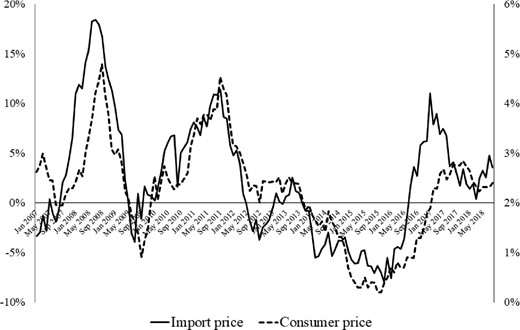
Consumer (right axis) and import (left axis) price inflation for the UK economy (% change over 12 months) from January 2007 to August 2018. Source: International Financial Statistics of the International Monetary Fund.
To illustrate how exchange rate movements affect import price inflation in the short run (i.e., within one quarter) and in the long run (i.e., after eight quarters), we focus on three quarterly episodes of large sterling fluctuations. First, following the E.U. referendum, sterling depreciated in June–August 2016 (relative to the previous March–May 2016 quarter) by 7.09% on average (on a trade-weighted basis), and by 6.34% and 7.66% against the US dollar and the euro, respectively. Second, during the Great Recession sterling depreciated in November 2008–January 2009 by 12.94% on average, and by 19.43% and 12.34% against the US dollar and the euro, respectively. Finally, in the aftermath of the European Sovereign Debt Crisis, sterling appreciated in January–March 2015 by 2.66% and 6.24% on average and against the euro but depreciated by 4.76% against the US dollar.37 Figure 3 plots the monthly nominal sterling exchange rates against the euro and the US dollar from January 2007 to August 2018, as well as the nominal effective exchange rate. The vertical shaded areas indicate the three quarterly episodes of sterling fluctuations we focus on.
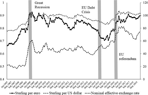
Sterling per euro and sterling per US dollar nominal exchange rates (left axis), and nominal effective sterling exchange rate index (right axis) from January 2007 to August 2018. Source: International Financial Statistics of the International Monetary Fund.
To calculate our back-of-the-envelope estimates, we proceed as follows (for full details, see Online Appendix G).38 First, as our data set provides the invoicing currency for non-E.U. imports only, we combine it with data from Gopinath (2015) to derive the invoicing shares for UK world imports. Due to data limitations, we consider two alternative scenarios for the magnitude of these shares (scenarios 1 and 2, see Online Appendix Table G1). Second, for each of the three episodes, we measure the change of all exchange rates in the quarter of the shock relative to the previous quarter. We then calculate weighted averages by weighting the bilateral exchange rate changes with bilateral import shares in local and producer currencies, and the vehicle currency exchange rate changes with each vehicle currency’s import share. Third, based on the estimates of column (4) in Table 5, for each invoicing choice we evaluate the effects of these weighted exchange rate changes on import price inflation, and we aggregate them using the invoicing shares for world imports.39 As a comparison, based on the estimates of column (1) in Table 5, we also derive predictions that do not account for invoicing currencies and only capture the effects of bilateral exchange rate changes (weighted by bilateral import shares). In this section, we present results for world imports based on scenario 1 for the invoicing shares.40 The results for scenario 2 (and for non-E.U. imports) are relegated to Online Appendix Table G2. They are qualitatively similar to the ones we report below.
We start with the depreciation of sterling following the E.U. referendum of June 2016. We present our estimates in columns (1) and (2) of Table 10. Column (1) shows that when we consider the effects of bilateral exchange rates only, the average (trade-weighted) depreciation of sterling increases import price inflation by 1.271 percentage points on impact. After eight quarters, inflation rises by 2.927 percentage points (column 2). The next two rows report the individual contributions of the US dollar and the euro. The depreciation against the euro increases import price inflation by more than the depreciation against the US dollar. The reason is that a large share (49.95%) of UK imports originates from the E.U. The depreciation against the euro is therefore given a larger weight than the depreciation against the US dollar in driving import price inflation.
The effects of exchange rate shocks on UK import price inflation.
| (1) | (2) | (3) | (4) | (5) | (6) | ||||||
|---|---|---|---|---|---|---|---|---|---|---|---|
| E.U. referendum | Great Recession | E.U. Debt Crisis | |||||||||
| Exchange rates | Currencies | t = 0 | t = 8 | t = 0 | t = 8 | t = 0 | t = 8 | ||||
| Bilateral | All | |$\underset{\left( 0.199\right) }{1.271}$|*** | |$\underset{\left( 0.447\right) }{2.927}$|*** | |$\underset{\left( 0.363\right) }{2.321}$|*** | |$\underset{\left( 0.815\right) }{5.343}$|*** | |$\hphantom{00}\underset{\left( 0.075\right) }{-0.477}$|*** | |$\underset{\hphantom{0}\left( 0.167\right) }{-1.098}$|*** | ||||
| USD | |$\underset{\left( 0.016\right) }{0.105}$|*** | |$\underset{\left( 0.037\right) }{0.243}$|*** | |$\underset{\left( 0.050\right) }{0.323}$|*** | |$\underset{\left( 0.113\right) }{0.744}$|*** | |$\underset{\left( 0.012\right) }{0.079}$|*** | |$\underset{\left( 0.028\right) }{0.182}$|*** | |||||
| Euro | |$\underset{\left( 0.104\right) }{0.668}$|*** | |$\underset{\left( 0.235\right) }{1.537}$|*** | |$\underset{\left( 0.168\right) }{1.076}$|*** | |$\underset{\left( 0.378\right) }{2.477}$|*** | |$\underset{\hphantom{0}\left( 0.085\right) }{-0.544}$|*** | |$\underset{\hphantom{0}\left( 0.191\right) }{-1.252}$|*** | |||||
| Bilateral/vehicle | All | |$\underset{\left( 0.283\right) }{2.788}$|*** | |$\underset{\left( 0.609\right) }{3.157}$|*** | |$\underset{\left( 0.690\right) }{7.100}$|*** | |$\underset{\left( 1.489\right) }{7.772}$|*** | |$\underset{\left( 0.076\right) }{0.619}$|*** | |$\underset{\left( 0.146\right) }{0.466}$|*** | ||||
| USD | |$\underset{\left( 0.162\right) }{1.775}$|*** | |$\underset{\left( 0.348\right) }{1.812}$|*** | |$\underset{\left( 0.497\right) }{5.435}$|*** | |$\underset{\left( 1.065\right) }{5.550}$|*** | |$\underset{\left( 0.122\right) }{1.330}$|*** | |$\underset{\left( 0.261\right) }{1.358}$|*** | |||||
| Euro | |$\underset{\left( 0.105\right) }{0.876}$|*** | |$\underset{\left( 0.217\right) }{1.113}$|*** | |$\underset{\left( 0.169\right) }{1.411}$|*** | |$\underset{\left( 0.350\right) }{1.793}$|*** | |$\underset{\hphantom{0}\left( 0.085\right) }{-0.713}$|*** | |$\underset{\hphantom{0}\left( 0.177\right) }{-0.906}$|*** | |||||
| Exchange rate shock | 2016M6–2016M8 | 2008M11–2009M1 | 2015M1–2015M3 | ||||||||
| Sterling (trade-weighted) | +7.09% | +12.94% | −2.66% | ||||||||
| Sterling against US dollar | +6.34% | +19.43% | +4.76% | ||||||||
| Sterling against euro | +7.66% | +12.34% | −6.24% | ||||||||
Notes. The estimates show changes in UK import price inflation, reported in percentage points. The estimates reported in the rows “Bilateral” are obtained based on the regression in column (1) of Table 5. The estimates reported in the rows “Bilateral/vehicle” are obtained using the regression in column (4) of Table 5. *** indicates significance at the 1% level. Source: HMRC administrative data sets.
Once we account for the full breadth of invoicing currencies and relevant pass-through estimates, our results yield much larger effects on import price inflation. Columns (1) and (2) of Table 10 show that the depreciation of sterling increases import price inflation by 2.788 percentage points on impact, and by 3.157 percentage points after eight quarters. The reason for the bigger estimates is that the pass-through of vehicle currency exchange rates into import unit values in vehicle currencies is large. As the US dollar is used extensively as a vehicle currency, the depreciation against the US dollar is therefore given a larger weight in affecting import prices (it increases import price inflation by 1.775 percentage points on impact and 1.812 percentage points after two years). This finding is consistent with Gopinath et al. (2020) who argue that countries with larger US dollar import invoicing shares experience higher pass-through of US dollar exchange rate changes into consumer price inflation.
Columns (3) and (4) report our results for the Great Recession. Similarly to the E.U. referendum, we find that the depreciation of sterling has a larger inflationary impact once we let unit values in vehicle currencies depend on vehicle currency exchange rates. The higher import price inflation is again driven by the US dollar as it is mainly used as a vehicle currency.
Columns (5) and (6) focus on the European Sovereign Debt Crisis. When we only consider the effects of bilateral exchange rates, the average appreciation of sterling reduces import price inflation in the short and long runs. Due to the intensity of trade between the United Kingdom and the E.U., the fall in import price inflation is driven by the appreciation against the euro, which outweighs the effect of the depreciation against the US dollar. But once we account for invoicing choices and for the effects of vehicle currency exchange rates, movements in sterling increase import price inflation in the short and long runs. The reason is that the depreciation against the US dollar now outweighs the appreciation against the euro in affecting import unit values. The European Sovereign Debt Crisis is thus an example where accounting for invoicing choices does not only matter quantitatively but also qualitatively.
Panels (a)–(c) of Figure 4 depict the dynamics of each exchange rate shock. Once we account for invoicing currencies, the depreciation of sterling increases inflation to a larger extent after the E.U. referendum and during the Great Recession (panels a and b). For the European Sovereign Debt Crisis, the fall in inflation induced by the appreciation against the euro is more than offset by the depreciation against the US dollar (panel c).
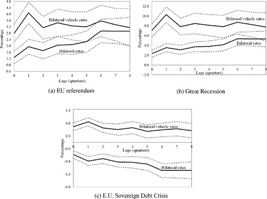
Solid lines plot the cumulative effects of sterling exchange rate shocks on import price inflation: (a) after the E.U. referendum, (b) during the Great Recession, and (c) after the E.U. Sovereign Debt Crisis. The “Bilateral rates” estimates are obtained based on the regression in column (1) of Table 5, while the “Bilateral/vehicle rates” estimates are obtained based on column (4) of Table 5. Dashed lines denote 95% confidence intervals. Source: HMRC administrative data sets.
As further evidence that accounting for vehicle currencies results in more accurate predictions of exchange rate effects on import price inflation, in Online Appendix G we perform an out-of-sample prediction of UK import unit values. We recalculate our back-of-the-envelope estimates for the depreciation of sterling following the E.U. referendum based on pre-referendum invoicing shares and pass-through elasticities (reported in Online Appendix Table D3). On impact, import price inflation rises by 1.367 percentage points based on bilateral exchange rates, and by 2.933 percentage points once we account for vehicle currency exchange rates (see Online Appendix Table G4). Actual import price inflation (relative to the previous quarter) rose from 1.108% in March–May 2016 to 3.767% in June–August 2016, or a 2.659 percentage point increase. Our prediction involving invoicing currencies therefore does a good job at matching the data while the prediction based on bilateral exchange rates is less accurate.
To conclude, once we account for invoicing currencies, we can explain why pass-through into import unit values was higher than expected during the Great Recession and after the E.U. referendum, and lower than expected in the aftermath of the European Sovereign Debt Crisis. The reason is that for transactions in vehicle currencies, import unit values respond more to changes in the vehicle currency exchange rate than in the bilateral exchange rate.
5. Discussion: Exchange Rate Disconnect
Our estimates from previous sections show that exchange rate pass-through is substantially higher once we account for vehicle currencies. To better understand this finding, we present a simple conceptual framework to interpret our pass-through estimates. We hope our discussion can help to explain why researchers often find a weak relationship, or “disconnect”, between exchange rates and prices when not accounting for vehicle currencies.41
As columns (1) and (2) of Table 5 show, the low pass-through coefficient on bilateral exchange rates is partly due to a lacking distinction between producer currency and local currency transactions. Once we make that distinction in column (2), the pass-through coefficient increases. That point is well understood in the literature. In the following, instead, we zoom in on vehicle currency transactions. As we show in Table 2, those are by a substantial margin the most prevalent UK import transactions, and this context is where our results from previous sections provided new empirical insights.
As a simple conceptual framework, we outline a three-country model of exchange rate pass-through under VCP. Figure 5 illustrates the setting. Monopolistic exporters are based in foreign country j and sell to the domestic country i (the United Kingdom). They set the price in a third-country currency, that is, they invoice in a vehicle currency V. This is an extension of the two-country model in Engel (2006) that does not feature a vehicle currency. As in Engel (2006), we assume firms determine a price-setting function in advance such that they retain an element of flexibility and prices are not necessarily sticky. In particular, firms can commit to setting their prices as a log-linear function of the exchange rate. That is, firms index their prices to the exchange rate, and they optimally choose the pass-through rate. Intuitively, firms form an “optimal linear forecast”.42
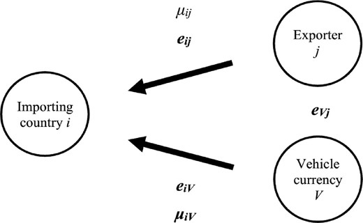
This figure illustrates the relationship between exporters in country j shipping to country i and the vehicle currency. Firms set prices in the vehicle currency. They either react to the bilateral exchange rate eij or the vehicle currency exchange rate eiV, as indicated by the arrows, where μij and μiV refer to corresponding pass-through elasticities in equations (5) and (6). Triangular arbitrage holds for exchange rates such that ln eij = ln eiV + ln eVj as in equation (2).
where |$\Delta \ln p_{V}^{ij}$| denotes the change of the log vehicle currency price set by firms who react to the bilateral exchange rate, and |$\Delta \ln p_{V}^{iV}$| is the log vehicle currency price change for firms who react to the vehicle currency exchange rate.43 The coefficients μ|${{ij}}$| and μ|${{iV}}$| are the corresponding pass-through elasticities into vehicle currency prices, chosen optimally by firms. For example, suppose sterling depreciates against the vehicle currency (Δln e|${{iV}}$| > 0). For μ|${{iV}}$| = 0, the vehicle currency price |$p_{V}^{iV}$| would be unresponsive. More realistically, we would typically expect firms to respond by lowering the vehicle currency price, implying μ|${{iV}}$| < 0. We refer to Online Appendix H for derivations and further details as those are not essential for our argument here.
In Table 11, we estimate specification (9) for the subsample of vehicle currency transactions. As in regressions from previous sections, we include exchange rate lags, inflation rates, and fixed effects, and we report the contemporaneous coefficients. We highlight three aspects.
Pass-through into import unit values for the VCP subsample.
| (1) | (2) | (3) | (4) | (5) | |
|---|---|---|---|---|---|
| Δln e|${{ij,\!t}}$| | |$\underset{\left( 0.035\right) }{0.094}$|*** | |$\underset{\left( 0.033\right) }{0.123}$|*** | – | |$\underset{\left( 0.149\right) }{0.612}$|*** | – |
| Δln e|${{iV\!,\!t}}$| | |$\underset{\left( 0.158\right) }{0.518}$|*** | – | |$\underset{\left( 0.155\right) }{0.535}$|*** | – | |$\underset{\left( 0.149\right) }{0.612}$|*** |
| Δln e|${{Vj,\!t}}$| | – | – | – | |$\underset{\left( 0.158\right) }{-0.518}$|*** | |$\underset{\left( 0.035\right) }{0.094}$|*** |
| Firm-quarter fixed effects | Yes | Yes | Yes | Yes | Yes |
| Origin-product fixed effects | Yes | Yes | Yes | Yes | Yes |
| Observations | 2,599,543 | 2,599,543 | 2,599,543 | 2,599,543 | 2,599,543 |
| R-squared | 0.176 | 0.176 | 0.176 | 0.176 | 0.176 |
Notes. Contemporaneous and eight lags of the origin country’s quarterly inflation rate, as well as eight lags of the log change in each exchange rate are also included (not reported). Robust standard errors adjusted for clustering at the country-year level are reported in parentheses. *** indicates significance at the 1% level. The dependent variable is the quarterly log change import unit value (in sterling per kilogram). Source: HMRC administrative data sets.
First, the results in column (1) show that the vehicle currency exchange rate displays substantially higher pass-through (ϕ2 = 0.518) than the bilateral exchange rate (ϕ1 = 0.094), and the two coefficients are significantly different from each other. This means that in the aggregate, sterling prices adjust by about 50% of a vehicle currency exchange rate movement, but only by about 10% of a bilateral exchange rate movement.45 Bilateral exchange rates therefore hardly matter for pass-through. But since pass-through is rather strong with respect to vehicle currency exchange rates, it would be misleading to describe the overall results as exchange rate disconnect.
Second, as we show in columns (2) and (3), the pass-through coefficients hardly change when estimated in isolation. Thus, there is no obvious omitted variable bias when we drop one of the exchange rate regressors. We stress that we obtain this result only when we are able to separately identify vehicle currency transactions as in Table 11. As we show in Table 9, this result does not hold once they are pooled with producer currency and local currency transactions.46
In summary, although specifications (10) and (11) are equivalent due to triangular arbitrage, specification (9) highlights the contrast between bilateral and vehicle currency exchange rate pass-through most succinctly. Our framework suggests researchers should ideally include two exchange rate variables in pass-through regressions to account for vehicle currency transactions. Various alternatives are possible. But when only controlling for the bilateral exchange rate, researchers would find a low pass-through coefficient in the presence of vehicle currency transactions. They should not erroneously interpret this finding as exchange rate disconnect.
6. Concluding Remarks
Using detailed firm-level transactions data for UK imports from non-E.U. countries, we establish that invoicing in a vehicle currency is pervasive. We then examine the relationship between the currency of invoicing and exchange rate pass-through. Pass-through varies substantially across invoicing choices. It is large for imports invoiced in producer currencies but insignificant for invoicing in local currency (sterling). Once we let import unit values invoiced in vehicle currencies depend on the vehicle currency exchange rate rather than the bilateral exchange rate, pass-through is large and in the same ballpark as for PCP. Taking vehicle currencies into account therefore raises estimated exchange rate pass-through. Overall, our results help to explain why the literature often finds a disconnect between exchange rates and prices when failing to account for vehicle currencies.
For policy purposes, our results imply that ignoring the currency of invoicing can produce misleading predictions regarding exchange rate pass-through into import prices and therefore also consumer prices. Policymakers should take into account that when VCP is pervasive, bilateral exchange rates are inappropriate for determining the impact of exchange rate changes on prices. They should construct an effective nominal exchange rate that is based on invoicing currency weights, not trade weights.
Notes
The editor in charge of this paper was Claudio Michelacci.
Acknowledgments
We are grateful to the editor Claudio Michelacci and to four anonymous referees for many valuable comments. We are grateful for financial support from the Bank of England Research Donations Committee, Grant RDC201615. Any views expressed are solely those of the authors and cannot be taken to represent those of the Bank of England or to state Bank of England policy. We are also grateful for financial support from the Birmingham Business School Research and Knowledge Transfer Committee, the Centre for Competitive Advantage in the Global Economy (CAGE, ESRC grant ES/L011719/1) at the University of Warwick, and the Economic and Social Research Council (ESRC grant ES/P00766X/1). We would like to thank Andrew Bernard, Meredith Crowley, Oleg Itskhoki, John Lewis, Katrin Rabitsch, Jeremy Smith, Walter Steingress, Gregory Thwaites, Cédric Tille, Ben Tomlin, and Robert Zymek. Chen and Novy are CEPR Research Fellows. Chung is a CEPR Research Affiliate.
Disclaimer: This work contains statistical data from HMRC which is Crown Copyright. The research data sets used may not exactly reproduce HMRC aggregates. The use of HMRC statistical data in this work does not imply the endorsement of HMRC in relation to the interpretation or analysis of the information. HMRC agrees that the figures and descriptions of results in the attached document may be published. This does not imply HMRC’s acceptance of the validity of the methods used to obtain these figures, or of any analysis of the results.
Footnotes
For instance, Obstfeld and Rogoff (1995) assume PCP, Betts and Devereux (2000) consider LCP, while Devereux and Engel (2003) allow for both types of invoicing choices. Other factors that may lead to incomplete pass-through include the pricing-to-market behavior of exporters when they differentially adjust their markups across destinations in response to exchange rate changes (Knetter 1989, 1993; Krugman 1987), or the presence of local distribution costs in the destination market (Burstein, Neves, and Rebelo 2003; Corsetti and Dedola 2005).
The data set also provides the universe of the United Kingdom's Free on Board export transactions for which the currency of invoicing is reported from 2011 to 2017 for non-E.U. transactions only. In contrast to imports, the value share of exports is the largest at 53.83% in the producer’s currency (sterling), followed by 23.99% in vehicle currency, and 22.18% in local currency. Online Appendix E shows that our results also apply to export unit values.
See the Bank of England’s inflation reports of May 2009 and August 2015.
The Bank of England uses the Central Organizing Model for Projection Analysis and Scenario Simulation (COMPASS) to forecast future inflation. The model only considers an aggregate exchange rate index and does not allow for currency of invoicing effects. See https://www.bankofengland.co.uk/working-paper/2013/the-boes-forecasting-platform-compass-maps-ease-and-the-suite-of-models. Georgiadis and Mösle (2019) introduce US dollar pricing into ECB–Global, the European Central Bank’s macroeconomic model for the global economy. But they do not investigate the implications of US dollar pricing for inflation forecasts.
A number of recent papers estimate pass-through using firm- or product-level data. See Amiti, Itskhoki, and Konings (2014), Auer and Schoenle (2016), Berman, Martin, and Mayer (2012), Chen and Juvenal (2016), Fitzgerald and Haller (2014), Gopinath and Itskhoki (2010), Gopinath and Rigobon (2008), and Nakamura and Zerom (2010), among others. Mumtaz, Oomen, and Wang (2011) study pass-through into UK import prices using data at the industry level.
A large body of the literature on currency of invoicing and pass-through is theoretical. Engel (2006) and Gopinath et al. (2010) develop models where a firm’s desired pass-through determines the currency of invoicing. In Bacchetta and van Wincoop (2003), currency choice explains why pass-through is lower into consumer than into import prices. Corsetti and Pesenti (2005) study optimal monetary policy in open economies and link the degree of pass-through to the invoicing currency. Also see Choudhri and Hakura (2012) and Devereux, Engel, and Storgaard (2004).
Also see Devereux, Dong, and Tomlin (2017) who show that the market shares of both exporting and importing firms impact exchange rate pass-through and the currency of invoicing.
In our analysis, we take the invoicing choice as given as our aim is not to explain the invoicing strategies of firms. A number of studies investigate the factors that influence invoicing currency choices. Goldberg and Tille (2008) provide evidence that country size matters, whereas hedging considerations and transaction costs play a minor role. Goldberg and Tille (2016) conclude that the invoicing choice results from a bargaining process between trading partners. Lyonnet, Martin, and Méjean (2016) document that exporters using financial instruments to hedge against exchange rate risk are more likely to price in a foreign currency. Chung (2016) shows that UK exporters relying on foreign currency-denominated imported inputs are less likely to invoice in their home currency. See also Donnenfeld and Haug (2003), Friberg and Wilander (2008), Ito, Koibuchi, Sato, and Shimizu (2010, 2013, 2016), Kamps (2006), and Ligthart and Werner (2012). For models investigating the determinants of currency choice, see Bacchetta and van Wincoop (2005), Devereux et al. (2017), Engel (2006), Friberg (1998), Goldberg and Tille (2008), Gopinath et al. (2010), Gopinath and Stein (2021), and Mukhin (2018).
In general, the currency of invoice and the currency of settlement are the same (Friberg and Wilander 2008).
Alternatively, unit values can be measured per unit as opposed to per kilogram. In results available upon request, we show that our findings remain very similar although the sample size is smaller.
We are thus unable to estimate pass-through conditional on an observed price change (Gopinath and Rigobon 2008). Another issue is that approximating prices using unit values for aggregated product categories (in our case, at the ten-digit level) may conflate price changes with changes in the composition or quality of traded goods. To address the issue of quality heterogeneity, we calculate the number of transport modes by firm-product-country (sea, rail, road, and air), and in columns (8) and (9) of Online Appendix Table D8, we split our sample between the triplets with one or more than one transport modes. If a firm imports a given product from a given country using different transport modes, this might indicate that the goods have a different quality. In column (4) of Online Appendix Table D10, we include product-quarter fixed effects to control for changes in the average quality of each product category over time. In both cases, our results remain robust.
Gopinath (2015) finds that for countries other than the United States, pass-through estimates remain similar whether the import price index includes or excludes commodities. And as we show in Online Appendix Table D9, our results remain robust to excluding commodities from the sample.
We describe our data for the full sample of observations. Our regressions in Table 5 only use 5,212,592 of the 5,792,400 observations available because the observations that are perfectly predicted by the fixed effects (i.e., singletons) are dropped. The sample we use for our regressions includes 61,025 firms, 14,257 products, and 134 origin countries, and the invoicing shares are equal to 18.43%, 26.84%, and 54.73% for the producer, local, and vehicle currency transactions, respectively.
Due to confidentiality reasons, we are unable to report the maximum and minimum values.
In the full sample that includes the “Not classified” industry, the producer, local, and vehicle currency shares are equal to 20.57%, 24.27%, and 55.16%, respectively.
The patterns remain very similar if we calculate the invoicing shares by region of origin for each industry.
As we use quarterly data, we define the threshold at 1%. Instead, Fabling and Sanderson (2015) use monthly data and consider a threshold of 0.1%.
The values in Table 4 are very similar to those reported by Fabling and Sanderson (2015) for unit values of New Zealand exports. Gopinath and Itskhoki (2010) observe prices instead of unit values. They report that US import prices adjust every one to five quarters, implying a higher degree of stickiness on average. It is not surprising that our data display a lower degree of stickiness since we use import unit values as opposed to import prices.
Forbes, Hjortsoe, and Nenova (2018) argue that pass-through depends on the nature of the shocks that move the exchange rate in the first place. Allowing for endogenous exchange rate changes might thus explain why pass-through changes over time. Online Appendix Table D3 shows that pass-through is similar in magnitude before and after the E.U. referendum of June 2016.
The coefficient estimated in column (1) is close to but not the same as the population-weighted average of the coefficients in column (2). As we explain in Online Appendix A, this difference is consistent with invoicing currency choices being endogenous. Specifically, we show that LCP in sterling is more likely when the bilateral exchange rate between sterling and the currency of the origin country is relatively volatile. This finding is in line with Devereux et al. (2004) and Engel (2006).
We refer to Section 5 where we discuss the differences between the various specifications for vehicle currency transactions in more detail.
To demonstrate that column (2) suffers from an omitted variable bias, the “true” model in column (4) should let the unit values in vehicle currencies depend on both bilateral and vehicle currency exchange rates. Using partitioned regressions in Online Appendix B, we then show that the bias in the coefficient for the producer currency transactions in column (2) results from omitting the exchange rate between sterling and the vehicle currency in explaining unit values in vehicle currencies.
A firm’s desired pass-through depends on the flexible price determinants of pass-through, that is, the sensitivity of the firm’s marginal costs and desired markups to exchange rate movements (Gopinath et al. 2010).
Online Appendix Table D6 shows that unit values respond to exchange rate changes after one month only.
We refer to Online Appendix A for additional evidence consistent with endogenous invoicing choices.
According to the pricing-to-market literature, foreign exporters could also adjust their markups in response to exchange rate shocks (Amiti et al. 2014; Berman et al. 2012; Fitzgerald and Haller 2014). As we study import unit values, we are unable to investigate the pricing strategies of foreign exporters to the United Kingdom. Still, Online Appendix E shows that when exchange rates change, UK firms adjust export unit values in sterling only for the transactions in foreign currencies. See Burstein and Gopinath (2014) for a review of models with variable markups that generate incomplete pass-through.
As suggested by a referee, another way of testing whether exchange rate pass-through is passive is to regress, in a sample that for simplicity excludes non-US dollar vehicle currency transactions, the change in import unit values on the change in the sterling to US dollar exchange rate ei $,t and the change in the US dollar to origin country exchange rate e $ j,t, both interacted with currency of invoicing dummies. We carry out this analysis in Online Appendix C. We find that the contemporaneous pass-through elasticities of producer currency transactions with respect to ei $,t and e$ j,t, and of vehicle currency transactions with respect to ei $,t are large, but they are significantly lower than unity. The contemporaneous elasticities of local currency transactions with respect to ei $,t and e$ j,t, and of vehicle currency transactions with respect to e$ j,t are small, but they are significantly larger than zero. In addition, we can reject the hypothesis that the coefficients on all exchange rate lags are jointly insignificant. These results confirm that pass-through is not passive.
By showing that pass-through is large for vehicle currency transactions in non-US dollars, we confirm the claim of Gopinath et al. (2020) that the importance of the US dollar in explaining trade prices is driven by nominal price stickiness in the invoicing currency.
In our sample of non-E.U. countries, we observe 279 observations for which the euro is used as a producer currency as Kosovo, Montenegro, and San Marino have adopted the euro as their domestic currency. As E.U. countries mostly price exports in euros and represent around half of total UK imports (according to Gopinath 2015, Belgium and Germany, for instance, price 82% and 71% of their exports in euros compared to 12% and 17% in US dollars, respectively), the share of producer currency priced transactions in euros would be much larger if E.U. countries were included in our sample.
The other countries with a euro vehicle currency share above 30% include Albania, Bhutan, Cameroon, the Central African Republic, the Democratic Republic of Congo, Ecuador, Egypt, El Salvador, Fiji, Guinea, Iceland, Malawi, Mauritius, Moldova, the Seychelles, Trinidad and Tobago, Tunisia, Ukraine, the United States, and Zimbabwe.
Compared to column (1), neither the US dollar exchange rate in column (2) nor the euro exchange rate in column (3) substantially affects the R-squared of the regressions.
As the US dollar and euro exchange rates are positively correlated with bilateral exchange rates (the correlations are 72% and 24%), the 0.446 estimate in column (1) suffers from a (positive) omitted variable bias. Gopinath et al. (2020) find that the pass-through of the euro exchange rate is lower than the pass-through of the bilateral exchange rate.
To evaluate the effects of exchange rate changes on consumer price inflation, Gopinath (2015) estimates country-level import pass-through elasticities with respect to trade-weighted exchange rates and multiplies these estimates with each country’s imported share of consumer goods expenditure. Pass-through is thus lower into consumer than into import prices, but in the long run, the two measures show a correlation of 60%. A simple comparison of the estimates reveals that a domestic depreciation has a larger inflationary impact (i.e., pass-through into consumer prices is higher) in the countries with larger shares of imports invoiced in foreign currencies.
In January 2009, sterling depreciated strongly amid fears that the UK government would have to nationalize high-street banks. In March 2015, the European Central Bank began its government bond buying program, resulting in an appreciation of sterling against the euro.
Our back-of-the-envelope estimates illustrate the short- and long-run effects of an exchange rate shock on import price inflation, holding other factors constant. They do not take into account any additional effects that could arise, for instance, due to an endogenous monetary policy response.
Our pass-through elasticities are estimated for the 2010–2017 period but they could vary between the three episodes if the exchange rate changes were driven by different types of shocks (Forbes et al. 2018). We therefore view our exercise as an illustration of how different exchange rate shocks affect the dynamics of import price inflation once we consider invoicing currencies. Online Appendix Table G3 provides back-of-the-envelope estimates for the depreciation of sterling following the E.U. referendum based on pass-through elasticities estimated for the post-referendum period only (see Online Appendix Table D3). Our results remain similar.
These shares are equal to 25.92%, 31.73%, and 42.35% for PCP, LCP, and VCP, respectively.
We refer to Engel (2006) for details. In his words, a firm “will form its optimal linear forecast [...]. Thus, the indexing firm in essence is a flexible-price firm that must set [its projected price] as a linear function of [the exchange rate] and nothing else”. Intuitively, we can think of the firm as applying a rule of thumb in the short run when it might not yet be able to implement the full profit maximization problem that would also depend on costs and other variables apart from the exchange rate.
We model prices here, but as we explain in Section 2, we observe unit values in the data. For simplicity, we assume firms are symmetric within each type.
For the purpose of capturing DCP transactions, Gopinath et al. (2020, Sec. I.D, p. 688) assume that only the vehicle currency exchange rate e|${{iV}}$| is relevant and prices are sticky in “the very short run”. In our framework, this would be a special case corresponding to θ = 0 and μ|${{iV}}$| = 0. It would follow ϕ1 = 0, and vehicle currency pass-through would become passive (ϕ2 = 1). We stress that while in other specifications Gopinath et al. (2020) capture PCP and LCP in addition to DCP, in our framework we zoom in on VCP, and in Table 11 we only use the subsample of vehicle currency transactions.
More specifically, in terms of the structural parameters of the model, the estimates for ϕ1 and ϕ2 imply μ|${{ij}}$| > 0, μ|${{iV}}$| < 0, and 0 < θ < 1.
As Table 9 demonstrates for the full sample, when we estimate the bilateral exchange rate coefficient in isolation in column (1), we yield a pass-through estimate almost twice as high compared to column (3) where the US dollar and the euro are used as proxy vehicle currencies.
