


Abstract
The lack of high-quality information on data-poor species can hinder efforts to inform conservation actions via spatial distribution modeling. This is particularly true for tropical birds of conservation concern, for which ecological studies and assessments of their conservation status have received limited funding. Here we use a cost- and time-efficient protocol for assessing the distribution of range-restricted taxa and to identify priority areas for their conservation based on a sequential application of environmental niche models (ENMs) and occupancy-detection models. This approach first uses available geographical information and niche-theory to prioritize potential study sites, which can later be surveyed to obtain high-quality presence–absence data to accurately model distributional ranges with limited resources. We apply this protocol to identify priority areas for two Neotropical birds of conservation concern endemic to the Colombian Andes: Yellow-headed Brush-finch (Atlapetes flaviceps) and Tolima Dove (Leptotila conoveri). We first fitted ENMs using spatially filtered datasets containing all available records up to 2018. We then conducted field surveys across climatically suitable areas identified for both species, carrying out a total of 1,750 counts to generate input data for the occupancy models. Overall, our results suggested more extended and more continuous distribution ranges for both species than previously reported, but also identified population strongholds that are not currently represented within the national protected areas system. Both species occupied a narrow elevational belt (~1,300–2,600 m above sea level) of the Central Andes of Colombia primarily on the slopes of the Magdalena River valley, with isolated populations in the Western and Eastern Andes; these areas have undergone some of the most marked landscape transformations in Colombia. This straightforward protocol maximizes available information and minimizes costs, while allowing for estimation of occurrence probabilities for range-restricted, data-poor taxa.
Resumen
La escasez de información de calidad sobre especies poco conocidas puede obstaculizar esfuerzos basados en modelos de distribución para informar acciones de conservación. Esto es cierto para varias especies de aves tropicales amenazadas, para las cuales los estudios sobre su estado de conservación han recibido financiación limitada. Utilizamos un protocolo costo- y tiempo-eficiente para evaluar la distribución de especies de rango restringido y para identificar áreas prioritarias para su conservación que aplica secueuncialmente modelos de nicho climático (ENMs) y modelos de ocupación. Este método primero emplea información geográfica disponible y teoría de nicho para priorizar localidades potenciales de estudio, las cuales pueden ser posteriormente visitadas para obtener datos de presencia-ausencia para modelar de forma precisa rangos de distribución con recursos limitados. Aplicamos este protocolo para identificar áreas prioritarias para dos aves Neotropicales de importancia para la conservación y endémicas a los Andes colombianos: el Atlapetes de anteojos (Atlapetes flaviceps) y la Caminera tolimense (Leptotila conoveri). Primero ajustamos ENMs usando un conjunto de datos espacialmente filtrado que contenía todos los registros de las especies a 2018. Luego, realizamos muestreos en zonas climáticamente idóneas identificadas para ambas especies, llevando a cabo 1750 conteos para generar datos que permitieran ajustar modelos de ocupación. Nuestros resultados sugirieron rangos de distribución más extendidos y continuos para ambas especies, además de evidenciar poblaciones clave que no se encuentran actualmente en áreas protegidas. Ambas especies ocupan una franja altitudinal estrecha (~1300–2060), primordialmente en las vertientes del valle del Magdalena en los Andes centrales, con algunas poblaciones aisladas en los Andes occidentales y orientales. Estas áreas son las que han sufrido la mayor transformación del paisaje en Colombia. Este es un protocolo sencillo de aplicar que puede resultar valioso, ya que además de maximizar la información disponible y minimizar costos, permite estimar probabilidades de ocurrencia para especies de rangos restringidos y con déficit de información.
Lay Summary
• Representations of species geographic ranges based on high-quality data are important for conservation planning.
• For tropical species, available resources and time frequently limit our capacity to collect high-quality data. Hence, a protocol for identifying priority areas for data-poor species under scenarios of limited funding is desirable.
• We used a cost- and time-efficient protocol for assessing the distribution of range-restricted species and to identify priority conservation areas based on a sequential application of environmental niche models and occupancy-detection models.
• We applied this protocol to identify priority areas for two Neotropical birds, first using available geographical information and niche-theory to prioritize potential study sites, which were later surveyed to obtain high-quality presence–absence data.
• Our results suggest more extended distribution ranges for both species than previously reported, but also indicate population strongholds that are under threat.
• This protocol provides an efficient solution for producing high-quality information with limited resources and should prove valuable for studying other species.
INTRODUCTION
Mapping species distributions is a fundamental step when contemplating conservation actions targeting taxa that are likely to be affected by local or global extinction (Riddle et al. 2011). Reliable representations of a species’ distributional range provide a sound basis for conservation and management decisions (Whittaker et al. 2005, Riddle et al. 2011). Yet information on the geographic ranges for threatened and range-restricted taxa has been lacking historically, limiting our ability to identify priority conservation areas (Fuller et al. 2011).
Species distribution modeling has emerged as a valuable tool for informing conservation planning, helping identifying the most suitable habitats for priority species (Elith and Leathwickti1 2009, Franklin 2013, Guisan et al. 2013). Species distribution models (SDMs) provide data-driven criteria for making decisions in a time- and cost-efficient manner, hence their popularity among ecologists and wildlife managers (Franklin and Miller 2010, Cassini 2013). Due to the inherent difficulties of obtaining high-quality presence–absence data for threatened and range-restricted species, models based on presence-only and presence-background methods (i.e. those using spatially explicit environmental information and presence records as input data) became the most extensively used in conservation (Franklin and Miller 2010, Peterson et al. 2011). For example, the maximum entropy algorithm (MaxEnt) is regularly used for implementing environmental niche models (ENMs) and SDMs for data-poor taxa (Franklin and Miller 2010, Fuller et al. 2011, Peterson et al. 2011). Building spatial projections of habitat suitability with this method is relatively straightforward, and hence it has been widely applied to estimate geographical ranges and rates of habitat loss when assessing the extinction risk of threatened birds (e.g., Renjifo et al. 2014, 2016).
A limitation of presence-only/presence-background methods in conservation planning is that they do not allow calculation of estimates of abundance or occurrence probabilities, thus precluding identifying critical areas for conserving population strongholds. Application of occupancy-detection models (hereafter “occupancy models”) is perhaps the best alternative to this problem, because species occurrence probability can be modeled as a function of predictor variables while accounting for imperfect detections (i.e. species are not always detected even when present at a site; MacKenzie et al. 2002, 2003, Tyre et al. 2003, Royle et al. 2007). The main drawback of occupancy models, however, is that they can seldom be applied for data-poor taxa with low sample sizes, for which the only information available are small datasets containing presence records without known “detection histories” (i.e. no information about replicate visits to a locality; see Kéry et al. 2010). This is particularly true for several threatened and priority bird species of tropical ecosystems.
Generating accurate and credible SDMs for priority birds is crucial but for most tropical taxa, resources and time typically limit our capacity to collect data with multiple observations. A protocol for generating high-quality field data across a representative area within a species range that is viable under scenarios of limited funding is therefore desirable. Here we use a simple, cost- and time-efficient methodology for assessing the distribution of range-restricted taxa and to identify priority areas for their conservation based on a sequential application of environmental niche modeling and occupancy modeling. This sequential method rests on the theoretical grounds of habitat selection theory, which proposes habitat selection as a hierarchical process in which different abiotic and biotic factors determine the presence of a given species (Cody 1985). Our protocol uses successive models of a species’ distributional correlates across distinct “scale domains” (sensuPearson and Dawson 2003), first predicting climatically suitable areas at the regional scale, within which high-quality presence–absence data can later be collected to estimate the probability of occurrence at the landscape and local scales.
Here, we illustrate how this protocol can be applied to identify priority areas with limited resources by modeling the geographic range of two data-poor, Neotropical birds of conservation concern endemic to the Colombian Andes: Yellow-headed Brush-finch (Atlapetes flaviceps) and Tolima Dove (Leptotila conoveri). The first stage of our approach consists of fitting ENMs using the MaxEnt algorithm and presence data readily available from public databases to delimit climatically habitable areas. The second stage involves using this information to design a field-sampling scheme to collect data for fitting occupancy models, first by projecting niche models onto both geographical and environmental space (i.e. Grinellian space; see Peterson et al. 2011) and then selecting a limited number of localities that can be feasibly visited and that together adequately represent the variance across the species environmental niche. The third stage involves collecting multiple observations at selected localities to generate detection histories, and producing high-resolution distribution hypotheses based on occupancy models and topographical and habitat predictors. The final stage consists of using the resulting distribution models for estimating rates of habitat loss and the percentage of available habitat currently protected, and identifying critical areas for conservation and previously unknown areas of distribution.
METHODS
Study Area and Species
This study encompassed the area of distribution of both the Yellow-headed Brush-finch and the Tolima Dove in the Colombian Andes (Figure 1). The Yellow-headed Brush-finch inhabits secondary vegetation and forest borders mainly between 1,300 and 2,500 m above sea level (m.a.s.l.) on both slopes of the Central Andes (Molina-Martínez 2014), and it was recently recorded on the eastern slope of the Western Andes (Calderón-Franco et al. 2012, López-Ordóñez et al. 2013). This is a species that mostly feeds on insects and fruits (Molina-Martínez 2014), and it is frequently associated with the presence of early successional stages and regenerating vegetation (Botero-Delgadillo et al. 2022). The Tolima Dove inhabits humid forests, dense borders, and coffee plantations associated with complex mosaics of agriculture and native vegetation between 1,200 and 2,400 m.a.s.l., primarily on the eastern slope of the Central Andes (Carvajal-Rueda et al. 2014), but recent records confirm its presence on the western slope of the Eastern Andes (González-Prieto et al. 2014). This species feeds mainly on fallen seeds and fruits within the forest interior, but also along forest borders near roads and in farmland (Carvajal-Rueda et al. 2014).


Geographical records and study sites for collecting data for Yellow-headed Brush-finch and Tolima Dove across the Colombian Andes. Confirmed localities up to 2018 for (A) Yellow-headed Brush-finch in the Central and Western Andes and (B) Tolima Dove in the Central and Eastern Andes. These records were used for environmental niche modeling (ENM). Study sites (delimited areas) and localities (points) sampled during field surveys and projected climatic niches for (C) Yellow-headed Brush-finch and (D) Tolima Dove. Multivariate space represented by the first two principal components from a PCA comparing dominant climatic features between environmentally habitable areas defined by ENM and sampled localities for (E) Yellow-headed Brush-finch and (F) Tolima Dove. For Yellow-headed Brush-finch, PC1 and PC2 represented precipitation seasonality and annual temperature range, respectively. For Tolima Dove, PC1 and PC2 represented Isothermality and precipitation seasonality, respectively. Ellipses show 95% confidence intervals.
These two species are currently listed as near-threatened (NT) by the IUCN due to the ongoing transformation and degradation of their habitats, as well as for their reduced populations that are suspected to be in sustained slow declines (BirdLife International 2021a, 2021b). A recent evaluation of their risk of extinction at the national level suggested that they have lost 70% of their original habitat, with a reduction of ~10% in only one decade (2000–2010; Renjifo et al. 2014). As a consequence, they are both listed as vulnerable (VU) in Colombia.
Stage 1: Environmental Niche Modeling
Data collection and cleaning
Input data for ENMs consisted of historical records of the 2 species up to 2018. Data were obtained from international public databases including the Global Biodiversity Information Facility (GBIF; www.gbif.org), eBird (www.bird.org), and xeno-canto (www.xeno-canto.org), and national-level repositories including the SIB (www.sibcolombia.net), Documentaves (documentaves.com.co), and Ara Colombia (Rodríguez-Mahecha et al. 2018). Data from eBird included the authors’ personal records (see http://ebird.org/content/ebird/).
We initially collated 117 and 85 geographical records for Yellow-headed Brush-finch and Tolima Dove, respectively. These datasets were subjected to a data cleaning protocol to eliminate duplicate records (i.e. multiple records with exact coordinates), exclude spatially replicated data (i.e. records located within 1 km of each other), and remove spatial and environmental outliers (see Chapman 2005). Cleaned data for Yellow-headed Brush-finch and Tolima Dove respectively comprised 64% and 60% of the original datasets. We evaluated whether there was spatial or environmental bias in the cleaned datasets, following the methodology outlined in Botero-Delgadillo et al. (2015a, 2015b). Briefly, we tested whether point locality data deviated from a random spatial distribution, and whether data points tended to be closer/farther from human settlements than expected by random chance alone. We also tested for spatial autocorrelation among the climatic variables that were used for ENMs (see below). Details of the analyses described above are given in Supplementary Material Appendix 1.
Climatic variables for presence localities were obtained from the WorldClim database at 1 km2 resolution (www.worldclim.org). Following Botero-Delgadillo et al. (2015a, 2015b), we reduced the set of climatic variables for ENMs to avoid multicollinearity and model overfitting. For this, we conducted a neighbor-joining cluster analysis (1,000 bootstrap replicates) with the Spearman’s correlation coefficient as a distance measure, calculated among all 19 WorldClim variables extracted for the geographical records of the 2 species. This allowed us to select all clusters that were separated from each other by a correlation <0.7 and then choose the most distinct variable within each as representative of each cluster. Seven climatic variables were selected for niche modeling for each species (Supplementary Material Table S1).
We found no evidence for a bias in the data points towards human settlements (Supplementary Material Table S2). However, data for Yellow-headed Brush-finch were somewhat spatially clustered, and the 7 selected climatic variables for Tolima Dove appeared to be spatially autocorrelated (see Supplementary Material Tables S3 and S4). Therefore, we spatially filtered occurrence data for both species to reduce sampling bias and autocorrelation (Veloz 2009, Boria et al. 2014) by using a graduated spatial rarefaction as implemented in the SDMtoolbox 2.0 toolkit (Brown 2014, Brown et al. 2017) in ArcGIS 10.7 (ESRI 2011). Details on graduated distances used for spatial filtering and measurement of spatial climatic heterogeneity for rarefying occurrence data are given in Supplementary Material Appendix 1. The final datasets used for niche modeling consisted of 57 and 50 records for Yellow-headed Brush-finch and Tolima Dove, respectively (Figure 1).
Niche models
We used the MaxEnt algorithm for ENMs (Phillips et al. 2006). We initially fitted 15 different models for Yellow-headed Brush-finch and Tolima Dove, using different combinations of 3 regularization constants (0.25, 0.5, and 0.8) and linear, quadratic, hinge, linear + quadratic, and quadratic + hinge features. All models were calibrated using an extent restricted to the Colombian Andes at elevations >500 m (281,985 km2) and a 28,000 sample-point background (i.e. 10% of the spatial extent). By configuring a spatial extent that did not include areas at lower elevations (e.g., inter-Andean valleys) or other biomes physically separated from the Colombian Andes, we implicitly assumed that climatic heterogeneity, not physical barriers to dispersal, have determined the environmentally habitable area for both species (see Peterson et al. 2011). We used the Akaike Information Criterion corrected for small sample sizes (AICc) for model selection, using the model selection tool in the software ENMTools 1.3 (Warren et al. 2010). Selected models for each species (see Table 1) were then evaluated using 4 runs of a 5-fold cross-validation procedure, obtaining a total of 20 model replicates to assess uncertainty around estimates of model performance and significance. We evaluated model performance via the mean values and standard deviations of the regularized training gains and the threshold-based omission error rates on training and test data. We used threshold-dependent binomial probability tests applied for each replicate to assess model significance. To this end, we implemented the 0.8 fixed sensitivity threshold. All procedures mentioned above are described in detail elsewhere (Botero-Delgadillo et al. 2015a, 2015b).
Set of candidate models for modeling the environmental niche of Yellow-headed Brush-finch and Tolima Dove in the Colombian Andes. Listed are the four top-ranked models for each species. A total of 15 and 11 different models were fitted for Yellow-headed Brush-finch and Tolima Dove, respectively. Models contain different combinations of coefficient features (L: linear; L + Q: linear + quadratic; H + Q: hinge + quadratic) and regularization constants (0.2, 0.5, 0.8). Models were ranked based on the difference from the top model in AICc scores (ΔAICc). k is the number of model parameters, –2lnL is the maximized log-likelihood, and wi is the Akaike weight
| Model | k | –2lnL | ΔAICc | wi |
|---|---|---|---|---|
| (A) Yellow-headed Brush-finch | ||||
| L + Q (0.25)a | 13 | 1667.68 | 0 | 0.99509 |
| L + Q (0.5) | 13 | 1700.1 | 10.65 | 0.00484 |
| L + Q (0.8) | 12 | 1690.5 | 19.27 | 0.00006 |
| Q + H (0.8) | 29 | 1635.7 | 32.33 | 0.00000 |
| (B) Tolima Dove | ||||
| L + Q (0.25)a | 12 | 895.06 | 0 | 0.96463 |
| L + Q (0.5) | 10 | 864.3 | 6.63 | 0.03500 |
| L + Q (0.8) | 10 | 921.1 | 15.76 | 0.00036 |
| L (0.25) | 7 | 969.48 | 54.25 | 0.00000 |
a The AICc values of the top models for Yellow-headed Brush-finch and Tolima Dove are 1700.2 and 932.4, respectively.
For projecting the species’ environmental niche and for further analyses, we used models calibrated with all 57 and 50 data points for Yellow-headed Brush-finch and Tolima Dove, respectively. We used jacknife resampling to estimate the percentage contribution of each climatic variable to the models and hence infer the response of both taxa to climatic variation.
Stage 2: Design and Implementation of Field Surveys Using ENMs
We conducted field surveys in 14 study sites across the spatially projected climatically habitable areas for both species, using results from ENMs to guide the selection process so as to ensure that their environmental niche was adequately sampled (Figure 1). Study sites included (1) areas of confirmed presence for either Yellow-headed Brush-finch or Tolima Dove, (2) areas predicted as highly suitable according to the ENMs and where the species’ presence was yet to be confirmed, and (3) areas nearby the species’ range borders where their presence has long been suspected. One to 3 different localities were visited at each study site, and some sites were only surveyed for 1 species (Supplementary Material Table S5). Climatic variability across visited localities (Yellow-headed Brush-finch, n = 16; Tolima Dove, n = 15) was representative of variation across the species’ environmental niche (Figure 1).
All study sites were visited between July–September 2017 and February–March 2018. We established 222 fixed-width transects across study sites in mixed landscapes comprised of agricultural areas (mostly shade-grown coffee) and native vegetation in different successional stages, encompassing all major habitats known to be used by our study species. Transects were stratified by elevation to ensure a minimum of 10 transects in each of 6 elevation bands (~240 m) covering a gradient from 1,220 to 2,660 m.a.s.l. (Supplementary Material Figure S1). Transects were 100-m long and 50-m wide, and separated by a minimum of ~150 m. Number of transects per study site/region ranged from 8 to 16, although at one region 48 transects were established with stratification by elevation (Supplementary Material Table S5).
Stage 3: Data Collection for Occupancy-Detection Models
Bird census techniques
Bird counts were conducted in each locality between 06:00 to 10:00 hr by two observers (J.S.-M. and P.C.), using passive and playback counts. Passive counts consisted of walking the transects at a constant pace during 10 min, recording visual or acoustic detections of both species, and estimating the number of individuals, whenever possible. Passive counts were repeated 4 times during 2 consecutive days, with each observer walking transects in a given locality in opposite directions, for a fully crossed design (i.e. each transect was visited by each observer during the early- and mid-morning). Playback counts were carried out on one occasion having completed all replicates for the passive counts, by establishing a point-count station at the mid-point of each transect. One observer played a 7-min recording that consisted of 2-min calls–songs of each species interspersed with three minutes of silence. The observer conducting the playback and the order in which vocalizations from one or the other species were played were randomized.
Habitat-level data
Each transect location (mid-point) was georeferenced with 5-m error using a GPS to obtain coordinates and elevation. During visits, we also recorded a series of variables to describe habitat features, including visual estimations of canopy height (m), % canopy cover, and % vegetation density of midstrata or forest understory. Canopy cover and vegetation density were estimated using the Canopeo application (Patrignani and Ochsner 2015). In addition, we assigned each transect to 1 of 4 major habitat categories: mature forest (≥15 m high); secondary vegetation (secondary forest, shrubby early growth and thickets 5–15 m high); mosaics (heterogeneous configurations of native vegetation, annual or perennial crops, and/or open areas such as silvopastures or overgrown pastures); coffee plantations.
Occupancy models
To estimate occupancy rates, we used information gathered from a total of 880 counts for Yellow-headed Brush-finch and 870 for Tolima Dove to generate a detection history consisting of all detection/non-detection data from the 4 passive replicates and the playback count. Detection histories were analyzed using the occu function in the unmarked package (Fiske and Chandler 2011) in R 3.5.2 (R Core Team 2018). Following Céspedes and Bayly (2019), we included different variables as predictors of occupancy at 2 spatial scales. First, we used elevation, latitude, and Andean range (Central and Western Andes for the brush-finch; Central and Eastern Andes for the dove) as regional predictors. These variables could partially explain biotic-related processes limiting the species’ distributions, such as latitudinal/elevational replacement due to interspecific interactions. Second, we introduced measurements of habitat characteristics as local predictors, as these potentially represented factors related to microhabitat use and resource acquisition. Climatic predictors were not included because they were previously used to delimit the species’ environmentally habitable areas, which were later employed as the spatial extent for projecting results from occupancy models (see below). Furthermore, as climatic variables are usually correlated with elevation and latitude, including them in occupancy models could increase the chances of model overfitting.
To further reduce the number of predictors to avoid model overparameterization, we replaced measurements of canopy structure and vegetation density with values of aboveground carbon density extracted for each transect location. For this, we used the spatial model of aboveground carbon density for the year 2000 at a 90 ×90 m resolution (Baccini et al. 2012). Carbon density values extracted for all transects were positively, although weakly, correlated with vegetation field measurements (Supplementary Material Figures S2 and S3). All continuous predictors were standardized before model fitting by subtracting the mean and dividing by the standard deviation.
We generated multiple models using different combinations of all predictor variables for the detection and the occurrence probabilities, and model selection was based on AIC values. We first evaluated whether detectability was influenced by survey method (passive vs. playback) and vegetation density. We compared whether the effects of habitat structure varied between models including the original measures of habitat structure vs. carbon density and, given that results were qualitatively similar, only the latter was considered. After determining the best detection model structure based on AIC values (see Kéry et al. 2010, 2013), we fitted a global model for the occurrence probability that included all regional and local predictors. This model included the linear and quadratic effects of elevation and latitude, plus the linear effects for the remaining continuous variables (Supplementary Material Table S6). We then generated a set of possible sub-models for model selection using the dredge function in the MuMIn (Bartoń 2020) package in R. Suitability of the top-ranked models was assessed via a chi-square goodness-of-fit test on 2,000 simulations using parametric bootstrap. We used model-averaged coefficients when ΔAIC < 2 between top models.
Spatial projection of distribution models
Coefficients obtained from the top-ranked occupancy models were used to obtain geographical projections and generate distribution models for the 2 study species. To this end, we used high-resolution (90 ×90 m) rasterized layers for those predictors that were included in the top-ranked models: a layer representing latitudinal variation across the Colombian Andes; an elevation model from the SRTM 90 m Digital Elevation Database v4.1 (https://cgiarcsi.community/data/srtm-90m-digital-elevation-database-v4-1/); and the model of aboveground carbon density. Raster-based analyses were implemented in the raster (Hijmans 2020) and rgdal (Bivand et al. 2021) packages in R. The spatial extent used for projecting occupancy was limited to the extension of the climatically habitable areas for each species from our environmental niche models (i.e. the threshold-based [0.8 fixed sensitivity] ENMs projections). The resulting projections showed each species’ predicted response to regional/local predictors, laid out as a grid with occurrence probabilities between 0 and 1.
Stage 4: AOO Estimation, Habitat Loss, and Priority Areas
Estimating AOO
We followed the methodology described in Renjifo et al. (2014) for calculating the remnant habitat across the species’ distribution (i.e. untransformed habitat) and the area of occupancy (AOO). The remnant habitat was estimated by overlapping a binary projection of the species’ distribution models (cells with occurrence probability >0 were coded as “presence”) with a rasterized vegetation layer generated from the CORINE Land Cover Methodology from Colombia, 2012 (IDEAM 2015). Vegetation types considered as habitat were defined taking into consideration all the information currently available on the ecology of both species (Baptista et al. 2020, Jaramillo and Sharpe 2020; see Supplementary Material Table S7). AOOs were estimated as the extension of remnant habitat weighted by the occurrence probability in each grid cell of the distribution models.
Habitat loss rates and protected areas
We estimated habitat loss rates and the proportion of the species’ distribution represented in protected areas. To report the rate of habitat loss, we calculated the area for which the original vegetation cover had been transformed within the species’ predicted geographical range, overlapping the AOO projections with a rasterized layer of original ecosystems in the Andes (https://geoportal.igac.gov.co). We also provide a habitat loss rate for a 10-year period between 2002 and 2012, based on estimates of remnant habitat calculated from the CORINE vegetation layers from 2012 (see above) and 2002. The percentage of the species’ range within protected areas was calculated by superimposing the binary distribution models (presence/absence) on a layer for the National Protected Areas System of Colombia (SINAP; Vásquez-V. and Serrano-G. 2009).
Definition of priority areas
Priority conservation areas for both species were visually identified and divided into two categories: (1) areas with high occurrence probabilities (e.g., >0.5) outside protected areas and where remnant habitat was still available, and (2) areas in the vicinity of protected areas (i.e. buffer zones and up to approximately 10–15 km) where the species have been previously recorded. The latter category could help identifying localities where the species presence is already confirmed and where coordinated efforts with the administrative authorities of protected areas may facilitate executing cost-efficient conservation actions. Similarly, important areas for future research were separated into 2 classes: (1) areas with high occurrence probabilities where the species have not yet been recorded, which could help fill distributional gaps and explain apparent range discontinuities; and (2) areas where the species have been observed recently despite the absence of suitable habitat.
RESULTS
ENMs and Climatic Correlates of the Species’ Distributions
The models using linear and quadratic features with a regularization constant of 0.25 had the lowest AICc scores for both species (Table 1). The mean regularized training gain for models for Yellow-headed Brush-finch and Tolima Dove, respectively, were 1.38 ± 0.1 and 1.6 ± 0.13 (n = 20). Mean values of threshold-based (0.8 fixed sensitivity) training omission error rates (Yellow-headed Brush-finch: 0.08 ± 0.01; Tolima Dove: 0.05 ± 0.01) and test omission rates (Yellow-headed Brush-finch: 0.08 ± 0.07; Tolima Dove: 0.09 ± 0.1) were low and indicated good performance. All model replicates used for the cross-validation were statistically conclusive according to the threshold-dependent binomial tests (all P < 0.001).
The jackknife heuristic estimates of the relative contribution of climatic variables to the ENMs indicated that measures of seasonality (i.e. isothermality and precipitation seasonality) along with measures of temperature range (for the finch) and the maximum temperature during the warmest month (for the dove) had the highest predictive performance (Table 2). While suitable habitat for Yellow-headed Brush-finch was predicted in areas where annual and diurnal variation in temperature is similar and precipitation seasonality is moderately low, habitat suitability for Tolima Dove was higher in areas of mild temperatures and where temperature and precipitation are more variable throughout the year (Supplementary Material Figure S4).
Heuristic estimates of the relative contribution of individual climatic variables to the environmental niche models of Yellow-headed Brush-finch and Tolima Dove
| Environmental variable | Contribution (%) |
|---|---|
| (A) Yellow-headed Brush-finch | |
| Temperature range (Bio7) | 32.5 |
| Isothermality (Bio3) | 21.5 |
| Precipitation seasonality (Bio15) | 15.2 |
| Max. Temp. warmest month (Bio6) | 12.3 |
| Precip. coldest quarter (Bio19) | 7.3 |
| Temperature seasonality (Bio4) | 4.8 |
| Precip. warmest quarter (Bio18) | 3.8 |
| (B) Tolima Dove | |
| Min. Temp. coldest month (Bio6) | 26.7 |
| Precipitation seasonality (Bio15) | 18.8 |
| Isothermality (Bio3) | 16.2 |
| Precip. wettest quarter (Bio17) | 12.2 |
| Precip. wettest month (Bio13) | 11.1 |
| Precip. warmest quarter (Bio18) | 8.6 |
| Mean diurnal Temp. range (Bio2) | 6.5 |
Regional and Local Predictors of Species’ Occurrence
We detected Yellow-headed Brush-finch and Tolima Dove during 85 and 70 passive counts, respectively (12% and 10% of all passive counts), and during 24 and 27 playback counts (14% and 16% of all playback counts). Detections occurred between 1,740 and 2,422 m.a.s.l. for Yellow-headed Brush-finch and between 1,340 and 2,370 m.a.s.l. for Tolima Dove. A total of 73 individuals were detected for the finch and 72 for the dove.
The top-ranked model describing variation in detection of Yellow-headed Brush-finch did not include either survey method or vegetation density (Table 3). In contrast, the top model for Tolima Dove indicated that the use of playback increased the likelihood of detection (Table 3). Hence, subsequent analyses for the dove included survey method in the detection component of models.
Candidate model set to describe variation in detection probability of Yellow-headed Brush-finch and Tolima Dove as a function of survey method (passive vs playback) and aboveground carbon density. Logistic-linear parameter estimates (±SE) and ΔAIC scores are shown for each model. 2lnL is the maximized log-likelihood, and wi is the Akaike weight. Boldface indicates estimates with 95% CI that did not include zero. Estimates and SE were estimated relative to “passive” level in variable “Survey method”
| Model | Intercept | Survey m | Carbon d | –2lnL | ΔAIC | wi |
|---|---|---|---|---|---|---|
| (A) Yellow-headed Brush-finch | ||||||
| M1 a | –0.53 (0.15) | – | – | 565.18 | 0 | 0.47 |
| M2 | –0.46 (0.17) | – | 0.25 (0.37) | 564.73 | 1.55 | 0.22 |
| M3 | –0.57 (0.16) | 0.19 (0.29) | – | 564.75 | 1.56 | 0.22 |
| M4 | –0.5 (0.18) | 0.19 (0.29) | 0.25 (0.36) | 564.29 | 3.11 | 0.10 |
| (B) Tolima Dove | ||||||
| M1 a | –0.81 (0.17) | 0.71 (0.3) | – | 526.32 | 0 | 0.62 |
| M2 | –0.81 (0.17) | 0.71 (0.3) | –0.005 (0.42) | 526.32 | 2 | 0.23 |
| M3 | –0.67 (0.16) | – | – | 531.74 | 3.45 | 0.11 |
| M4 | –0.67 (0.16) | – | –0.001 (0.42) | 531.76 | 5.45 | 0.04 |
a The AIC values of the top models for Yellow-headed Brush-finch and Tolima Dove are 569.2 and 532.3, respectively.
According to the top-ranked occupancy models for Yellow-headed Brush-finch (i.e. models with cumulative Akaike weight [wi] ≤0.99), elevation (linear and quadratic effects), latitude (quadratic effect) and vegetation density (linear effect) were good predictors of its probability of occurrence (Table 4). Occurrence probability of this finch was higher between ~1,800 and 2,450 m.a.s.l., at latitudes between ~3.5ºN and 5ºN, and in areas with open to moderately dense vegetation cover (Figure 2). Top-ranked models for Tolima Dove indicated that elevation and vegetation density better predicted its probability of occurrence, whereas an effect of latitude was not clear (Table 4). Occurrence probability of this dove was higher between ~1,400 and 2,100 m.a.s.l. and in areas with moderately dense vegetation (Figure 2). Andean range was included in 4 of the best candidate models for Tolima Dove, which predicted an increase in the probability of occurrence in the Central Andes.
Candidate model set to describe variation in occurrence probability of Yellow-headed Brush-finch and Tolima Dove as a function of regional (elevation, latitude, Andean range) and local (aboveground carbon density and habitat type) predictors. Models that have cumulative Akaike weight, acc wi ≤0.99 are shown. Logistic-linear parameter estimates (±SE) and ΔAIC scores are shown for each model. 2lnL is the maximized log-likelihood, and wi is the Akaike weight. Boldface indicates estimates with 95% CI that did not include zero. Estimates and SE were estimated relative to “Western Andes” (for Yellow-headed Brush-finch) or “Eastern Andes” (for Tolima Dove) level in variable “Andean range”, “mature forest and secondary vegetation” level in variable “Habitat”. Detection probability was held constant (P = 1) for Yellow-headed Brush-finch models and modeled as a function of survey method for Tolima Dove
| Model | Intercept | Elevation | Elevation2 | Latitude | Latitude2 | And. range | Carbon d | Carbon d2 | Habitat | –2lnL | ΔAIC | wi |
|---|---|---|---|---|---|---|---|---|---|---|---|---|
| (A) Yellow-headed Brush-finch | ||||||||||||
| M1 | 1.36(0.55) | 13.37 (3.35) | –87.5 (24.72) | –2.14 (1.34) | –45.8 (10.93) | – | –1.53 (0.62) | – | – | 496.20 | 0 | 0.67 |
| M2 | 1.09 (1.04) | 13.24 (3.31) | –86.13 (24.2) | –1.92 (1.52) | –44.4 (11.5) | 0.24 (0.86) | –1.48 (0.64) | – | – | 496.12 | 1.98 | 0.26 |
| M3 | 1.46 (0.56) | 12.59 (3.1) | –88.1 (23.3) | –2.29 (1.23) | –40.42 (9.6) | – | – | – | – | 503.44 | 5.24 | 0.05 |
| M4 | 0.73 (0.99) | 12.99 (3.2) | –90.4 (23.67) | –1.62 (1.41) | –38.53 (1.01) | 0.74 (0.82) | – | – | – | 502.52 | 6.33 | 0.03 |
| (B) Tolima Dove | ||||||||||||
| M1 | –0.35 (0.27) | 8.99 (2.75) | –54.92 (14.8) | –0.86 (1.02) | – | – | –0.85 (0.44) | – | – | 471.09 | 0 | 0.32 |
| M2 | –0.13 (0.32) | 9.44 (2.81) | –56.04 (15.1) | –0.9 (1.03) | – | – | –1.12 (0.53) | –1.34 (0.97) | – | 469.81 | 0.72 | 0.22 |
| M3 | –1.58 (0.72) | 10.19 (2.91) | –66.2 (16.65) | 0.11 (1.15) | – | 1.46 (0.67) | –0.6 (0.45) | – | – | 471.09 | 1.99 | 0.12 |
| M4 | 0.01 (0.44) | 8.73 (2.75) | –55.1 (14.92) | –1.07 (1.06) | – | – | –0.95 (0.49) | – | –0.5 (1.03) | 467.17 | 2.08 | 0.11 |
| M5 | –1.42 (0.73) | 1.84 (3.01) | –67.81 (17.4) | 0.13 (1.17) | – | 1.59 (0.79) | –1.02 (0.54) | –1.57 (0.99) | – | 469.80 | 2.71 | 0.08 |
| M6 | 0.19 (0.47) | 9.16 (2.8) | –56.1 (15.26) | –1.11 (1.07) | – | – | –1.29 (0.57) | –1.3 (0.98) | –0.46 (0.49) | 465.93 | 2.84 | 0.08 |
| M7 | –1.22 (0.77) | 9.88 (2.89) | –66.6 (1675) | –0.1 (1.17) | – | 1.53 (0.78) | –0.82 (0.49) | – | –0.59 (0.49) | 467.17 | 4.08 | 0.04 |
| M8 | –1.09 (0.78) | 10.58 (2.99) | –69.5 (17.52) | –0.07 (1.2) | – | 1.66 (0.79) | –1.22 (0.58) | –1.53 (1.01) | –0.56 (0.5) | 465.93 | 4.84 | 0.03 |
a The AIC value of the top model for Yellow-headed Brush-finch is 510.2. The top model showed no evidence for overdispersion (ĉ = 1.05) and had good fit according to the chi-square goodness-of-fit test (P = 0.4). The global model included the linear and quadratic effects of elevation and latitude, and the linear effects of Andean range, carbon density, and habitat type.
b The AIC value of the top model for Tolima Dove is 485.1. The top model showed no evidence for overdispersion (ĉ = 0.99) and had good fit according to the chi-square goodness-of-fit test (P = 0.6). The global model included the linear and quadratic effects of elevation and carbon density, and the linear effects of latitude, Andean range, and habitat type.
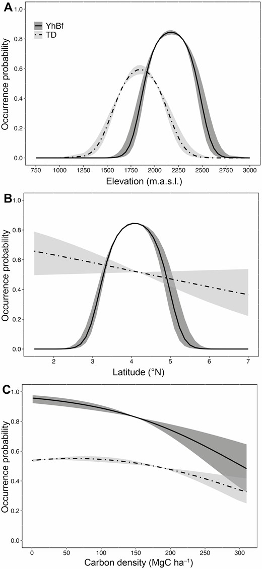
Variation in occurrence probability of Yellow-headed Brush-finch and Tolima Dove across the Colombian Andes as a function of regional and local predictors. Predictions from occupancy-detection models for the two species are presented as a function of (A) elevation, (B) latitude, and (C) vegetation density (aboveground carbon density). Shown are the estimated coefficients (solid and dashed-dotted lines) and the standard error of the predicted values (±SE).
Spatial Distribution, AOO and Habitat Loss
Field surveys confirmed the presence of both species in 3 new localities where their occurrence was previously unknown or unverified. These new records were mostly located in areas previously presumed to represent range discontinuities for each species (Figures 3 and 4).
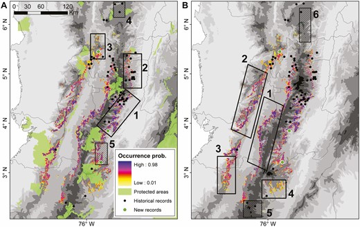
Identification of (A) priority conservation areas and (B) important areas for future research efforts for Yellow-headed Brush-finch across the Colombian Andes. The species’ area of occupancy (AOO) is represented as a spatial projection of its occurrence probability based on occupancy-detection models. New localities for the species reported in this study are represented by green dots. Left panel: clear and striped areas represent unprotected regions and locations in the vicinity of protected areas, respectively. Right panel: clear and striped areas represent regions of high occurrence probability and areas with recent records without suitable habitat, respectively.
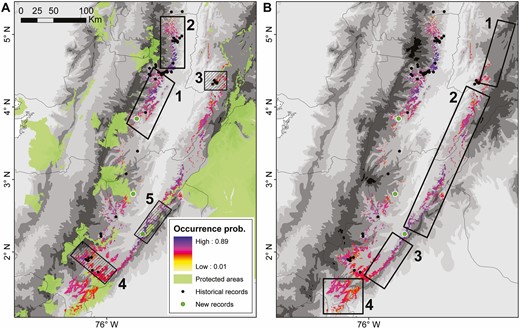
Identification of (A) priority conservation areas and (B) important areas for future research efforts for Tolima Dove across the Colombian Andes. The species’ AOO is represented as a spatial projection of its occurrence probability based on occupancy-detection models. New localities for the species reported in this study are represented by green dots. (Left panel) Clear and striped areas represent unprotected regions and locations in the vicinity of protected areas, respectively. (Right panel) Clear and striped areas represent regions of high occurrence probability and areas with recent records without suitable habitat, respectively.
Distribution models were defined as spatial projections of occurrence probability based on the predictors from the best model for Yellow-headed Brush-finch and model-averaged values from the best 2 models for Tolima Dove (Supplementary Material Figures S5 and S6). We estimated an AOO of 4,251 km2 for Yellow-headed Brush-finch and of 2,755 km2 for Tolima Dove. These estimates are above the IUCN thresholds used for threat categorization under criterion B2. We estimated that Yellow-headed Brush-finch and Tolima Dove had respectively lost ~44% and ~40% of their original habitat as of 2012, and that habitat loss rates during 2002–2012 were ~6–8% for both species. Our analyses suggest that only 17% and 10% of the remnant habitat of Yellow-headed Brush-finch and Tolima Dove is represented within protected areas, and that they overlap with 132 and 121 small private reserves, respectively.
Visual Inspection of Priority Areas
We identified 5 priority conservation areas within the AOO of Yellow-headed Brush-finch (Figure 3). Three areas with high occurrence probabilities coincided with unprotected population strongholds, 2 of them located on the Central Andes in the departments of Tolima and Caldas (areas 1 and 2 in Figure 3A), and a third in the Western Andes covering parts of Risaralda and Antioquia (area 3 in Figure 3A). The remaining 2 areas are in the vicinity of protected areas, one at the northern limit of the species distribution where it was recently recorded (area 4 in Figure 3A), and another in Tolima where we report a new locality (area 5 in Figure 3A). In addition, 6 important areas for future research were identified. Four of these areas with high occurrence probabilities are located in the Central (areas 1 and 4 in Figure 3B) and Western (areas 2 and 3 in Figure 3B) Andes. The other 2 areas are at the northern and southern limits of the species’ distribution where presence records exist.
Five priority conservation areas within the AOO of Tolima Dove were identified, the first two coinciding with unprotected areas of high occurrence probabilities and overlapping with important areas for Yellow-headed Brush-finch in Tolima and Caldas (areas 1 and 2 in Figure 4A). Three important areas neighboring protected areas were located, 1 near the southern range limit (area 4 in Figure 4A), and 2 along the Eastern Andes where the species was recently discovered (areas 3 and 5 in Figure 4A). We also identified 4 key research areas, 3 of them along the Eastern Andes (areas 1–3 in Figure 4B), and 1 near the Colombian Massif where information on the species presence is non-existent (area 4 in Figure 4B).
DISCUSSION
We used a protocol based on the sequential application of ENMs and occupancy-detection models to provide the most complete and up-to-date hypotheses of the distribution of the Yellow-headed Brush-finch and Tolima Dove, 2 species whose presence outside the Central Andes of Colombia was confirmed only recently (Calderón-Franco et al. 2012, López-Ordóñez et al. 2013, González-Prieto et al. 2014). Overall, our analyses point to more extended and more continuous distributional ranges for both species, but also provide an early warning (hopefully) of the lack of representation of these 2 birds in the Colombian national protected areas system (SINAP). Our approach provides an example of how using different methodologies can help maximize limited information to generate highly detailed, accurate distribution models to identify conservation priorities for data-poor species. Below we discuss in detail the scope and limitations of this approach, and the main implications for conservation and future research.
A Simple, Cost-Efficient Protocol for Modeling Data-Poor Species
Our 2 study species provide a good example of a common trade-off that conservation biologists face when assessing the extinction risk of data-poor taxa: balancing the impossibility of collecting data representative of a species entire geographical distribution due to logistical and funding limitations, against using often scarce and spatially biased geographical information to run species distribution models that in turn may lead to erroneous assessments. The approach presented here may offer a simple alternative that can be applied to a number of species of conservation concern. A first step consists of using publicly available data to study the climatic correlates of a species’ distribution and to identify habitable areas in geographic and climatic space. With this information, it is then possible to design a time- and cost-efficient sampling scheme for collecting data at a limited but environmentally representative number of localities, for subsequently generating accurate distribution models that account for imperfect detection. These models can later be used to identify areas with high occurrence probability, which might be helpful in guiding future conservation actions and for filling gaps in scientific knowledge.
We think it is important to emphasize the relevance of carefully evaluating and correcting spatial biases in occurrence data, particularly when working with priority species. Considering that numerous rare and threatened species are data deficient (see, e.g., Renjifo et al. 2014, 2016), modelers often do not assess the quality of input data to avoid reducing an already limited sample size. However, as data for range-restricted taxa tend to be spatially and environmentally autocorrelated (Franklin and Miller 2010, Peterson et al. 2011), modeling with autocorrelated data can cause overfitting, and ultimately, underestimated distributions (Veloz 2009, Fourcade et al. 2014, Cardador et al. 2017). Our preliminary analyses, for example, revealed spatial clustering in Yellow-headed Brush-finch data and high environmental-spatial autocorrelation for the Tolima Dove, highlighting the importance of using spatial filtering before fitting ENMs. Regardless of the existence of preventive (e.g., assessing for autocorrelation; Botero-Delgadillo et al. 2015a) and corrective techniques to reduce overfitting (e.g., spatial rarefaction; Boria et al. 2014) and overprediction (e.g., model clipping; Kremen et al. 2008), application of these methods is still not common practice. We adhere to the call from other authors for incorporating graduated spatial rarefaction as a standard practice when modeling climatic niches (Veloz 2009, Boria et al. 2014).
Our results also highlight the relevance of including factors potentially affecting the detection process into modeling exercises, so as to generate credible distribution hypotheses for rare species. This is well illustrated by the Tolima Dove, a species whose ecology is still poorly understood partly due to its relatively secretive habits (Carvajal-Rueda et al. 2014, Baptista et al. 2020). Our data indicated that the species’ detection probability was particularly low when using passive counts; hence, the use of playback counts and the need to incorporate the effect of survey methodology on detectability in the process of modeling occupancy. Accounting for imperfect detection is seldom put into practice, and most distribution models for priority species are frequently built based on the assumption of “perfect detection” (i.e. every absence in the data is taken as a true absence). The problem with this assumption is that it rarely holds, and its violation can increase the rate of false negatives in a dataset and result in erroneous predictions (MacKenzie et al. 2003, Kéry and Schmidt 2008, Lahoz-Monfort et al. 2014).
To conclude this section, we briefly discuss some of the limitations of our protocol, a necessary step before interpreting the resulting distribution models and their implications for our study species. First, some of the historical localities used for ENMs require reconfirmation of the species’ presence; hence, there is high uncertainty regarding the models’ predicted suitability, either high or low, for these areas. For instance, the presence of Yellow-headed Brush-finch nearby the Meremberg Natural Reserve (area 5 in Figure 3B) was reported 41 years ago (Ridgely and Gaulin 1980) but, to the best of our knowledge, there are no subsequent records. Few records used in this study are believed to come from areas where either Yellow-headed Brush-finch or Tolima Dove may no longer occur, and thus bias in the niche modeling process is likely low, but still these areas deserve careful attention (see below). Second, even though our field surveys were representative of the species’ climatic niche variation, we failed to include several areas along the Western and Eastern Andes, where the 2 species have not been searched for. This may have affected our ability to estimate the influence of Andean range on each species’ occurrence probability (although see results for Tolima Dove in Table 4).
Conservation Priorities and Important Areas
Our results suggest that the 2 study species exhibit a relatively restricted distribution along a narrow Andean belt at mid-elevations (~1,300–2,600 m.a.s.l.), mostly in the Central Andes, with isolated populations in the Eastern and Western Andes of Colombia. The Central Andes may have lost up to 80% of their original vegetation cover (Etter et al. 2008, 2015), particularly at mid-elevations where coffee plantations dominate the landscape (Guhl 2008, Corrales Roa 2012). This has likely impacted a number of range-restricted and endemic birds mostly occurring along the Central (as well as the Eastern) Andes and the inter-Andean slopes, including the Yellow-headed Brush-finch and Tolima Dove (Corrales Roa 2012, Renjifo et al. 2014). Across the range of these 2 species, human settlements keep growing and agricultural expansion is still a major threat, drastically reducing the areas where they can survive. Previous evaluations (Renjifo et al. 2014) and our results strongly indicate that habitat loss still persists, which makes the situation more critical, as these two birds are considered “gap species” given that only 10–17% of their remnant habitat is represented within protected areas.
Although both species appear to tolerate human-altered landscapes, it is still uncertain whether survival and reproductive success are comparable between transformed and primary habitats. The Yellow-headed Brush-finch is often associated with regenerating vegetation and early successional stages (Botero-Delgadillo et al. 2022), but its breeding habitat is poorly known (Molina-Martínez 2014). Similarly, Tolima Dove has been observed in coffee plantations and cattle pastures (Carvajal-Rueda et al. 2014), but it is not known whether these habitats could act as ecological traps. Our study did not provide further insight into habitat selection patterns for Yellow-headed Brush-finch and Tolima Dove, as none of the top-ranked models suggested habitat as an important predictor of their occurrence. It is possible that habitat characteristics and vegetation cover may affect each species at a larger scale than the one we used for determining habitat type (each transect covered ~0.5 ha), but this needs confirmation. In any case, our models indicated that their occurrence probabilities are higher in areas with relatively low to moderate vegetation cover (i.e. areas of mixed vegetation). Based on published information (Birdlife International 2021a, 2021b) and the results presented here, we hypothesize that both species may thrive in agricultural landscapes, provided they contain remnants of natural vegetation. This means that their populations are likely to do well in response to management actions that are potentially feasible (e.g., creating more riparian buffers, hedgerows, etc.).
Spatial distribution models and occurrence probabilities suggested 5 regions of high importance for each species, two of which comprise an extensive area of co-occurrence in northwestern Tolima (areas 1 and 2 in Figures 3A and 4A), and largely overlap with the Colombian inter-Andean slopes endemic bird area (EBA 040; BirdLife International 2021c). This region may represent a stronghold for both Yellow-headed Brush-finch and Tolima Dove populations, as density estimates for both species are higher there and the region also holds the majority of historical records (Escudero-Páez et al. 2018a, 2018b). Unfortunately, this area is largely underrepresented in protected areas and it is still being severely affected by forest clearance. Increasing the representation of protected areas within this region (and also in area 3 for Yellow-headed Brush-finch; Figure 3A) is thus a priority not only for our study species, but for other co-occurring endemic species such as the Tolima Blossomcrown (Anthocephala berlepschi; VU), Yellow-headed Manakin (Chloropipo flavicapilla; VU), and Crested Ant-tanager (Habia cristata; LC).
Given that declaring new protected areas or extending already existing ones is not feasible in all priority regions, alternative conservation actions should focus on the design of best management practices in agricultural systems like coffee plantations, simultaneously protecting the species and strengthening agricultural production (e.g., Bennet et al. 2018). Other complementary actions include avoiding habitat loss in rural landscapes by maintaining remnants of natural vegetation along water courses, and by increasing available habitat for both species via conservation agreements with landowners (Escudero-Páez et al. 2018a, 2018b). These actions may also be helpful in priority regions where managers of public and/or private protected areas could work alongside local landowners to design an integrated management strategy promoting the establishment of a connected mosaic landscape (e.g., areas 4 and 5 in Figure 3A, and 3–5 in Figure 3B). To this end, initiatives promoting the regeneration of natural vegetation and the establishment of natural corridors will be essential. These may prove valuable not only for resident species, but also for priority Nearctic–Neotropical migratory birds that winter in mid-elevation Andean ecosystems, for example, the Canada Warbler (Cardellina canadensis), Cerulean Warbler (Setophaga cerulea), Acadian Flycatcher (Empidonax virescens), and Olive-sided Flycatcher (Contopus cooperi) (González et al. 2020, Céspedes et al. 2021).
Knowledge Gaps and Areas for Future Research
Both study species were recently downlisted from Endangered (EN) to Near-Threatened (NT) in the IUCN Red List given that their current distributions are now suspected to be larger than previously thought (BirdLife International 2021a, 2021b). Our AOO estimations for both species (Yellow-headed Brush-finch: 4,251 km2, Tolima Dove: 2,755 km2) also support larger distributions and are less conservative than the estimated values from the last detailed evaluation of their risk of extinction (Renjifo et al. 2014; Yellow-headed Brush-finch: 647 km2, Tolima Dove: 1,160 km2). One reason for these differences is that the species’ known distribution ranges have increased as new records in previously unknown localities have accumulated, including the new localities reported in this study. In addition, our analyses considered mosaic areas (i.e. agricultural landscapes interspersed with native vegetation) as feasible habitat, meaning that large parts of the AOOs reported here include vegetation types that are not used by the species, such as grassland and annual crops. As the resolution of available landcover data does not allow for a more precise estimate of the amount of suitable habitat within mosaic landscapes, we propose that a more conservative and perhaps realistic estimate of their AOOs would be closer to 2,760–3,740 km2 for Yellow-headed Brush-finch and 1,620–2,370 km2 for Tolima Dove (assuming that 25–75% of the extension of mosaic landscapes comprises suitable areas for the species).
Even though both species mainly co-occur between 1,600 and 2,000 m.a.s.l., ENMs suggest they may favor different climatic conditions throughout their ranges. The Yellow-headed Brush-finch is associated with premontane and montane areas with low seasonality in temperature and precipitation, whereas the Tolima Dove appears to mainly occur in premontane areas with mild temperatures and a more marked variation in precipitation. These conditions extend along the length of the Andean slopes and may allow populations of both species to be more continuously distributed than previously thought, as our models and recent records imply. We identified four areas for each species where future research efforts could confirm their presence in ecologically suitable areas that connect apparently disjunct populations (areas 1–4 in Figures 3B and 4B). Nearly a decade ago, both species were presumed to be disjunctively distributed along the Central Andes (see BirdLife International 2021a, 2021b), but our results suggest otherwise. Therefore, expecting a more continuous distribution along the Western (for the finch) and Eastern (for the dove) Andes is reasonable, but this needs confirmation.
We also identified 2 areas on the range margins of the Yellow-headed Brush-finch where field surveys are needed and where environmental suitability is low (areas 5 and 6 in Figure 3B). At the southern margin, the species was recorded nearby the private Meremberg Natural Reserve during the 1980s (Ridgely and Gaulin 1980), but its presence in this protected area and the neighboring Puracé National Park is yet to be confirmed. At the northern margin, habitat loss and transformation are high, but there are recent records uploaded to eBird confirming the presence of the species in thickets and bushy borders along main roads. Whether or not there is a healthy population there is unknown.
Aside from the distribution gaps needing urgent study, there are other relevant aspects of the species’ ecology that are poorly known. First, it is urgent to establish whether abundance and density vary with the percentage of natural vegetation in rural landscapes (Escudero-Paéz et al. 2018a, 2018b). Second, it is necessary to collect more data on the species’ reproductive biology, to facilitate comparisons of productivity parameters between habitat types (Botero-Delgadillo et al. 2021). Third, it would be worthwhile to determine how interconnected populations are between and within the Andean ranges, and whether landscape connectivity is a limiting factor for dispersal among populations. And fourth, it would be useful to collect more presence–absence data, to enable describing temporal changes in occupancy (see Briscoe et al. 2021) and to obtain predictions of the species’ range dynamics as a function of habitat transformation.
Prospects and Concluding Remarks
Several studies have aimed to assess the risk of extinction of target species, mostly relying on the use of ENMs that are processed post hoc, either by combining them with land cover layers to model distributions (e.g., Botero-Delgadillo et al. 2012a, 2012b) or to estimate areas of occupancy (AOO; e.g., Renjifo et al. 2014, 2016). Although valuable and necessary, this approach frequently leads to misinterpretations and biased conclusions that may obstruct efforts to identify important areas for conservation. First, spatial projections of ENMs are sometimes interpreted as predictions of a species’ probability of occurrence, when in reality they represent environmental suitability for its presence. As a result, it is not really possible to spatially identify areas of conservation importance or population strongholds, which is only possible with “true” estimations of species’ occupancy or abundance/density. Second, post-hoc processing is usually based on “expert criteria” to decide which areas should be removed from the spatial projection of ENMs (e.g., Renjifo et al. 2014), making the modeling process prone to subjectivity. The protocol used here (i.e. sequentially using ENMs with occupancy models) may prove valuable as it provides a straightforward approach that maximizes available information, while allowing for the “true” estimation of occurrence probabilities. This approach provides a simple and efficient solution for producing high-quality information with limited resources, as this is certainly the case for several projects focused on tropical priority species.
ACKNOWLEDGMENTS
We want to thank all the individuals who assisted surveys at localities throughout Colombia. Special thanks go to the following organizations for their logistical support: Corporación para el fomento del Aviturismo en Colombia CORAVES (Neira, Caldas), Organización Ambiental Vida Silvestre (Apía, Risaralda) and the Corporación Autónoma Regional del Alto Magdalena CAM.
Funding statement: This work was funded by the American Bird Conservancy (agreement #1771A) as part of a project on identifying key areas for the conservation of the Yellow-headed Brush-finch and the Tolima Dove.
Ethics statement: No birds were captured or manipulated during this study. Fieldwork protocols were approved under Resolution No. 179-2015 from Parques Nacionales Naturales de Colombia and Resolution 0597-2014 and 0189-2016 from Autoridad Nacional de Licencias Ambientales (ANLA) issued to SELVA.
Author contributions: E.B.-D., S.E.-P. and N.B. conceived the idea and supervised the research. J.S.-M. and P.C. collected the data and lead field expeditions. E.B.-D. analyzed the data and wrote the manuscript with input from N.B.
Data availability: Analyses reported in this article can be reproduced using the data provided by Botero-Delgadillo et al. (2021).
