


Abstract
Forecasting changes in size and distributions of populations is an essential component of conservation assessments. Such forecasts are only useful for species conservation and management when they are based on robust estimators of fecundity, survival, and density dependence. While apparent survival estimation is the main focus of mark–recapture modeling, fecundity and density dependence are rarely the subject of these models. Here, we present a Bayesian hierarchical framework that can estimate fecundity and density dependence along with age-based survival using only robust-design capture–recapture data. We refer to this framework as RD-pop. We used simulated capture histories to demonstrate that RD-pop can estimate vital rates and their density dependence with little bias. We applied RD-pop to capture history data from Brown Creeper (Certhia americana) and showed that estimates of fecundity are consistent with the breeding biology of this species. Finally, we illustrate that density dependence, even when estimated with uncertainty in the RD-pop framework, regularizes population dynamics and reduces the frequent population extinctions and explosions observed under density-independent models. RD-pop is a useful addition to the current mark–recapture modeling toolbox especially when the goal is to build population models that can make medium- and long-term projections. It can be applied to any population for which long-term robust-design mark–recapture data are available, and with slight modifications (incorporation of weather and climate effects on vital rates) has the potential to facilitate demographic projections under climate change.
Resumen
Pronosticar cambios en el tamaño y la distribución de las poblaciones es un componente esencial de las evaluaciones de conservación. Estos pronósticos solo son útiles para la conservación y el manejo de especies cuando se basan en estimadores robustos de fecundidad, supervivencia y dependencia de la densidad. Si bien la estimación de la supervivencia aparente es el enfoque principal del modelo de marca-recaptura, la fecundidad y la dependencia de la densidad rara vez son considerados por estos modelos. Aquí, presentamos un marco de trabajo jerárquico bayesiano que puede estimar la fecundidad y la dependencia de la densidad junto con la supervivencia basada en la edad, utilizando solo datos de captura-recaptura provenientes de un diseño robusto. Llamamos a este marco de trabajo como RD-pop. Usamos historias de captura simuladas para demostrar que RD-pop puede estimar las tasas vitales y su dependencia de la densidad con poco sesgo. Aplicamos RD-pop para capturar datos históricos de Certhia americana y mostramos que las estimaciones de fecundidad son consistentes con la biología reproductiva de esta especie. Finalmente, ilustramos que la dependencia de la densidad, incluso cuando se estima con incertidumbre en el marco de RD-pop, regulariza la dinámica poblacional y reduce las extinciones y explosiones poblacionales frecuentes observadas bajo modelos independientes de la densidad. RD-pop es una herramienta adición útil para los modelos de marca-recaptura actuales, especialmente cuando el objetivo es construir modelos poblacionales que puedan hacer proyecciones a mediano y largo plazo. Puede aplicarse a cualquier población para la que se disponga de datos de largo plazo de marca-recaptura de diseño robusto, y con ligeras modificaciones (incorporación de los efectos meteorológicos y climáticos en las tasas vitales) tiene el potencial de facilitar las proyecciones demográficas bajo cambio climático.
Lay Summary
• Population dynamics models are used to predict how populations of species will change in the future. These models require estimates of the population’s survival rates, fecundity rates, and how these rates change with population density.
• One of the most common and useful types of data is obtained by marking (banding, tagging) individuals and recapturing (or resighting) them. These mark–recapture data are rarely used to estimate fecundity and density dependence, and consequently, to parameterize population models.
• We present a framework that employs mark–recapture data to build population models to inform conservation decisions on bird species. We show that this framework can estimate fecundity and density dependence parameters with little bias. We demonstrate this by using simulated population data as well as empirical mark–recapture data of Brown Creeper (Certhia americana).
• We show that when parameters estimated with this framework are used to project population abundances, the distributions of conservation-relevant metrics (such as minimum abundance of a population) are close to the true distributions obtained by simulations.
• This framework provides a useful alternative to building population models for making conservation decisions in countries that lack long-term count data such as Breeding Bird Survey in North America.
INTRODUCTION
Forecasting changes in size and distributions of populations is at the forefront of ecological sciences in the 21st century. Population viability analysis (PVA) is one of the earliest methodological frameworks to adopt forecasting as its core mechanic in order to inform decisions related to single-species conservation (Boyce 1992, Akçakaya and Sjögren-Gulve 2000, Beissinger and McCullough 2002). A successful PVA requires “rigorously estimated demographic parameters using the best available data” (Chaudhary and Oli 2020), including, at a minimum, fecundity (along with age at first breeding), age-structured survival, and temporal variability. Additionally, density dependence is a necessary component of population forecasts, because without a density-dependent check, populations can be predicted to grow exponentially to levels that are not biologically feasible. Capture–recapture data, in this context, have not been fully utilized to parameterize population models used in PVAs, namely: (1) fecundity is rarely estimated from capture–recapture data (e.g., Nichols and Pollock 1990); (2) density dependence estimation has been the subject of relatively few studies and usually with a focus on single-population dynamics, making it unfeasible to generalize demographic parameters to meta-population PVAs (e.g., Tenan et al. 2019); and (3) the majority of mark–recapture models estimate only a subset of demographic parameters that are required by PVAs, and in the rare instances in which they estimate all these parameters, the parameters are estimated independently from one another, not accounting for statistical and ecological relationships among them (e.g., Ryu et al. 2016).
Fecundity is a measure of breeding performance of a population and, in the context of a PVA, can be defined as the per-capita number of offspring that survives to the next time step without any immigration component (Akçakaya et al. 1999). When no explicit data on fecundity are available, models such as Jolly-Seber (JS) models and even some integrated population models (IPM; e.g., Ahrestani et al. 2017) estimate recruitment rate as the total number of individuals added to a population in a given time period, which includes both immigrants and new-born individuals. Recruitment rate, in this regard, is different from fecundity and is not useful for making age-structured population projections, because density dependence and stochasticity in fecundity cannot be explicitly accounted for in this parameter alone. A PVA that employs an age-structured matrix model requires both the number of juveniles born per individual and the juvenile survival to be explicitly estimated (Ryu et al. 2016).
Density dependence (DD) is the phenomenon of population vital rates being dependent on population size. Along with exogenous factors, it is one of the main natural processes that regulates population dynamics. It is widespread in natural populations and can be detected from time-series data with mixed success (Brook and Bradshaw 2006). While there are examples of estimating the strength of density dependence from mark–recapture data (Gullett et al. 2014, López-Roig and Serra-Cobo 2014, Troyer et al. 2014, Nater et al. 2018, Tenan et al. 2019), it is rare that these estimates can be used for population projections. The main issue is that most studies use population abundance as a direct covariate when modeling density dependence. This approach can become problematic with more than one population, especially when each population has different habitat characteristics and therefore can support different number of individuals. If the goal is to estimate a species-specific average density dependence strength that is applicable across all populations of the species, abundance of each population in each time step should be standardized with a proxy for how many individuals each population can support (e.g., carrying capacity; Ryu et al. 2016).
Capture–recapture methods are highly diverse, but each independent method usually only estimates a small number of parameters, focusing on distinct processes such as survival, recruitment or immigration, and emigration (Williams et al. 2002, Cooch and White 2016). Integrated population models are an exception as they can estimate a full array of demographic parameters, enough to make population forecasts, but they require count data in addition to mark–recapture data (Schaub and Abadi 2011). Ryu et al. (2016) is the only framework we are aware of that can estimate all demographic parameters necessary to build a population model with only mark–recapture data. Ryu et al. (2016)’s framework, however, builds independent models that inform one another in a sequence. For example, they first built a Cormack-Jolly-Seber (CJS) model to estimate abundances and densities of populations and then used these density estimates in another model as a variable to estimate density dependence strength on survival. There are two issues with this approach:
(1) When using the output of one model as an input in another independent model, the input is usually a point estimate (e.g., the mean) that ignores the uncertainty associated with the estimate. So, the uncertainty in parameter estimates does not propagate through connected models, and the end result might appear more certain than it actually is, which will lead to narrower confidence intervals.
(2) In density-dependent population regulation, all vital rates are connected. Their independent estimation may not provide results that are consistent with density-dependent dynamics; for example, models might estimate positive or negative growth at carrying capacity instead of no growth.
Here, we present a Bayesian hierarchical framework that can estimate age-dependent and density-dependent survival and fecundity, and temporal variance in vital rates, using only robust design mark–recapture data. We base this framework on Ryu et al. (2016) but all models associated with the framework are fit simultaneusly with proper error propagation. We also explicitly account for the expected relationships among vital rates under density dependence, and as a result, estimate ecologically meaningful juvenile survival rates. Because this framework employs a robust design and population-level covariates in its functions of vital rates and capture probabilities across multiple populations, and because of its focus on building population models, we call it hereafter “RD-pop” throughout this manuscript. In addition to demonstrating RD-pop, we present here a simulation system that extends the framework presented in Abadi et al. (2010) by including density dependence and environmental stochasticity. We use this simulation framework to detect parameter estimation biases in RD-pop. Finally, we demonstrate the usefulness of RD-pop with a particular focus on the necessity of density dependence when forecasting with age-structured matrix population models and calculating conservation-relevant metrics such as expected minimum abundance (McCarthy and Thompson 2001), which is commonly used as a risk measure in PVA models.
METHODS
RD-Pop
RD-pop requires, at minimum, two types of data: robust-design capture histories and annual number of captured adults and juveniles, which can be obtained from said capture histories.
(1) Capture history. RD-pop employs robust-design capture histories (Kendall et al. 1995) where there are multiple secondary capture occasions in a primary capture period. For example, in the test dataset we used (described later), every year in the 17-year period from 1992 to 2008 is a primary capture period, and each month in the breeding season from May to August constitute the secondary occasions. Capture of a marked individual in a secondary occasion is assigned 1, and failure of capture is assigned 0. Robust design combines open and closed population mark–recapture models. Within a primary period (here, the breeding season) populations are assumed to be closed (no mortality and no emigrations; see the Discussion for additional justification of population closure assumption of adults and juveniles) and capture probability is estimated with captures between secondary occasions (months). This capture probability can then be used to estimate population size. Between primary periods populations are assumed to be open (individuals can die or leave the population). Survival is estimated with capture information obtained from primary periods (for example, if an individual is captured at least once in a primary period we know it survived from the previous primary period). Additionally, we assume no temporary emigration in the robust design of RD-pop (γ’ = 1 and γ” = 0; see Cooch and White (2016)).
(2) Number of captured adults and juveniles. We count the number of adults and juveniles captured or recaptured at least once per year in each population. Using these counts and estimated capture probabilities from the robust design, we estimate a population-level density index, as well as fecundity (as number of juveniles per adult). Here, we group mist-netting stations into separate populations, in accordance with the data set used for modeling Brown Creeper population dynamics (see Parameter Estimation with RD-pop). While we only considered a population structure with two age classes in this study, the framework we present can be applied to other types of age and stage structures in populations.
A survival rate estimated with mark–recapture models is called apparent survival, because it is the joint probability of surviving and staying in the population. Apparent survival rates tend to be lower than true survival rates and may lead to biased projections if used in population models. Here, we used an additional data type to explicitly model resident and transient individuals to correct this potential bias. This is not a mandatory part of RD-pop and can be omitted if there are not many suspected transient individuals of a modeled species. The residency model uses pre-determined residents as the third dataset of RD-pop presented here:
(3) Pre-determined residents. This is a binary variable. A captured individual is categorized as a pre-determined resident if it was recaptured at least once >10 days following its first capture in its initial year of capture (Royle and Dorazio 2009, Ahrestani et al. 2017). The rest of the individuals are categorized as potential transients. Transient adult individuals are assumed to be passing through the population (they will not stay and breed); transient juvenile individuals are assumed to leave the population after fledging. Residents categorized this way are named pre-determined, because their categorization happens before running any model (Saracco et al. 2010). Pre-determined residents are assigned 1 and potential transients 0 in this data set. The 10-day threshold can be changed with ecological justifications (for example, Saracco et al. (2010) used 6 days) but its effect on the results we present is minimal.
These 3 data sets, derived from the same robust-design capture histories, are used to build 5 connected models and estimate their associated parameters: Survival, Capture, Density, Residency, and Fecundity (Figure 1).
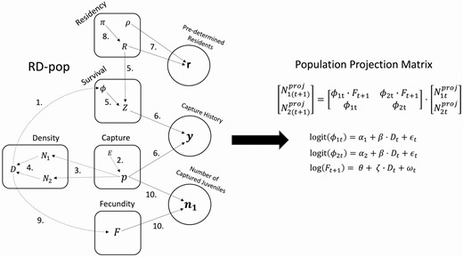
(left) RD-pop: Graphical representation showing how model parameters relate to each other, to variables, and to data. Each circle is a separate data entry to the modeling system. Rounded rectangles represent interconnected models (Capture, Survival, Residency, Fecundity) or a set of equations for derived variables (Density). Arrows indicate stochastic (solid arrows) or deterministic (dashed arrows) relationship among parameters, data and variables. Parameters are shown without subscripts to simplify the illustration. The numbers on arrows refer to the Equation numbers in the main text. (right) Population Projection Matrix: Parameters estimated by RD-pop are used to build an age-structured population model for making population projections. See the main text for parameter descriptions. Note that we omitted the population subscript (k) from the parameters in the matrix to signify that this is the matrix of a single population.
Survival
Survival is modeled as a function of age class (juvenile or adult), and a population density index:
Where, x = 1,2,….,X and x = 1,2 with two age classes; k = 1,2,3,….,K; t = 1,2,3,….,T; is the survival probability of an age class x individual at population k and year t; α x is the survival probability of an age class x individual on logit scale at mean population size (juveniles are coded as 1 and adults as 2) in an average year; β is the change in survival on logit scale with one unit change in population density index; Dk,t is the population density index at population k and year t, this index is 0 at mean population size (see Density section); ∊ t is the temporal random effect at time t, and σ 2s is the temporal process variance of survival at logit scale, which assumes full correlation between populations in their temporal variability (all populations have the same temporal effect each year).
Capture
Capture probability is modeled as a function of effort and age class:
where, h = 1,2,3,….,H; px,k,t,h is capture probability of an age class x individual at population k, year t, and month h; γx is the monthly capture probability on logit scale of an age class x individual at mean capture effort; δ is the change in monthly capture probability on logit scale with one unit change in capture effort; and E is the capture effort.
Density
The monthly capture probabilities obtained from the capture model are used to calculate the yearly capture probabilities, and these in turn are used to estimate the expected size of each population in each year. Yearly capture probability for each adult and juvenile in a given year and population is calculated as follows:
where, p*x,h,t is the probability that an age class x individual will be captured at least once in 4 months of the breeding period at year t and population k.
Using the heuristic estimator for population size (first term on the right-hand side of Eq. 3b) with a correction for years with 0 captures (Dail and Madsen 2011; second term on the right-hand side of Eq. 3b), the numbers of adults and juveniles can be derived as:
where, nx,k,t is the number of captured age class x individuals in population k and year t, and Nx,k,t is the expected number of age class x individuals of the same population and year combination.
Expected total population size of population k at year t, Mk,t, is estimated by adding up N1,k,t and N2,k,t. Density index of population k at year t, then, is estimated as:
where, T is the number of years with capture effort in population k. Because relative density is calculated by dividing each year’s population size (numerator in Eq. 4) by the average size of that population across years (denominator in Eq. 4), average relative density of a given population is always 1. When modeling survival and fecundity, we used this information to centralize the relative density estimate around its mean by subtracting 1 and refer to this metric as population density index (D). The centralized nature of this metric increases the effective number of samples in the posterior chains of the density dependence strength parameters estimated by survival and fecundity models (β and ζ, respectively).
Eq. (3b) is not defined for when capture probability is 0. Because capture probability is modeled on a logit scale it will tend asymptotically towards 0. This asymptotic behavior can lead to small capture probabilities and therefore large abundances in years with no capture effort. So, in years with no capture effort, instead of using Eq. (3b), we assumed that the population was at its average abundance, which effectively is equal to a density index value of 0. We set the limits of a time series of a population with the first and last years of capture effort in that population and assumed average abundance only if there was no capture effort in a year within the limits of a time series. There were only 3 such populations out of 43 with a total of 10 years of no capture effort.
State and Observation Processes
Survival and capture probabilities are functions of population-level covariates (population density index and effort, respectively). However, capture history data are at the individual level, so there needs to be a link between population-level parameters and individual-level data. We made this link by using the matrix Si,t to indicate the age class of the ith individual in year t, and the vector gi to indicate the population that the ith individual is in.
The state of the ith individual (alive and in the population or not) in year t + 1, Zi,(t+1), depends on whether it was alive at time t, whether it survived the period from t to t + 1, and whether it is a resident. This latent state is a Bernoulli random variable:
where, ϕ(Si,t),(gi),t is the survival probability at the age class and population of the ith individual from year t to t + 1, and Ri is the true residency status of the ith individual (1 if it is a resident, 0 if it is a transient).
Every element of the capture history, yi,t,h (1 if an individual is captured, 0 if it is not), is a Bernoulli random variable with a monthly capture probability, p(Si,t),(gt),t,h, conditional on the individual is alive, and in the population, Zi,t.
Residency
We employed a simplified version of the models described in Hines et al. (2003) and Nott and DeSante (2002) when modeling residents. This approach accounts for transients that will leave the population after their first capture but does not model movement between populations. We assumed that there are two parameters, ρ1 for juveniles and ρ2 for adults, that governs the probability that we can correctly categorize a true resident as a pre-determined resident. The residency data (1 for pre-determined residents, 0 for potential transients), ri, is a Bernoulli random variable and is conditional on the ith individual being a true resident (Ri):
where, fi is the first capture year of the ith individual, and Si,fi corresponds to the age class of the ith individual in its first capture year. We also assumed that there is a parameter for each age class, π 1 and π 2, that governs the probability that a juvenile or an adult in the population is a true resident, respectively. Ri is a Bernoulli random variable with probability πSi,fi:
In this formulation, 2 separate parameters are necessary because the categorization of individuals as pre-determined residents or as potential residents is the product of 2 processes, one for the true residency status of the individual (π) and one for our ability to categorize one as true resident if it really is a resident (ρ).
This model effectively filters out some of the capture histories that only have the first capture followed by no captures for the remainder of study period (a single 1 and trailing 0s in their capture history). If true residency of an individual (R) is estimated to be 0 (a transient), then its state (Z), will also be automatically 0 (see Eq. 5) and it will not lower the survival estimate. π and ρ are nuisance parameters and are not used in projections explained below.
Fecundity
We followed Ryu et al. (2016)’s fecundity definition: the annual ratio of fledged juveniles to adults for each defined population. Because the age of first breeding in this model is 1, and fecundity does not change with age, juvenile to adult ratio is an estimate of fecundity. Thus, we use the term fecundity for this variable in our model, although this would not be strictly correct for other models. Fecundity in population k and year t + 1, Fk,(t+1) was estimated as a function of density index at year t, Dk,t, with a log link:
where θ is the average fecundity in log scale at mean population size in an average year; ζ is the change in fecundity in log scale with one unit change in population density index; ωk,t is the spatio-temporal random effect at population k and time t; and σ2f is the spatio-temporal variance of fecundity, which assumes 0 correlation between populations in their temporal response (each population in each year can have a different and independent random effects). See Supplementary Material S2 for a detailed discussion of why the structure of random effects of survival and fecundity are different.
This function is then linked to the observed number of juveniles (n1,k,t) as a zero-inflated Poisson model:
where Fk,t is fecundity; N2,k,t is the expected number of adults (Eq. 3b); p*1,k,t is the annual capture probability of juveniles (Eq. 3a) at population k and year t; ψ is the probability that the number of captured juveniles in a given year and population is not 0; and wk,t is the indicator as a Bernoulli random variable stating whether number of captured juveniles in population k and year t is higher than 0. In this fecundity model, we only included years and populations that had at least 1 adult capture. We used a zero-inflation model because its fecundity estimates were biologically more realistic and had Bayesian p-values closer to 0.5 compared to a regular Poisson model.
We also built a version of this framework without density dependence, consequently modeling only the average survival and fecundity. We contrasted population projections from this version with those obtained under models with density effects to demonstrate the regularizing effect of density dependence.
Connection to Age-Structured Matrix Models
The primary goal of RD-pop is to provide parameter estimates for age- or stage-structured population models (Figure 1). Almost all such models used for conservation purposes are discrete-time models, such as Leslie/Lefkovitch-type matrix models (Caswell 2001). Thus, they are essentially Markov models where the future state of the population depends only on its current state. When density dependence is incorporated into these models, density at time t affects the rates of transition (survival rates and fecundities) from time t to t + 1 (Caswell 2001). To provide parameters for these models, estimation methods must also relate density at time t to the transition rates (the matrix elements) that determine the transition from t to t + 1. This means the matrix assigned to time t + 1, which is the matrix that determines the state of the system in time t + 1, must be determined by the state of the system (including density) in time t. Thus, both survival from time t to t + 1 and fecundity at t + 1 is determined by density at time t.
RD-pop provides parameters for an age-structured matrix model based on an assumption of postbreeding census (Ryu et al. 2016). In these models, the rates of transition to juvenile stage are products of survival (of individuals from previous census to the current breeding season) and fecundity (Caswell 2001; Figure 1). When such models include density dependence, the assumption is that the intra-specific competition that occurs in the period from year t to t + 1 affects both the survival from last census to the current breeding season, and the reproductive capacity of the individuals, which is often determined by individual physiological condition at the start of the current breeding season. Additionally, the intra-specific competition is assumed to be a function of the total adult and juvenile population of the previous time step. This is a realistic assumption, because an average juvenile of last year will become an adult in the current breeding season and is likely to consume similar amounts of resources over this process with an individual that was an adult in the previous census.
We used the relationship among vital rates in an age-structured model with two age classes under density dependence to our advantage to estimate a juvenile survival rate with less uncertainty. We used information from adult survival and fecundity estimates, and the fact that they are density-dependent, to estimate juvenile survival:
where SJ and SA are survival rates of juveniles and adults at mean population size (inverse logit of α1 and α2, respectively) and F is the fecundity at mean population size (exponent of θ). This equation states that population growth rate (λ) is equal to 1 when population abundance is at it’s carrying capacity. We assumed that long-term average abundance of populations is an approximation of carrying capacity and used this equation to estimate juvenile survival as:
Parameter Estimation With RD-Pop
Mapping Avian Productivity and Survival (MAPS) is a collaborative mark–recapture program initiated and organized by the Institute for Bird Populations (IBP) since 1989 across 1,200 banding stations in US and Canada (Desante and Kaschube 2009). We applied RD-pop to Brown Creeper (Certhia americana) data obtained from the MAPS program. Brown Creeper is a widespread North American songbird species. It is a resident in the western U.S and along the coastline to Alaska, in north-eastern U.S, and southern Canada. It is a forest-dwelling bird and has a stable population trend (Birdlife International 2021).
We treated each MAPS location (a cluster of mist-netting and banding stations) to be a separate population. We only included data from populations that were located in the contiguous U.S. and which have been monitored for at least 5 years. Brown Creeper was captured at 281 stations distributed across 43 populations. This resulted in a data set with 2,931 individuals. No individual was recaptured in a different population than it was first captured, and only 10 were recaptured in a station different than its first capture. We categorized any individual in its first year as a juvenile (MAPS age codes 2 and 4), and older individuals as adults (MAPS age codes 1, 5, 6, 7, and 8). Effort (Eq. 2) was calculated as total net hours per month in a population. We scaled the effort data to have a mean of 0 and standard deviation of 0.5, which can increase the effective sample size of the posterior MCMC chains and also allow for using sensible default weakly informative priors. We fitted 3 different RD-pop models to Brown Creeper data: (1) density-dependent, (2) density-independent, and (3) density-dependent without the residency model.
Additionally, we simulated several sets of capture histories in order to test the RD-pop’s ability to correctly retrieve true parameter values, and to uncover any inherent biases, especially when quantifying density dependence strength. We set up a simulation scheme where we explored the effect of sample size on quantifying density dependence strength. We set the time series length to 17 years, which is the maximum time-series length for Brown Creeper in the MAPS data set we were using. We simulated three cases with 1, 5, and 10 populations, and 3 carrying capacities: 50, 100, and 150. For each combination of the number of populations and carrying capacity, we generated capture history data sets using weak, moderate, and strong density dependence strength on survival and fecundity, which created 27 separate simulation sets. For each simulation set, we generated 56 capture history data sets and fitted RD-pop to each one.
Weak density dependence strength (β = –0.05) constitutes a biologically unrealistic scenario because it indicates an uncharacteristically low intrinsic growth rate (rmax) for a species the size of a songbird (Fagan et al. 2010). We used this scenario to detect inherent biases of RD-pop in an extreme case. In this regard, moderate (β = –0.05) and strong (β = –1) density dependence represent biologically more plausible scenarios. See Supplementary Material S2 for more detailed discussion of the simulation framework and also how we calculate and compare intrinsic growth rates.
We tested the goodness-of-fit (GoF) of this framework with posterior predictive checks via Bayesian p-values (Kéry and Royle 2016). We used vague and weakly informative priors for all parameters in the framework and used JAGS 4.3 as the MCMC sampler for fitting RD-pop. See Supplementary Material S2 for detailed information on software used for fitting RD-pop, goodness-of-fit testing, and model assumptions.
Population Projections
We used population projections to generate conservation-relevant outputs so that we could interpret the uncertainties of the models and the differences among models in a biological context, beyond statistical fit, significance, or convergence. Expected minimum abundance (EMA) is one such metric and it is more informative than extinction risk, because the latter often has a distribution restricted to near-zero or near-one values (McCarthy and Thompson, 2001). We ran population projections using an age-structured population model (Figure 1) with environmental and demographic stochasticity in both survival and fecundity. We parameterized these population models with 3 different parameter sets:
(1) True simulation parameters that we used to generate capture history data.
(2) Parameter estimates from density-dependent and density-independent RD-pop fit to simulated data with 10 populations, each with a carrying capacity of 150. At each replication, we randomly selected the parameters of RD-pop fit to one of the 56 data sets with this population and carrying capacity combination. To further incorporate parameter uncertainty, we randomly used at each replication the 2.5%, 50%, or 97.5% percentiles of the selected parameters.
(3) Parameter estimates obtained from RD-pop fit to the Brown Creeper data. We employed the full posterior distribution of the estimated parameters. At each iteration of the projections, parameter estimates were randomly selected from the posterior distributions of all parameters with respect to their correlation structure.
Using each of these sets of parameters, we ran single-population projections, with a carrying capacity of 1,000 and an initial population of 500 adults and 500 juveniles. We ran the projections with 1,000 replicates, and each replicate for 20 years. In order to incorporate environmental stochasticity, at each iteration and at each year we generated random temporal effects separately for survival and fecundity using σ2s and σ2f, respectively. We recorded the minimum abundance of the population across 20 years for each iteration, and the distribution of minimum abundance among iterations (the expected value of this distribution is EMA).
RESULTS
Simulations
RD-pop was able retrieve true parameter values of fecundity without any apparent bias (Figure 2) along with survival and temporal variability of vital rates (Supplementary Material Figures S1 and S2). DD strength was estimated with no bias when strength of DD used to generate capture history data is moderate (Figure 3, Supplementary Material Figures S3 and S4). Strong DD in data simulation led to slight underestimation of DD strength (Figure 3). There was, however, considerable overestimation of true DD parameters when capture history simulation was carried out with weak DD strength (Figure 3).
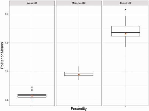
Boxplots of posterior means (n = 56 for each boxplot) of fecundity (ratio of juveniles to adults) when population abundance is 0. Fecundity was estimated by fitting RD-pop to simulated data with 10 populations and a carrying capacity of 150. Red dots are true parameter values used in simulations to generate data. The fecundity parameter used in simulations is similar to the intrinsic growth rate concept and represents a theoretical maximum when population abundance is close to 0.
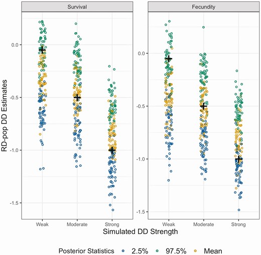
Posterior statistics of density dependence in survival and fecundity in simulated data sets with 10 populations and carrying capacity of 150. “+” sign shows the true value of the density dependence parameter used to generate the simulation set. If the “+” sign is centered on orange dots (mean of the posterior distribution) density dependence parameters in that simulation set is estimated without bias. If the “+” sign is placed around blue dots (2.5% quantile of the posterior distribution) density dependence is underestimated, or conversely if it is placed around green dots (97.5% quantile of the posterior distribution) density dependence is overestimated.
Empirical Example: Brown Creeper
We detected weak to moderate DD on survival (β = –0.27, Supplementary Material Figure S5A), and on fecundity (ζ = –0.13, Supplementary Material Figure S5B) for Brown Creeper. These DD strengths were stronger than the weak DD parameters used for simulations but weaker than the moderate DD parameters. Temporal variability was low for survival, and high for fecundity (σ s = 0.23, σ s = 0.97; Supplementary Material Table S1). Survival at mean population size for adults and juveniles were estimated at 0.42 and 0.31, respectively. Our estimate of fecundity at mean population size was 1.94 (1.21–3.01) juveniles per adult (Supplementary Material Table S1). In addition, Bayesian p-values for both the survival and fecundity components indicated good model fits (0.24 and 0.50, respectively; see a discussion of Bayesian p-values in Supplementary Material S2: Model and Simulation Details).
Projections
Density-independent projections parameterized with RD-pop fit to Brown Creeper data led to frequent population extinctions and explosions, which is apparent in the population trajectory (Supplementary Material Figure S5C) and bi-modal distribution of minimum abundances (Figure 4). Density dependence in population models led to more regularized projections in which population extinctions and explosions were less frequent (Figure 4). The distribution of minimum abundances from density-dependent projections of Brown Creeper showed a generally similar pattern to projections parameterized with RD-pop fit to simulated data irrespective of the DD strength of capture history simulations (Figure 4).
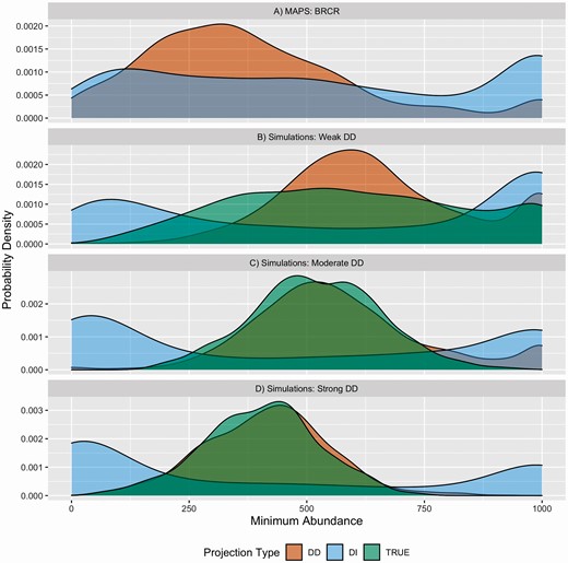
Distributions of minimum abundances resulting from population projections made with stage-structured population models that were parameterized with RD-pop fit to Brown Creeper data (A), and with RD-pop fit to simulation sets that was generated with different density dependence strengths (B, C, D). Light blue represents parameterizations of population models with density-independent (DI) RD-pop, orange represents density-dependent (DD) RD-pop, and green (TRUE) represents population models that was parameterized with original simulation parameters that was used to generate capture history data. High probability density at 0 and 1,000 indicates frequent population extinctions and explosions, respectively..
Projections made with population models that were parameterized with density-dependent RD-pop fit to simulated data were close to projections made with true simulation parameters, especially when true simulation parameters included moderate or strong DD. This correspondence demonstrates, in a biologically relevant context, the ability of RD-pop to fit realistic models to data (Figure 4C and D). In contrast, projections with density-independent RD-pop (Figure 4B–D), and with density-dependent RD-pop fit to simulated capture history data with weak DD (Figure 4B) were not close to projections with the true simulation models. Overestimation of DD strength in RD-pop fit to weak DD data also resulted in overestimation of projected minimum abundances. Density-independent projections tended to result in frequent population extinctions or explosions (Figure 4B–D).
DISCUSSION
RD-pop is a novel and useful extension of the foundational capture–recapture models. To our knowledge, RD-pop is the first capture–recapture model that uses the unique relationship among vital rates under density-dependent regulation in a single framework in order to estimate all the necessary parameters of an age-structured, density-dependent, and stochastic population model, allowing the model results to be used for medium- to long-term population forecasting. Our simulation results demonstrate that these parameters are estimated with little bias when simulation parameters are biologically realistic and capture histories can be grouped into multiple independent populations (Figures 2 and 3, Supplementary Material Figures S1–S4). Density-dependent population models created by RD-pop are ready to be used in population projections and they can produce biologically meaningful results (Figure 4). Such models are essential for conservation assessments, such as forecasting and viability analyses.
The true value of RD-pop lies in its ability to use limited data to parameterize population models that in turn can be used to predict changes in population sizes and distributions. We believe this is especially important for developing countries that do not yet have extensive bird-banding and survey programs like MAPS and BBS. For example, Turkey only has two regularly active bird-banding stations that collect robust design mark–recapture data (Nurbahar Usta, personal communication). Based on our simulation results, 10 populations for a common bird species are enough to build a useful RD-pop for population projections, if these populations are regulated with at least moderate density dependence. Funding a long-term project to increase the number of bird-banding stations so that they will represent at least 10 populations can be justifiable for funding bodies, even in a developing country. However, doing so while also establishing a country-wide bird survey program would be much harder. We believe that RD-pop provides an opportunity to do more with less in these countries if the goal is to collect data for making population projections. RD-pop also has value in its potential application to current bird-banding programs. There are more than 150 species that meet CJS model-fitting requirements in MAPS data that RD-pop can be applied to (following the criteria in Albert et al. 2016). Convergence for Brown Creeper data took ~20 hr, and this indicates majority of these species will have a feasible model run time (<1 week). For these species, RD-pop can be extended to include weather, climate effects and other exogenous factors in addition to population density.
Negative density dependence is more detectable with longer time series (Brook and Bradshaw 2006) but there are several other factors that can hinder RD-pop’s ability to provide an unbiased estimate of density dependence strength. First, any given time series needs to be variable enough so that there will be a signal of density dependence in the data; no statistical model can estimate density dependence if a population is stable around carrying capacity with very little fluctuation. In this case, RD-pop will simply give the prior back as the posterior, learning nothing new from the data. Second, density dependence strength could be low compared to environmental forcing, and without explicitly accounting for environmental variability RD-pop might mistakenly explain this variability with density dependence, leading to biased density dependence estimates. This would lead to similar results as the low density dependence strength scenario (Figures 3 and 4). Third, density dependence will also be harder to detect if populations have clear trends (increasing or decreasing) within the time frame of capture history data. In this case and the previous case, it is important to include environmental variables to account for trends so that it is easier to separate the regulating effect of density dependence (Nater et al. 2016). If the model fails to estimate a proper density dependence effect, this in turn will affect estimates of all vital rates in the RD-pop framework. Lastly, density dependence might operate on different spatial scales. Here, we modeled it on the scale of breeding populations, however for species that migrate the relevant scale might be the super-population, where individuals from different populations mix and competition throughout the nonbreeding season is not necessarily limited to individuals of the same population. In such cases, density dependence strength might be low, or slightly positive because of statistical noise.
The state of the art for estimating population size is IPMs, which model abundances as a binomial or a Poisson process (Schaub and Abadi 2011). IPMs, however, are data-hungry and require population count data in addition to mark–recapture data. In the RD-pop framework, population size is estimated as an expected value with the heuristic abundance estimator (Eq. 3). By using these expected values of population sizes, we were able to limit the data requirements of RD-pop framework to a single data source. Heuristic abundance estimators can be further improved by adding capture heterogeneity and by explicitly accounting for emigration, as is the case in many robust design studies (Kendall et al. 1995, Kendall and Bjorkland 2001, Hines et al. 2003, Kendall and Nichols 2004). RD-pop is a complex framework, however, so we kept each individual modeling component simple with lower numbers of parameters to estimate.
Vital rates are ecologically related to abundance; higher vital rates lead to higher population abundances. When both vital rates and abundance are estimated with the same data source, and abundances are used again to inform vital rates or other parameters related to vital rates, their covariance might lead to estimation issues (for example, when detecting additive mortality from harvest (Sedinger et al. 2010)). This is not the case for RD-pop, however, because density dependence simply adds circularity to the relationship between vital rates and abundance. If vital rates from time steps t to t + 1 lead to higher abundances, then higher abundance estimated in t + 1 will lead to lower vital rates in the transition from t + 1 to t + 2, and abundance will decrease in t + 2. This covariance is how density dependence is expected to occur in a population that is regulated around a carrying capacity. In the RD-pop framework, this circularity is achieved by robust design where survival is estimated in the open population part of the design and abundance is estimated in the closed part.
The survival and capture probability part of RD-pop is a Robust Design model with the addition of density and effort as covariates. Robust Design has a specific set of assumptions, especially for secondary capture occasions within primary sampling periods. Within each primary capture period, the population is assumed to be closed, there is no emigration or immigration and no births or deaths. Because we set this period to be the whole breeding season (4 months) it is likely that this assumption will be violated depending on the focal species. For example, in Brown Creeper there were only 8 juvenile captures and recaptures in May, and only 81 adult captures and recaptures in August out of a total of 3,202 across the full capture history. Some individuals may have died or left the population in a given secondary period and this would lead to a biased estimate of capture probability. This is important because capture probability is not a nuisance parameter in this framework, and we use it explicitly to estimate expected population size of adults and juveniles in a given year and population.
In our opinion, however, this type of violation of the population closure assumption is acceptable within the RD-pop framework. If capture probability estimates are biased due to the reasons explained above, they are lower than their true value. This leads to an inflated population size estimate under the heuristic population size estimator, but not necessarily to an inflated density index estimate. This is because the density index is calculated by standardizing the population size estimate of each year with the average population size across all sampling years. Any bias in population size in a given year would also be prevalent in the average population size, and therefore deviation of population size of a particular year from the average population size will not be biased to the same extent as population size estimates themselves. The population closure assumption becomes more problematic if the number of dead individuals or those leaving the population during the breeding season is not uniform across years. Then, some years will disproportionately affect the average population size estimate and will skew density estimates in other years as well. Such years can be detected with a random yearly effect term in the capture probability part of RD-pop (Eq. 2). Years with lower probability estimates than what was expected from their capture effort will be suspect to such violations. We did not include a year effect in this iteration of RD-pop because capture probability estimates of Brown Creeper were similar to estimates from previous analyses and there was no indication that population closure assumption had any significant effects in model results (See Supplementary Material S2 for comparisons with previous models).
Estimation of capture probability and survival is more likely to be an issue for juveniles than adults because of the generally low number of captures and recaptures of juvenile individuals. We address this issue by using informed priors on juvenile survival that depends on the density-dependent relationship among the 3 vital rates. Juvenile survival is determined by fecundity and adult survival, so only capture probability and residency parameters of juveniles are directly estimated by data. This relationship among vital rates provides a novel way of accounting for apparent survival rates of juveniles. For example, juvenile survival is estimated to be lower than 0.1 in a RD-pop framework when estimated without using Eq. (12) and the residency component; this is substantially lower than what was estimated with the full RD-pop framework (0.31, Supplementary Material Table S1). A higher survival estimate allows RD-pop to more confidently determine the latent state of being present and alive in a population (z), which in turn would lead to more robust capture probability estimates. This prior relationship among the vital rates, however, relies on the assumption that density dependence can be detected from capture histories of the focal species.
Dispersal tendencies and the number of captured transients of males and females can be different (Bayne and Hobson 2002), in which case sex-specific survival rates and residency parameters should be used in the RD-pop framework. If this difference between sexes is not accounted for, it will lead to biased estimates in the RD-pop framework, namely, adult apparent survival probability of residents will be lower, and because vital rates are connected this will be compensated by higher juvenile survival, lower capture probability, and higher fecundity. Here lies the inherent value of explicitly focusing on parameters with clear ecological expectations such as fecundity and density dependence. If the application of RD-pop is substantially affected by any sort of estimation bias or violations of assumptions, the estimates of these parameters will deviate from their ecological expectations. For example, fecundity of bird species can be considered within the context of a biological limit because the maximum fertility of many bird species in the world are known. If weakly informative or vague priors are used for fecundity and if its estimate is higher than this biological limit, then this would be a sign that assumptions and the structure of the RD-pop framework does not fit the data well. Similarly, density dependence can only regulate populations if it is acting negatively on vital rates with increasing population size. A “positive” density dependence would indicate a population increasing its abundance faster in every time step; this is not an ecologically realistic scenario except for allee effects which only operates when population size is low. However, if estimates are within the expectations of ecological reality, we argue that RD-pop is useful for building population models, especially if the alternative is a density-independent model or building no model at all.
ACKNOWLEDGMENTS
We thank Kevin Shoemaker for his comments and contributions. We thank the many volunteers who have contributed to the MAPS program and the Institute for Bird Populations for development and active curation of the MAPS dataset.
Funding statement: This study was initiated under funding from the NASA Biodiversity Program (NNH10ZDA001N-BIOCLIM).
Author contributions: BS and RA conceived the idea. BS developed the methods and analyzed the data. RA supervised the research. BS and RA wrote the paper.
Data availability: R and JAGS code of CJS-pop analysis, example simulation data, and results of Brown Creeper analysis are accessible at https://github.com/bilgecansen/CJS-pop. The software source code has been archived and made accessible in Zenodo (https://doi.org/10.5281/zenodo.5714788).
