


Abstract
The superior temporal and the Heschl’s gyri of the human brain play a fundamental role in speech processing. Neurons synchronize their activity to the amplitude envelope of the speech signal to extract acoustic and linguistic features, a process known as neural tracking/entrainment. Electroencephalography has been extensively used in language-related research due to its high temporal resolution and reduced cost, but it does not allow for a precise source localization. Motivated by the lack of a unified methodology for the interpretation of source reconstructed signals, we propose a method based on modularity and signal complexity. The procedure was tested on data from an experiment in which we investigated the impact of native language on tracking to linguistic rhythms in two groups: English natives and Spanish natives. In the experiment, we found no effect of native language but an effect of language rhythm. Here, we compare source projected signals in the auditory areas of both hemispheres for the different conditions using nonparametric permutation tests, modularity, and a dynamical complexity measure. We found increasing values of complexity for decreased regularity in the stimuli, giving us the possibility to conclude that languages with less complex rhythms are easier to track by the auditory cortex.
Introduction
Language related areas have been localized in studies applying positron emission tomography (PET), magnetic resonance imaging (MRI), or magneto-encephalography (MEG), as shown by extensive reviews (Klein et al. 2001; Price 2012; Chang et al. 2015; Bowyer et al. 2020). The superior temporal gyrus (STG) is known to be a critical area for speech processing, and along with the superior temporal sulcus constitute the major components of Wernicke’s area. The STG has been proposed as an interface between lower level auditory structures and higher level association areas for language-related tasks (Geschwind 1970; Buchsbaum et al. 2001; Milton et al. 2021; Bhaya-Grossman and Chang 2022). The neuroanatomical ”dual stream model” of language, which differentiates between a dorsal and a ventral pathway for processing (in agreement with visual processing theories) (Hickok and Poeppel 2004; Saur et al. 2010; Hickok 2012), supports the idea that processing of speech starts by spectro-temporal and phonological analyses in these areas. Changes in amplitude in the speech envelope are represented in the STG, as observed using high-density intracranial recordings, while participants listened to speech (Oganian and Chang 2019). Similar results were reported in Yi et al. (2019), where the authors showed that the amplitude envelope of the signal is encoded in middle to anterior parts. The authors concluded that distinct regions of the STG encode different temporal landmarks of the speech signal, yielding a functional parcellation. Moreover, the left STG is coupled to attended speech in a cocktail-party auditory scenario, as shown with intracranial EEG (Golumbic et al. 2013) and with MEG data (Vander Ghinst et al. 2016).
The process by which neural activity in the auditory cortex synchronizes with the amplitude envelope of the speech signal is known as neural entrainment. Neural entrainment captures acoustic and linguistic features such as the syllable in a frequency around 5 Hz—a syllable lasts |$\sim $|200 ms (Gross et al. 2013b)—and plays an important role in comprehension and intelligibility (Peelle et al. 2012; Doelling et al. 2014; Bosker and Ghitza 2018; Kösem et al. 2018; Poeppel and Assaneo 2020). Whether it is caused by intrinsic oscillations (Lakatos et al. 2008; Giraud and Poeppel 2012; Doelling et al. 2014; Notbohm et al. 2016; Zoefel et al. 2018) or by a sequence of evoked potentials in the theta range (Capilla et al. 2011; Keitel et al. 2014; Obleser and Kayser 2019) is still under debate, and therefore, we refer to this process simply as neural tracking.
Electroencephalography and magnetoencephalography (EEG/MEG) provide high temporal resolution measurements of the electrical activity generated by thousands of cortical pyramidal cells activated simultaneously in the brain (Niso et al. 2022). Due to its high reliability in real-time applications, they are popular technologies for experiments on language (Peelle and Davis 2012; Gross et al. 2013a, b; Doelling et al. 2014; Vander Ghinst et al. 2016; Assaneo and Poeppel 2018; Kösem et al. 2018; Zoefel et al. 2018). The elevated cost and restricted availability of MEG has favoured the use of EEG, which provides lower signal-to-noise ratio (SNR) and lower spatial resolution. EEG measurements result from a superposition of several sources in sensor (electrode) space, and the generators of potentials and fields cannot uniquely be reconstructed without further constraints (Hämäläinen and Ilmoniemi 1984; Keil et al. 2014), rendering a precise localization impossible (Van Rullen et al. 2011; Henry et al. 2014; Kayser et al. 2015; di Liberto et al. 2015; Henry et al. 2016; Bonhage et al. 2017; Ding et al. 2017; Broderick et al. 2018; Van Bree et al. 2021). Localization accuracy is affected by, among others, head-modelling errors, source-modelling errors, and EEG noise (Grech et al. 2008; Wendel et al. 2009).
Different source reconstruction procedures have been proposed to find the sources in the brain that is responsible for the measured potentials at the EEG electrodes, that is to find an estimated solution to the inverse problem (Hallez et al. 2007). Although several guidelines and recommendations have been published, the applied methodologies are quite specific for each particular study and there are no universal prescriptions for localization of sources and more importantly, for how to analyze and interpret them (Will and Makeig 2011; Keil et al. 2014; Diessen et al. 2015; Michel and Brunet 2019; Cox and Fell 2020; Niso et al. 2022). For instance, the authors in Xie et al. (2022) propose a pipeline to perform cortical source reconstruction with high-density EEG data and realistic MRI models, and then a parcellation of reconstructed activities into brain regions of interest (ROIs) for major brain lobes or brain networks. However, the aim of the pipeline is to analyze resting-state functional connectivity by computing the FC between each pair of ROIs. In the present work, we present a general pipeline to analyze oscillatory signals in source space. The feasibility of this approach has been tested by analyzing EEG data measuring neural entrainment to different languages.
In a recent study, we measured neural tracking to resynthesized sentences from Japanese, Spanish, and English—each corresponding to three different linguistic rhythms: mora, syllable, and stress, respectively—in two different population of listeners: natives of Spanish and natives of English (Özer et al. 2023). The goal of this research was to investigate how different linguistic rhythms impact native language neural processing. Linguistic rhythm is associated with syllabic complexity, that is with the variability of the syllable duration (see Box 1). One methodological advantage of this study was the use of resynthesized sentences that preserved all prosodic and syllabic complexity of the original sentences while removing meaning (see Ramus and Mehler (1999) for a description of the resynthesis method). The reason for choosing resynthesized speech was to remove top-down components (i.e. meaning) in participants speech processing. To evaluate the differences between the three rhythmic conditions (mora, syllable, stress), we computed phase-locking value (PLV) between stimuli and EEG measurements in the theta frequency band (|$\sim \! 5$| Hz). PLV results showed lowest values to stress (the least regular rhythm in terms of syllabic complexity), intermediate to syllable, and highest values to mora. The trend was the same in both groups—English and Spanish natives—showing that there was no impact of native language in neural tracking. The increasing trend in the PLVs in both groups matched the ordering in decreasing syllabic complexity of the stimuli, giving us the possibility to conclude that languages with less complex rhythms are easier to track.
Linguistic rhythm is based on the beat of the speech signal fluctuates on: feet, syllables, or morae. World languages have been classified according to their rhythm into stress-timed, syllable-timed, and mora-timed (Ramus and Mehler 1999; Ramus et al. 1999; Langus et al. 2017; Abercrombie 2022). Stress-timed languages such as English have a wide variety of syllables, from standalone vowels (V) (e.g. a) to complex strings of vowels and consonants (C) (e.g. strict: CCCVCC), yielding a high variability in syllable duration. Syllable-timed languages would represent the intermediate case with medium variability (e.g. Spanish). On the other extreme, mora-timed languages allow few syllabic structures such as V, CV (consonant-vowel) and in a restricted way also CVC (e.g. Japanese), yielding a low variability in syllable duration. In summary, stress-timed languages would correspond to highest syllabic complexity and highest variation in syllable duration, syllable-timed would be the intermediate case with medium syllabic complexity and medium variation in syllabic duration, and mora-timed languages would correspond to lowest complexity and lowest variation.
The present work presents a procedure for analysis and interpretation of source reconstructed data, which has been tested with the data just described. We started with a time–frequency analysis of EEG prior to projection of sensor data into standard Montreal Neurological Institute (MNI) space. Note that this is not a critical step, as the nonfiltered time-series can also be projected directly. Source reconstruction was performed using functions adapted from the Matlab-based MEG/EEG Toolbox of Hamburg (METH, Guido Nolte) and custom-made scripts. The ICBM-152 template head model, an MRI database of young adult brains using data from 152 subjects (aged 18.5–43.5 years) acquired as part of the International Consortium for Brain Mapping (ICBM database) (Mazziotta et al. 1995), and realistic positions of the sensor locations, were used to compute lead field matrices (see Materials and methods and Fig. 1A). We then performed a priori statistical comparisons between the source projected power time-series belonging to the different conditions by means of nonparametric permutation tests with maximum statistics. We focused on the signals in the STG including the Heschl’s gyrus (HG)1 and found behaviour in the data that could evidence a functional parcellation (Hickok 2012; Ozker et al. 2017; Yi et al. 2019; Li et al. 2021). To identify exactly which voxels were contributing to each subarea, we performed a Louvain community analysis (Blondel et al. 2008; Rubinov and Sporns 2010) and reordered the entries in the space dimension matching the found communities, coinciding roughly with the anterior (aSTG), the medial (mSTG), and the posterior (pSTG) parts of the STG in both hemispheres. Due to the oscillatory nature of the differences we found with the statistical tests, we considered an analysis of the signals using the well-known dynamical Lempel-Ziv (LZ) measure of complexity (Lempel and Ziv 1976; Ziv and Lempel 1978) (see Materials and methods and Fig.1B). Our results show that the distribution of LZ complexity measures from the left STG exhibits an ordered pattern that parallels the syllabic complexity hierarchy present in the stimuli. In other words, we observe lowest LZ complexity for lowest syllabic complexity (mora) and highest LZ complexity for highest syllabic complexity (stress), with a strong effect for English natives on the left hemisphere. We do not observe the same trend either in the right STG or in other areas of the brain. The results for power values show a different trend, with both groups exhibiting highest power for syllable, intermediate to mora and lowest to stress. The differences are observed mostly in the medial and posterior parts of the STG. In all conditions, the power for the Spanish participants is higher than for the English ones.
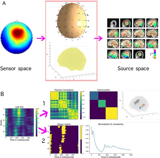
(A) Visualization of power time-series projection to source space (left column). Sensor level signals are projected using a standard MNI model and realistic positions of the electrodes (middle column). The |$xyz$| coordinates of the 3D grid correspond to values in the axial, sagittal, and coronal planes, respectively. The resulting matrix has power values in MNI space (right column), where we display changes relative to mean power, here expressed in arbitrary units (a.u.). (B) Matrix of power time-series in left STG (49 voxels |$\times $| 50 time points). (1) Visualization of the community detection process: Pearson correlation of the time-series (49|$\times $|49 matrix), the three communities detected and the corresponding 49 voxels in STG showing the functional parcellation (the voxels of the right STG are also highlighted in black color for visualization purposes). (2) Graphical representation of the normalized LZ complexity computation: binary matrix obtained by thresholding the signals with 1 SD and the evolution in time of the LZ measure in time, normalized by its entropy at each time instant.
To discard possible confounds in the modularity analysis results, caused by neighboring effects in the application of inverse methods, we generated synthetic data by computing the forward model in three different controlled scenarios. The found potentials at sensor space were subject to the same analysis as the original empirical data. The results of the simulations shed light on how the modularity analysis operates and allowed us to discard that a functional parcellation in the STG could be caused by the nature of the inverse method.
Materials and methods
Participants
The data were collected and preprocessed as reported in Özer et al. (2023). Twenty-four English-native adults (aged 23.71|$\pm $|4.07) participated in Experiment 1 (M = 8, F = 16), and 24 Spanish-native adults (aged 23.17|$\pm $|4.74) participated in Experiment 2 (M = 9, F = 15). The participants were assigned to the groups according to the language they grew up speaking to their parents, regardless of the accent or country of origin. English speaking participants did not have a broad knowledge of other languages, and especially Spanish or Japanese, and they had not spent more than 6 months in a Spanish speaking country. Sample sizes were decided in accordance with other studies studying neural entrainment to speech, e.g. Peña and Melloni (2012), Pérez et al. (2015). All participants reported right-handedness and no hearing problems. They signed an informed consent before starting the experiment and were paid 20 euros for their participation. The experimental procedures were approved by the Drug Research Ethical Committee (CEIm) of the IMIM Parc de Salut Mar, reference 2020/9080/I.
Stimuli
Stimuli consisted of 100 Saltanaj resynthesized sentences in Dutch and English (stress-timed languages), Spanish and Catalan (syllable-timed languages), and Japanese (mora-timed language), 20 in each language (Ramus and Mehler 1999). The phoneme durations and pitch curves were preserved as they are in the original sentences (Ramus 2002). Then, the phonemes were replaced by their linguistic equivalents (i.e. phonemes that are common to most languages): all fricatives are replaced with /s/, vowels with /a/, liquids with /l/, stop consonants with /t/, nasals with /n/, and glides with /j/ (Ramus and Mehler 1999). With this method, the English sentence “The next local elections will take place during the winter” is transformed into “sa natst latl alatsans jal taat tlaas tjalan sa janta.” More examples of the Saltanaj resynthesized sentences can be found online (http://www.lscp.net/persons/ramus/resynth/ecoute.htm).
EEG data acquisition and preprocessing
EEG was recorded at 1,000 Hz with online high-pass filtering over 0.1 Hz via a 64-channel Acticap on BrainVision Recorder and BrainAmp amplifier (Brain Products, Germany). Channel distribution was in accordance with the extended international 10–20 system. Event marker triggers were sent via MatLab during the recording. One channel was placed on the nose as the online reference, as well as two outer channels on the left and right mastoid bones to be averaged offline. Finally, two channels were placed horizontally and vertically next to and under the right eye, respectively, in order to record eye movements and blinks. Impedances were kept below 10 k|$\Omega $|.
Data preprocessing was conducted on MatLab using Fieldtrip toolbox (Oostenveld and Praamstra 2001). Independent component analysis was implemented on continuous EEG signals to identify and eliminate heart and eye movement artifacts. Then, continuous data were segmented into trials by delimiting 1 s before and 3.5 s after the sentence onset to match the longest duration of stimulus sentence. Power line frequency was removed from each epoch and the signals were rereferenced to the mastoidal channels. Noisy channels and trials were visually detected and eliminated. Channels that were eliminated and those deemed noisy were interpolated using spherical spline algorithms to the neighbouring channels by triangulation. Then, a time–frequency analysis was performed using Morlet wavelets, with a frequency resolution of 0.25 Hz and a time resolution of 50 ms (from |$-1$| s to 3.5 s from onset), resulting in a 2D matrix for each trial. The frequency band of interest was |$f\ =\ [4.75,6.5]$| Hz, chosen after identification by visual inspection of changes in amplitude direction |$\sim $|5 Hz.
Source reconstruction
Source reconstruction of EEG signals was performed using functions adapted from the Matlab-based MEG/EEG Toolbox of Hamburg (METH, Guido Nolte) and custom-made scripts, following a procedure similar to the one in Pfeffer et al. (2018).
Lead field matrices
Since anatomical information from the individual subjects was not available, leadfield matrices were computed using an MNI template head model and realistic positions of the sensor locations (Nolte and Dassios 2005). The 3D grid consisted of M=5,003 voxels and was constructed from the ICBM152 template (Fonov et al. 2011), covering grey matter of the entire brain and keeping an approximate distance of 7.5 mm between neighbouring points (Baillet and Garnero 1997; Pascual-Marqui 2002). This is in accordance with the standards in Baillet and Garnero (1997) and Brinkmann et al. (1998), which state that spatial and temporal accuracy should be at least 5 mm and 5 ms, respectively. Finally, realistic 3D positions of a 64-sensor configuration were obtained from published work (see link) and adapted to our particular layout (Oostenveld and Praamstra 2001).
Spatial filters
Sensor signals from |$N\! =\! 60$| nodes were projected into the 3D grid by means of the dynamic imaging of coherent sources (DICS) method (Gross et al. 2001). Four electrodes were used as references and therefore excluded. The DICS is similar to a linearly constrained minimum variance beamformer filter (van Veen et al. 1997), but relying on the cross-spectrum density matrix (frequency domain) rather than on the signal covariance (time domain). We computed spatial filters specifically for each subject in the frequency band |$f=[4.75,6.5]$| Hz using the average cross-spectrum |$C\in \mathbb{C}^{N\times N}$| computed across trials and conditions (mora, syllable, stress). The subject-frequency-specific filter |$A\in \mathbb{R}^{M\times N\times 3}$| for every voxel |$m$| in the grid was computed as
where |$L_{m}\in \mathbb{R}^{N\times 3}$| is the |$m$|th entry of the leadfield matrix |$L\in \mathbb{R}^{M\times N\times 3}$|. In (1), we used the real part of |$C$|, previously regularized to avoid inversion problems by letting |$C=C+\alpha I$|, where |$I$| is the identity matrix and |$\alpha \,=\,0.05*\mathrm{trace}(C)/N$| (Gross et al. 2001). The dipole orientation chosen for each voxel corresponded to the value of the maximum singular value |$s$| of the matrix |$A_{m}^{T} C A_{m}$|, so that the filter |$A_{1}\in \mathbb{R}^{N\times M}$| had entries |$A_{1_{m}} = A_{m}u_{1}$|, where |$u_{1}\in \mathbb{R}^{3}$| is the left singular vector associated with |$s$|.
Source projection and z-scoring
For each time-point, unbiased source-level cross-spectral density estimates were obtained from the sensor-level cross-spectral density matrix |$C$|, and the unbiased spatial filter |$A_{1}$|, to compute the power vector of estimates as follows |$p = \text{diag}(A_{1}^{T} \operatorname{Re}\{C\} A_{1})$|. The obtained source space data vector was further corrected with the beamformer noise power map. Due to the relatively low SNR, noise spatial spectrum may exceed the spatial spectrum of the neural activity of interest, an effect known as the ”center of head” bias. In order to reduce this problem, a normalization of the estimated spatial spectrum with estimated noise spatial spectrum is performed. The obtained measure is the neural activity index, a measure that can be interpreted as an estimate of the source to noise variance (van Veen et al. 1997; Sekihara and Nagarajan 2008; Westner et al. 2022). The resulting data matrix (power vectors for all time points) was finally z-scored using the time-window [|$-500,-200$|] ms before stimulus onset (Cohen 2014), where mean and SD values were averaged across trials and conditions for each subject.
Data analysis
Statistical analyses
Analyses were performed on the normalized z-scored power signals from the STG. Whereas there are 49 voxels in the MNI grid labeled as left STG, there are 71 labeled as right STG (4 and 6, respectively, correspond to HG). Therefore, the data matrices had dimensions 49/71|$\times $|40|$\times $|24|$\times $|3 (space, time in intervals of 50 ms, subjects, and conditions). The three conditions were compared pairwise in the frequency band of interest. A priori comparisons were carried out for (i) the 4D matrix of power time-series and (ii) the vectors of mean power across time, both in the interval 500–2500 ms, using nonparametric permutation tests with maximal statistics, avoiding thus the multiple-comparisons problem (Nichols and Holmes 2002).
Functional community detection
In most trials, we observed homogeneous activity for roughly three groups of voxels, which corresponded mainly to the aSTG, mSTG, and pSTG in both hemispheres (see Fig. 1B1), in agreement with previous reported findings on functional parcellation in the STG (see, e.g. (Hickok 2012; Ozker et al. 2017; Yi et al. 2019; Li et al. 2021)). To identify exactly which voxels in the grid were contributing to each subgroup, we performed a Louvain community analysis (Blondel et al. 2008; Rubinov and Sporns 2010). Communities are groups of nodes within a network that are more densely connected to one another than to other nodes. The metric modularity evaluates how much more densely the nodes are connected within a community compared with how connected they would be, on average, in a random network. We found three communities on the left hemisphere and three on the right hemisphere using the Louvain community algorithm applied to the Pearson correlation matrix (gamma = 1.1), (see Fig. 1B1). The rows of the data matrices were then reordered according to the community they belonged to on average. In the left hemisphere, we assigned 15 voxels to the anterior part, 13 to the medial, and 21 to the posterior STG. In the right hemisphere, the distribution was 18 for the anterior, 36 for the medial, and 17 for the posterior STG.
Normalized Lempel Ziv complexity
Due to the oscillatory nature of the signals, we considered comparing the conditions using a dynamical measure of complexity. The most popular one is algorithmic complexity, and a practical implementation of this theoretical idea was proposed by researchers Lempel and Ziv (see Box 2).
Introduced by Kolmogorov (1965), algorithmic complexity is defined as the number of bits of the shortest algorithm (e.g. computer program) capable of reproducing a given symbol sequence. LZ complexity measures how diverse the patterns present in a particular signal are. Whereas regular signals can be characterized by a small number of patterns and yield low LZ complexity, irregular signals require longer dictionaries and yield a high LZ complexity. Thus, a signal is regarded as complex if it is not possible to provide a compressed representation of it. The LZ complexity is computed in three steps: first, the signal is binarized; then, the binary sequence is scanned sequentially to look for distinct patterns or structures, building up a dictionary that summarizes all the sequences. The length of this dictionary, or equivalently, the number of patterns found, defines the LZ complexity.
We computed the LZ complexity in two steps: (i) binarization of the time-series by reducing the signal to a spatio-temporal point process: select the time points at which the signal crosses a threshold equal to 1 SD and set them to one, and zero elsewhere, introducing thus a Poincaré section. The Poincaré section is a threshold independent procedure that decreases the dimension of the phase space and consequently the size of the data sets, facilitating further numerical investigations, as shown by Tagliazucchi et al. (2012). We performed the same binarization for all the signals in the STG, yielding a 2D matrix for each trial (voxels |$\times $| time). (ii) Spatio-temporal computation of the LZ complexity following the procedure in Casali et al. (2013): let |$SS(x,t)$| denote the binary matrix with |$x = 1,\dots ,M$| and |$t = 1,\dots ,T$|, the indices of the spatial and temporal dimensions, respectively. The algorithm runs through the first column of |$SS(x,t)$| (space) searching for patterns. The search is repeated for each subsequent column (time) while keeping track of patterns encountered in previous columns (see Fig. 1B2). Let |$L$| stand for the total number of spatio-temporal samples, |$L = M\times T$|, and let |$l(t_{1})$| be the number of samples of |$SS(x,t)$| up to a time |$t_{1}$|, |$l(t_{1}) = M\times t_{1} $|. The LZ complexity is then normalized by the source entropy of the signal, given by
where |$p_{1}$| is the number of “1s” contained in the binary sequence of length |$l(t_{1})$|. At each time |$t$|, the algorithm calculates a number |$c_{l}(t)$| that corresponds to the normalized LZ complexity of the bi-dimensional sequence of length |$l(t)$|. In this way, we obtain a |$T$|-long vector for each trial. It is important to notice that, if the signals have not changed significantly from one time point to the next one, something expected as we deal with continuous oscillations, no drastic change in the number of words of the dictionary is expected. In this way, space-information is taken into account and preserved.
Boxplots to visualize the distribution of median values were generated with the python function boxplot, which uses Gaussian-based asymptotic approximation to the binomial distribution to compute the confidence intervals (whenever the notch parameter is set to true). The upper and lower bounds for the confidence intervals were computed analytically using the expression |$nq \pm z\sqrt{nq(1-q)}$| rounded up to an integer, where |$n$| is the sample size, and |$q$| is the quantile interest, which for 90% confidence for the median are |$q\!=\!0.5$| and |$z\!=\!1.645$| (Conover 1999).
Simulated data
To validate the results, we used synthetic data generated with a forward calculation to obtain the potentials at sensor space. We then performed the same inverse calculations and analyses applied to the original empirical data. For consistency, we simulated data for the same amount of subjects and 30 trials per condition and considered three different scenarios where the signals were generated at the STG. In the first scenario, a unique dipole with |$xyz$| coordinates |$d_{1}\!=\![-6.75, -2.25, 0.75]$| (in cm) and momentum |$m_{1}=[-0.9560, 0.0166, -0.2930]$| with an associated oscillation in the theta frequency band was activated in the medial part of the STG. In the second one, three dipoles with their corresponding oscillations were activated in the posterior, medial, and anterior parts of the STG, respectively, with coordinates |$d_{1}$|, |$d_{2}\!=\![-6, 0, -1.5]$|, and |$d_{3}\!=\![-6,-3.75, 2.25]$| and momenta |$m_{1}$|, |$m_{2}\!=\![0.6252, 0.3304, 0.7071]$|, and |$m_{3}\!=\![-0.6161, -0.4250, -0.6631]$|. In the third scenario, all dipoles in the STG were activated with an associated oscillation. Precise information about the momenta of the dipoles was obtained from the volume conductor model included in the METH toolbox. To keep the signals as close as possible to the real ones, the oscillations were obtained as the average of two time-series randomly selected from a set of trials belonging to the same condition and subject, but from a different voxel source, although still belonging to the STG. In other words, the original source reconstructed time-series were randomized across the voxels (space dimension) and circularly shifted by a random amount in the time dimension before averaging. Finally, white Gaussian noise was added at sensor space. This procedure was repeated 30 times for each subject and condition to keep the simulation as close as possible to the real data. The sensor space data from the three different scenarios were analyzed using the same pipeline as the one applied to the original empirical data.
Results
For the comparison between power time-series belonging to different conditions, we computed the average across trials for each condition, that is data matrices had dimensions |$49\times $|40 and 71|$\times $|40 (voxels |$\times $| time points) for left and right hemispheres, respectively, and then performed the nonparametric permutation tests with maximum statistics. We excluded the first 500 ms after stimulus onset to isolate the effect of evoked potentials (Zoefel and VanRullen 2016). Since these were a priori statistical comparisons, we considered that a significant difference was detected when the |$P$|-value was below |$0.05$|.
Within-group Spanish sample
The results for the Spanish participants are shown on the top row of Fig. 2. Column A shows the average power across voxels and subjects along with the SD calculated across subjects for the left aSTG. Significant differences were found at 2,100 ms and 2,150 ms from stimulus onset in the left aSTG (mora > stress) as shown by the |$P$|-value map in column B. For visualization purposes, column C shows the subgroup the voxel belongs to in MNI space. Note that, although only the subgroup where the difference was found is shaded, the comparisons were made on the entire STG.
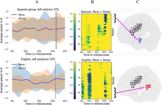
Top row: results for the Spanish participants. (A) Mean power in theta range in the anterior STG, averaged across subjects and trials. (B) |$P$|-value map for the comparison mora > stress. (C) voxel localization in MNI space. Bottom row: results for the English participants. (A) Mean power in theta range in the in the posterior STG, averaged across subjects and trials. (B) |$P$|-value map for the comparison mora > stress. (C) Subgroup the voxel belongs to in MNI space.
To compare the mean power across time, trial information was preserved, so that data matrices had dimensions 49/71|$\times $|trials for each condition. Nonparametric permutation tests show no significant differences between conditions in either hemisphere. Kruskal–Wallis tests show differences in the distributions of means. This means that the differences across conditions vanished when computing the means across time.
Within-group English sample
The results for the English participants are shown on the bottom row of Fig. 2. Column A shows the power averaged across voxels and subjects along with the standard deviationSD (calculated across subjects) for the left pSTG. English participants show significant differences in the left pSTG (mora > stress), as shown by the |$P$|-value map in column B. Differences in the left mSTG can be also observed, although not achieving statistical significance (not highlighted). As before, column C shows the subgroup the voxel belongs to in MNI space, but the comparisons were made on the entire STG.
Trial information is again preserved to compare the mean power across time. Nonparametric permutation tests show significant differences for the mean (mora > stress) in two voxels in the left STG (|$P$|-values |$0.0266$| and |$0.0341$|), and one in the right STG (syllable > stress, |$P$|-value |$0.0323$|).
Between-group comparisons
Power time-series
Significant differences were found for the three conditions in the a priori comparisons between groups for the power time-series only in the left STG, as shown in Fig. 3. A: Mora, two voxels in mSTG show significance (|$P$|-values |$0.0246$|, |$0.0420$|, |$0.0325$|), 1,350–1,400 ms. B: Syllable, one voxel in pSTG shows significance (|$P$|-value |$0.0432$|) at 1750 ms. C: Stress, two voxels in pSTG show significance (|$P$|-values |$0.0489$|, |$0.0333$|, |$0.0475$|) at 900–950 and 2,150 ms. Remarkably, Spanish group exhibits systematically larger values of power than the English group. Mean across time does not show differences neither in the left nor in the right STG.
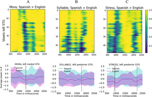
Top row: |$P$|-value map for the comparisons between groups yielding in all cases, Spanish > English. Bottom row: average power and SD across subjects, voxels, and trials for left mSTG and left pSTG.
Normalized LZ complexity
To compute the normalized LZ complexity measure |$c_{l}(t)$|, we binarized the spatio-temporal matrices and computed |$c_{l}(t)$| at every time point |$t$| (see Materials and methods). Since complexity reduces with time (see Fig. 1B2), i.e. as we increased the length of the binary sequence, we considered all the time points from stimulus onset (|$t = 0$|–|$2,500$| ms) to capture the expected decrease and compare the distributions across conditions.
The top row of Fig. 4 shows the median values (highlighted horizontal lines) of the distribution of complexity values and their 0.90 confidence interval (highlighted vertical lines) for A: the Spanish group and B: the English group. The number of points for each boxplot is |$43,500, 43,050,$| and |$43,550,$| respectively, for the Spanish group and |$43,900, 44,250,$| and |$42,250,$| respectively, for the English group. The variation is due to a different final number of trials for each condition and subject.
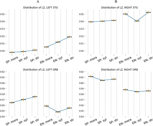
Top row: median values and CI intervals (vertical lines) for the distribution of |$c_{l}(t)$| values for both groups in the STG in (A) the left and (B) the right hemisphere. A clear increasing pattern is observed only in the left hemisphere. Bottom row: median values and CI intervals for the distributions of |$c_{l}(t)$| in the superior frontal gyrus (medial orbital) cortex (ORB) in (A) the left and (B) the right hemisphere.
We can observe a weaker increasing trend in the median values of the Spanish group compared with those of the English group. Comparing all the distributions, Kruskal–Wallis test gives |$P=0.0024$| for the Spanish group, and |$P = 1.2$| e|$^{-26}$| for the English group. Comparisons between groups (English vs. Spanish), Kruscal–Wallis test yields |$P = 1.3$| e|$^{-73}$|, meaning that all the distributions differ. Pairwise comparisons within groups yield:
Whereas the comparison mora vs. stress shows the largest gap, the differences in median are not significant for mora vs. syllable in both groups. For the sake of completeness, we computed the LZ complexity also in the right STG and in an area not directly related to early stages of language processing: the superior frontal gyrus medial orbital cortex (ORB). The LZ complexity for the signals in left and right STG is depicted on the bottom row of Fig. 4. We observe that the clear increasing trend is no longer observed for English natives in the right hemisphere (B) and remains weakly increasing but still not significant different for Spanish natives (A). On the other hand, the increasing trend is preserved in the ORB area for the Spanish natives, as observed in the bottom row of Fig. 4. Interestingly, the right hemisphere (B) exhibits larger values of LZ complexity for both the STG and ORB. In summary, comparing the medians of the distributions, the signals in the left STG exhibit lowest complexity as compared with the right STG or to the ORB in both hemispheres. The signals for the Spanish group exhibit always lower complexity than those from the English groups.
Modularity analysis on synthetic data
A modularity analysis was performed on the synthetic data using the same parameters for the three different scenarios. For the single dipole, the homogeneity and uniformity of the reconstructed signals does not lead to a detection of communities, which is an expected result. The three dipole scenario gives rise to a more varied situation in which the algorithm is able to find two communities. However, the distribution of communities differ, separating inner and outer voxels, i.e. in their deepness with respect to the cortex. This could be caused by two dipoles pointing in the inner direction, while the other one is pointing in the outer direction, indicating that the signals from the formers are merged. Finally, the third scenario assumes that the sources have independent noncorrelated signals in the entire STG, which would constitute an extreme case. For this final scenario, the modularity analysis returns the finding of up to four communities, but with a different ordering as shown in Fig. 5. Notice that none of the simulated situations are realistic, as the activity of the rest of the brain is not considered. However, these highly controlled scenarios help us discard the hypothesis that the functional parcellation observed in the empirical data can be caused by the inverse method itself.
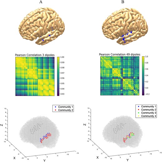
Top row: dipole localization and momentum directions for two simulated cases: (A) three active dipoles and (B) 49 active dipoles. Middle row: visualization of the community detection process: Pearson correlation of the synthetic time-series for the two cases detecting (A) two communities and (B) four communities. Bottom row: precise localization of the voxels belonging to each community in the simulated scenario.
Discussion
This work presents a novel approach for analysis and interpretation of source reconstructed signals from data collected with EEG. Due to the high temporal resolution of the measurements, EEG and MEG have been widely used in speech and language-related experiments. However, localization of sources using EEG has to be treated with caution, since measurements result from a superposition of signals in sensor space, rendering a uniquely reconstruction of the generators impossible (Wendel et al. 2009; Vatta et al. 2010). Despite these limitations, source projected signals still exhibit a more than acceptable accuracy, and we propose a methodology for their analysis showing that reliable results can be obtained. In a nutshell, our method starts by comparing projected space-time signals belonging to different conditions by means of nonparametric permutations tests with maximum statistics, followed by a modularity analysis to identify functional clusters and to regroup the signals according to the community they belong to. Finally, the LZ complexity measure is computed to assess differences between conditions. The approach was tested on data from an experiment on perception of linguistic rhythm in which we measured neural tracking to resynthesized sentences from Japanese (mora-timed language), Spanish (syllable-timed), and English (stress-timed) in two different populations: natives of Spanish and natives of English (Özer et al. 2023). Differences in perception were expected due to variations in the duration of the syllable in a frequency |$\sim $|5 Hz. Therefore, for the present study, we started with a time–frequency analysis of the signals in sensor space, and after projection onto source space, we concentrated on the signals from the STG and the HG in the theta frequency band.
Source reconstruction was carried out using functions adapted from the Matlab-based MEG/EEG Toolbox of Hamburg (METH, Guido Nolte) and custom-made scripts. The toolbox includes several spatial resolutions for the grid, with a minimum of 624 and up to a maximum of 16,873 voxels, that is, with an intervoxel distance ranging from 1 cm to 0.5 cm. This is a sensitive choice that may have a great impact on the results (Baillet and Garnero 1997; Pascual-Marqui 2002; Grech et al. 2008; Wendel et al. 2009). Our selection of medium-dense grid of 5,003 voxels with an intervoxel mean distance of 0.75 cm yielded consistent results, as shown by the outcome of the modularity analysis that revealed a functional parcellation, in alignment with previously reported studies (Hickok 2012; Ozker et al. 2017; Yi et al. 2019; Li et al. 2021). Inverse calculations were computed by means of beamformers with the cross-spectral density matrices method DICS. The DICS has been widely used in research and clinical applications (Gross et al. 2001; Jaiswal et al. 2020) and it has the advantage that it can be applied to time–frequency-transformed data and it can find coherence for evoked and induced activity in a predefined time–frequency range.
Nonparametric permutation tests with maximum statistics (Nichols and Holmes 2002), avoiding thus the multiple comparisons problem, led to the identification of entries in the space–time data matrices (voxels) showing statistically significant differences. Although this is not a critical step in the analysis, it provides information that may be relevant to select areas of interest in the brain before carrying out any comparison between conditions. A Louvain community analysis with parameter gamma = 1.1 (Blondel et al. 2008; Rubinov and Sporns 2010) revealed a functional parcellation with three main communities, which coincided approximately with the anterior (aSTG), the medial (mSTG), and the posterior (pSTG) parts of the STG in both hemispheres. Simulated data of highly controlled scenarios have helped us realize that these communities cannot be caused by the inverse method. Indeed, in the three dipole scenario, we observed that two communities where found, rather than three. We speculate that it might be caused by two dipoles having momenta pointing in a similar direction in their activation. The 49 dipole scenario, where there was no structural organization in space and time revealed that, although the algorithm is able to detect up to four communities, and this could be caused by the regularity in time, the localization of the communities is not homogeneous and does no coincide with the ones observed in the empirical data.
Due to the oscillatory nature of the signals, we evaluated the differences between conditions by computing the dynamical LZ measure of complexity at every time instant (see Materials and methods). Our results show that the distribution of LZ from the STG and HG in the left hemisphere exhibit an ordered pattern that resembles the classification of variability in syllabic duration of the stimuli. In other words, we observe lowest LZ complexity for lowest variability in syllabic duration (mora) and highest LZ complexity for highest variability in syllabic duration (stress), with a strong effect for English natives on the left hemisphere. This trend is consistent in the entire left STG and HG and should not be surprising, since low variability in syllable duration translates into less variability in the distance between peaks (vowels) in the sound pressure wave, yielding simpler dictionaries in the binary signal and thus lower LZ complexity. On the other hand, the opposite should be true for higher variability in syllabic duration, as the interpeak distance has larger variance. The authors in Henry et al. (2014) proposed that rhythm reduces the complexity of high-dimensional neural dynamics and suggest that the use of rhythm as a means to organize neural oscillations reduces the complexity of neural phase effects on behaviour. We do not find the increasing trend in complexity neither in the right STG for the English group nor in other areas of the brain, as shown by the results from the superior frontal gyrus (medial orbital) cortex, an area not directly related with language, although for the Spanish group is still weakly observed in the left hemisphere. Moreover, a different trend is observed for power values, since both groups exhibit highest power for syllable in mean over time, intermediate to mora and lowest to stress. These differences in power are observed mostly in the medial and posterior parts of the STG. According to the authors in Yi et al. (2019), posterior STG might be sensitive to speech onset following a period of silence (200 ms or longer), whereas middle-to-anterior STG may track peaks in the amplitude envelope of continuous speech.
Although we tested our methodology on data from a language-related experiment, we believe that it can be easily applied to other paradigms and believe that it would be interesting to test it in experiments for which other areas of the brain have to be considered. The choice of diverse partitions of the 3D grid would then be corroborated applying the nonparametric permutation test followed by the modularity analysis we have proposed. The communities found thereby would give information on how to regroup the data in the space dimension accordingly and eventually on how to adjust the parameters, such as the gamma parameter of the Louvain algorithm that controls for the number of communities found. This is a crucial step before computing the spatio-temporal complexity measure.
Complexity of neural data has been analysed using several measures of structural and dynamical complexity, such as symbolic dynamics derived from time-series (Atay et al. 2009), information fluctuation (Bates and Shepard 1993), or order patterns (Schinkel et al. 2012) to name a few (Wackerbauer et al. 1994). LZ complexity has been applied to EEG measurements in studies on epilepsy (Radhakrishnan and Gangadhar 1998), anaesthesia (Zhang et al. 2001; Puglia et al. 2021), altered states of consciousness (Schartner et al. 2017), and also to fMRI (Casali et al. 2013; Boly et al. 2015; Varley et al. 2020), fNIRS (Liang et al. 2022), and MEG (Shumbayawonda et al. 2018). Binarization of the signal is required for the computation of the LZ measure, and in our case, we applied it to signals in a narrow frequency band. A possible drawback for broadband or nonfiltered signals is that the resulting binary signal could generate dictionaries with a very large number of symbols or patterns, yielding nonsignificant differences between conditions. Given the nature of the proposed method, it could be interesting to apply it in the time-dimension, e.g. for the analysis of evoked potentials. One important advantage is that it can be applied to any type of data provided they consist of oscillatory signals, without the need of filtering them a priori, although the latter could be a convenient step in most situations.
We have shown that a modularity analysis followed by the computation of the dynamic LZ complexity can be applied to successfully characterize signals from source space when focusing on a narrow frequency band, yielding the possibility of distinguishing between conditions. The advantages of our methodology are manifold since the tools applied are available, easily to use, and the implementation of the computations is straightforward. Moreover, it allows for the possibility of considering alternative complexity measures that could better adapt to signals of diverse characteristics.
Conclusion
We have proposed a methodology for analysis and interpretation of source reconstructed signals from EEG measurements, when signals belonging to different conditions have to be evaluated and compared. The method, which relies on a sequence of simple computations, has been tested on data from a language-related experiment and has shown reliable results. Starting from signals in sensor space, we focus on a predefined frequency band before projection onto source space, compare conditions by means of nonparametric permutation tests with maximum statistics in the areas of interest, and then perform a modularity analysis followed by a reordering of the data according to the identified communities. Finally, a comparison between conditions is performed by means of the normalized dynamic LZ complexity measure.
Acknowledgments
The authors would like to thank Dr Thomas Pfeffer, Prof. Guido Nolte, Dr Yonatan Sanz Perl, and Prof. Gustavo Deco for insightful discussions and suggestions for the improvement of this work.
Funding
This research was supported by grants from the Spanish Ministry for Science and Innovation (Project PID2021-123416NB-I00 financed by MCIN/ AEI/ 10.13039/501100011033 / FEDER, UE), by the Economical and Social Research Council (ESRC) (ES/S010947/1, UK), and from Institució Catalana de Recerca i Estudis Avançats (P-5993 ICREA Acadèmia 2018) awarded to NSG. EEO was supported by the Catalan Government (2021 FI B2 00123 ID Q5850017D).
Footnotes
For simplicity, in the following, we refer to the accumulated voxels from both areas as STG.
References