


Abstract
Mounting evidence suggests that transcranial alternating current stimulation can enhance response inhibition, a cognitive process crucial for sustained effort and decision-making. However, most studies have focused on within-session effects, with limited investigation into the effects of repeated applications, which are crucial for clinical applications. We examined the effects of repeated bifocal transcranial alternating current stimulation targeting the right inferior frontal gyrus and pre-supplementary motor area on response inhibition, functional connectivity, and simulated driving performance. Thirty young adults (18–35 yr) received either a sham or transcranial alternating current stimulation (20 Hz, 20 min) across 5 sessions over 2 wk. Resting-state electroencephalography assessed functional connectivity between the pre-supplementary motor area and right inferior frontal gyrus at baseline, the final transcranial alternating current stimulation session, and the 7-d follow-up. Response inhibition was measured using a stop-signal task, and driving performance was assessed before and after the intervention. The results showed significant improvements in functional connectivity in the transcranial alternating current stimulation group between sessions, though response inhibition and driving braking performance remained unchanged. However, while not the targeted behavior, general driving performance potentially improved following bifocal transcranial alternating current stimulation, with participants maintaining stable driving behavior alongside increased spare attentional capacity. These findings suggest that repeated bifocal transcranial alternating current stimulation may enhance cortical connectivity and related cognitive-motor processes, supporting its potential for clinical applications.
Introduction
Executive function is a set of higher-order cognitive processes that enable goal-directed behavior, problem-solving, and adaptive responses to novel or complex situations (Blair 2016). One of the key components of executive function is response inhibition, which plays a vital role in the continuous monitoring, adapting, and updating of behaviors in response to changes in the environment (Mostofsky and Simmonds 2008). Impaired response inhibition has been linked to various psychological disorders characterized by impulsive behavior, including addiction, attention deficit hyperactivity disorder, obsessive compulsiveness, and eating disorders (Lipszyc and Schachar 2010; Smith et al. 2014; Bartholdy et al. 2016). Specifically, maladaptive response inhibition often manifests as slower execution of stopping responses or a diminished ability to delay the initiation of behaviors compared to healthy controls (Schmitt et al. 2018).
Response inhibition is also particularly important in everyday tasks requiring sustained effort and decision-making, such as driving, where safe driving often requires the inhibition of prepotent responses (Hatfield et al. 2017; Adrian et al. 2019), and where distractions can lead to catastrophic consequences (Beanland et al. 2013; World Health Organization 2015). Considering the essential role of response inhibition in daily functioning and its identification as a core deficit in multiple psychological disorders, it is crucial to develop effective strategies to enhance response inhibition. Such advancements could pave the way for new intervention techniques that improve the quality of life and safety for those experiencing issues related to response inhibition (Bari and Robbins 2013).
Understanding the neural mechanisms of response inhibition is crucial for improving its functionality. Key regions involved include the right inferior frontal gyrus (rIFG, the pre-supplementary motor area (preSMA), and the subthalamic nucleus, forming a cortical network essential for inhibitory control (eg Aron and Poldrack 2006). Imaging studies have shown associations between successful inhibition in stop-signal tasks (SSTs) and increased activation in the rIFG and preSMA (eg Dambacher et al. 2014; Erika-Florence et al. 2014; Hampshire et al. 2010; Simmonds et al. 2008; Tsvetanov et al. 2018). Furthermore, transcranial magnetic stimulation (TMS) studies support the causal role of these regions, showing that the disruption of the rIFG or preSMA during stop trials impairs inhibitory control (Obeso et al. 2013; Allen et al. 2018).
Notably, a body of research suggests that the rIFG and preSMA work together to transmit neural signals through the basal ganglia to the primary motor cortex, effectively suppressing and canceling motor response. Studies using functional magnetic resonance imaging (fMRI) have revealed extensive functional connections between the rIFG and pre-SMA during response inhibition, with both regions interacting with the basal ganglia (Jahfari et al. 2012). While some suggest that only the preSMA directly connects to the basal ganglia (Duann et al. 2009; Coxon et al. 2012; Rae et al. 2015), evidence supports robust connectivity between the rIFG and preSMA, particularly during successful inhibition (Jahfari et al. 2012; Dambacher et al. 2014; Rae et al. 2015). TMS findings reveal that disrupting preSMA affects the influence of the IFG on motor output (Neubert et al. 2010), and enhancing preSMA activity strengthens connectivity within the fronto-basal-ganglia circuit (Xu et al. 2016). These results underscore the critical role of rIFG-preSMA connectivity in response inhibition, offering potential targets for enhancing inhibitory control.
One technique that has the potential to improve the functional connection between the rIFG and preSMA is transcranial alternating current stimulation (tACS) (Antal and Paulus 2013). tACS is a noninvasive neuromodulation technique that applies weak oscillating electrical currents to the scalp. This technique is believed to affect the rhythmic activity of the brain by aligning endogenous neural oscillations with the frequency of the applied stimulation (Herrmann et al. 2013). When tACS is administered concurrently to 2 distinct cortical areas (ie bifocal tACS), it has the potential to enhance functional connectivity and communication between the stimulated regions. Polanía et al. (2012) provided empirical evidence that bifocal tACS can modulate functional connectivity between cortical regions during a working memory task. Using 0° relative phase (in-phase) and 180° relative phase (antiphase) stimulation over the left prefrontal and parietal cortices, they found that in-phase stimulation improved working memory performance, whereas antiphase stimulation decreased performance. These findings suggested that tACS may influence the phase alignment of endogenous oscillations within frontoparietal networks that are essential for working memory. For response inhibition, our previous study (Fujiyama et al. 2023) demonstrated that in-phase bifocal tACS at a beta frequency (20 Hz) over the rIFG and preSMA enhanced response inhibition and strengthened task-related functional connectivity, as observed with EEG. Similarly, other studies have reported favorable effects of bifocal tACS on a variety of cognitive and motor functions (eg Violante et al. 2017; Reinhart and Nguyen 2019; Grover et al. 2022; Meng et al. 2023; Lebihan et al. 2025).
While these findings highlight the potential of tACS to improve inhibitory function, most studies to date only examined its effect within a single session using unifocal tACS. An exception is a study conducted by Grover et al. (2022), who applied repeated unifocal tACS over 4 d and observed a positive impact on working memory, yet changes in functional connectivity were not considered in their study. It is, therefore, important to establish whether changes in functional connectivity and related improvements in cognitive function (behavior) are retained over an extended period, which is a crucial attribute of any clinically meaningful intervention. Notably, no existing research has investigated whether multiple sessions of bifocal tACS over the rIFG and preSMA can result in long-lasting effects on functional connectivity and response inhibition.
The current study, for the first time, investigates whether bifocal tACS can induce lasting changes in functional connectivity between the rIFG and preSMA and improve response inhibition over an extended period of 7 d. In addition, we explored the effects of repeated bifocal tACS application over the rIFG and preSMA on response inhibition. In addition to measuring the effect of stimulation on SST performance in a laboratory setting (Congdon et al. 2012), we extended our investigation to a real-world task requiring inhibition—simulated driving. This approach allowed us to evaluate the broader applicability of bifocal tACS and assess whether improvements in inhibitory control could extend to more complex, everyday tasks. We chose driving as it relies on executive functioning, including response inhibition (Hatfield et al. 2017; Adrian et al. 2019). Specifically, drivers need to sustain attention and appropriately allocate sufficient cognitive resources to control their vehicle, navigate to a destination, and respond to hazards, which often requires inhibition of prepotent responses. Distraction, which occurs when attention is captured by other tasks, such as mind-wandering (Albert et al. 2022), looking at an engaging billboard (Crundall et al. 2006), or by a mobile phone (Gariazzo et al. 2018), can also lead to significant driving performance decrements. As resisting distraction has been linked with response inhibition (Bissett et al. 2017), enhancing response inhibition could potentially improve driving performance and safety. By investigating the effects of bifocal tACS on both lab-based response inhibition tasks and simulated driving, we aim to bridge the gap between controlled experimental settings and real-world applications. This approach allows us to assess the potential of tACS as a tool for improving cognitive functions critical for everyday activities, particularly those requiring sustained attention and inhibitory control.
Method
Participants
All potential participants underwent screening for contraindications to noninvasive brain stimulation (NiBS) and driving tasks, with exclusions made for individuals with psychiatric or neurological conditions or those taking medications incompatible with the stimulation protocol (Rossi et al. 2021). Handedness was assessed using the Edinburgh Handedness Inventory (Oldfield 1971), and only participants who scored above 40, indicating right-handedness, were included in the study. This criterion was based on evidence linking left-handedness to variations in motor cortical representations and differing aftereffects of NiBS (Nicolini et al. 2019; Fitzgerald et al. 2021). Prior to their participation in the study, all participants provided written informed consent. This study was approved by the Murdoch University Human Ethics Committee (2020/186).
A power analysis to estimate the required sample size was performed using the “simr” package (Lenth 2020) in the R statistical package, version 4.4.1 (R Core Team 2024), drawing on simulation data from our previous studies investigating the effect of NiBS on behavioral measures (Fujiyama et al. 2016, 2022). With an alpha level set at 0.05 and a target power of 0.90, we estimated that 32 participants would be sufficient to detect a medium pre-post tACS change in response inhibition within a group (Cohen’s d = 0.4) based on a study that captured medium to large effect sizes on working and long-term memory task performances following multiple tACS sessions (Grover et al. 2022). Estimating an ~ 20% attrition rate (Lansbergen et al. 2007), we recruited an additional 8 participants, resulting in a total of 40 participants.
Of the 40 participants recruited via the Murdoch University Research Participant Portal, 4 withdrew from the study due to scheduling conflicts, and one withdrew due to motion sickness after the first driving session. As a result, the current study started with 35 participants (Meanage = 23.16, SDage = 4.89 yr, 26 females). After the first tACS session, 2 participants dropped out due to scheduling conflicts. Two additional participants withdrew for the same reason after the third session, and 1 other participant did not return after the fourth session for undisclosed reasons. This resulted in 30 participants (Meanage = 23.29, SDage = 3.65 yr, 21 females) completing all 5 tACS intervention sessions. For follow-up (FU) assessments, 1 participant in the tACS group did not complete the 7-d FU due to a scheduling conflict, resulting in 29 participants (Meanage = 23.33, SDage = 4.54 yr, 20 females) completing all sessions. To address missing data, we did not use case-wise deletion. Instead, we included all available data at each time point in the analysis by employing a linear mixed-effects model, accommodating missing observations. Nevertheless, the results should be interpreted with some degree of caution due to the attrition rate and the reduced sample size at FU.
Participants were pseudo-randomly allocated to either the tACS or sham group to maintain balance as recruitment progressed. Allocation was adjusted iteratively to ensure an approximately equal number of participants in each group while accounting for ongoing recruitment dynamics. Consequently, both groups had 15 participants (10 female) with similar age profiles (tACS = 24.27 yr, sham = 22.69 yr, P = 0.53), noting that one of the participants in the tACS group did not participate in the 7-d FU. Informed consent was obtained prior to participation in the experiment.
Materials
Stop signal task
Response inhibition was measured using an SST, a task that is considered a valid measure of latent response inhibition (Congdon et al. 2012). PsychoPy version 1.90.3 (Peirce et al. 2019) was used to program an 80-trial 2-option reaction time (RT) SST program on a computer with a monitor refresh rate of 144 Hz. As illustrated in Fig. 1, each trial began with a white fixation cross presented in the center of a black screen, which was then presented for 500 ms. Subsequently, an imperative go signal (green arrow indicating left or right) was displayed, prompting the participant to press the corresponding arrow on the computer keyboard using their right index finger as fast as possible. Participants were instructed to start each trial by placing their index finger on the downward arrow key, which is situated between the left and right arrow keys, to avoid biased responses. RT was measured between the onset of the go signal (green arrow) and the registration of the button press. Visual feedback was presented for all go trials, with RT presented in milliseconds on the screen after each successful go trial, “wrong response” for an incorrect response, and “missed” for no response. In 25% of the trials, the green go signal was followed by a stop signal (red arrow) facing the same direction as the green go signal, which prompted participants to withhold their initiated response. The stop signal delay (SDD)—the time between the onset of the go signal and the stop signal—was manipulated in a staircase fashion (Verbruggen et al. 2019) across all blocks with an initial SSD of 200 ms and a minimum SSD of 50 ms. SSD increased by 50 ms in the subsequent trial for every successful stop, while SSD decreased by 50 ms in the subsequent trial for every failed stop signal response (Aron and Poldrack 2006; Allen et al. 2018). Visual feedback was given, with “good!” presented for every successful stop and “try to stop” following every failed stop to encourage participants to perform their best.
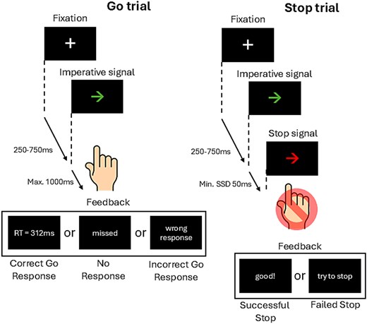
Schematic illustration of a trial sequence in the SST. Participants were instructed to respond to an imperative go signal (green left- or right-pointing arrow) using their right index finger by pressing the corresponding key on a computer keyboard. Participants kept their index finger on the down arrow key on the keyboard between trials to avoid biasing the response. During stop trials (25% of the total trials), where the previously presented green arrow would turn red after a dynamic delay (SSD), participants had to withhold their response. SSD on the subsequent stop trial was increased or decreased by 50 ms following successful or unsuccessful stopping, respectively.
Driving simulator tasks
The medium-fidelity driving simulator used Oktal’s SCANeR Studio software (version 1.4) and featured 3 parallel 27-inch monitors mounted within an Obutto cockpit, providing a 135° wide-field display. Figure 2 shows the front windscreen view displayed on the central monitor, including a digital speedometer and a central rear-view mirror. Participants sat approximately 85 cm away from the central monitor and operated a right-hand-drive vehicle using a Logitech steering wheel and pedal set. Vehicle speed and position data were recorded continuously at 1,000 Hz and down-sampled to 50 Hz for analysis.
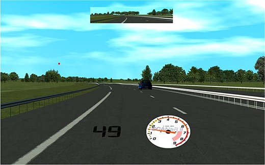
The central monitor view of the driving environment with rear-view mirror and digital speedometer displayed. A DRT target is presented above the horizon on the left.
For the main (targeted) driving task used to assess response inhibition, participants completed a 10-min braking task based on Muhrer and Vollrath (2011; also see Facchin et al. 2023). The braking task required participants to react as quickly as possible to an external event to change their routine driving behavior. Participants were instructed to follow a lead car traveling at 50 km/h on a straight section of road while maintaining a safe following distance (Fig. 3). The lead car was programmed to brake 8–11 times over a 3 km distance. One lead car braked predictably (ie every 20 s) before turning off the road. The participant then followed a second lead car, which subsequently braked unpredictably (20–40 s between braking events). The order of lead car presentation was counterbalanced.
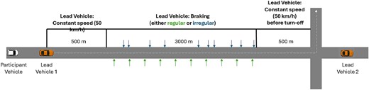
Braking task schematic. The participants followed a lead vehicle for 500 m at a constant speed before the lead vehicle started braking either regularly or irregularly. Once lead vehicle 1 turned off the main road, the participant encountered lead vehicle 2. The braking process was identical for lead vehicle 2, except for the pattern of braking, which was alternated (eg if lead vehicle 1 braked regularly, then lead vehicle 2 braked irregularly).
For generality, we also assessed fundamental vehicle control abilities. Participants drove in the inside right lane of a continuous 4-lane road, which was free of traffic, while the remaining lanes had light traffic (~5 vehicles per minute). During a 5-min practice scenario, participants were instructed to drive as close to the 50 km/h speed limit as possible while remaining in their lane. Participants then drove for ~20 min.
While driving, participants also completed a visual detection response task (DRT; Jahn et al. 2005). As illustrated in Fig. 3, this task required them to respond to peripherally presented red dot targets (0.34° of visual angle) that appeared on the central monitor within an area 2° to 4° above the horizontal midline and 11° to 23° to the left of their forward viewpoint (Patten et al. 2006). Targets remained visible for up to 2 s or until a response was made. Subsequent targets were separated by 6–16 s. Participants responded to targets by pressing a button on the steering wheel with their right thumb, ensuring their hands stayed on the wheel (Martens and Van Winsum 2000; Bowden et al. 2017, 2019). Participants were instructed that driving safely was their primary task, and responding to the DRT stimuli was a secondary task.
Participants’ speed and accuracy in responding to DRT targets can be considered as a measure of their spare cognitive capacity, thereby providing an immediate and quantifiable measure of the latent “cognitive workload” (Castro et al. 2019; International Standards Organization, ISO DIS 17488 2016) being used by participants to maintain fundamental vehicle control. Specifically, faster RTs and/or higher accuracy indicate greater spare cognitive capacity, reflecting the cognitive resources available beyond the primary driving task (Castro et al. 2023; International Standards Organization, ISO DIS 17488 2016).
Electroencephalography
Electroencephalography (EEG) was recorded using a 128-electrode EEG HydroCel Geodesic Sensor Net (Magstim EGI, Eugene, OR). Net Station (5.4.2) software recorded sensor-level EEG signals from Ag-AgCl scalp electrodes. Signals were amplified using a Net Amps 300 amplifier and low- and high-pass filtered (0.1–500 Hz) with a 1,000 Hz sample rate. Electrode impedance was kept below 50 kΩ as recommended by the manufacturer (Magstim EGI, Eugene, OR). During resting-state EEG (rsEEG) recording, participants viewed a fixation cross presented on a PC monitor for 3 min.
tACS
Bifocal tACS was administered using the neuroConn DC-STIMULATOR MC machine (NeuroConn, Ilmenau, Germany). Three rubber electrodes of 2 cm in diameter were applied to the scalp using Ten20 conductive paste in a 2 × 1 montage (Fig. 4), targeting the rIFG and preSMA. The electrode placement was determined using the international 10–20 system. The preSMA was located at Fz, and the rIFG was in the intersection between Fz to T4 and Cz to F8. Alternating currents were applied using a beta frequency of 20 Hz. A current intensity (peak-to-peak amplitude) of 1 mA was applied to the rIFG and 1.6 mA to the preSMA with zero DC offset, which was informed by the e-field modeling presented elsewhere (Tan et al. 2020).
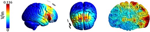
Electrical current flow modeling for the tACS (2 × 1) electrode montage over the rIFG and preSMA (adapted from the importance of model-driven approaches to set stimulation intensity for multi-channel tACS, by Tan et al., published in Brain Stimulation, 2019, under a CC BY 4.0 license. Vol75 (mesh volume with field strength ≥75% of the 99.9th percentile) and Vol50 (mesh volume with field strength ≥50% of the 99.9th percentile) provide measures of focality. The gray circles represent the rubber electrodes (2 cm diameter) with 2 active electrodes placed anteriorly and one return electrode placed posterior to the target region. The current amplitude (1 mA peak-to-peak) was equally split between the 2 active electrodes.
The currents were delivered using a 0° phase to the preSMA and rIFG, indicating that the peaks and troughs of the electrical waves were coupled in both regions. The stimulation was sustained for 20 min, a period chosen to allow sufficient time for the neural circuits to respond to the electrical modulation (De Koninck et al. 2023). In the sham condition, the tACS stimulation ramped up to the respective current intensity and immediately ramped down at the beginning and end of the 20 min for 30 s to simulate stimulation (Woods et al. 2016). The tACS machine was pre-programmed by a research associate with codes representing the 2 conditions to ensure both participant and researcher blinding.
Control measures
Sleep, Caffeine, and Alcohol Questionnaire. The Sleep, Caffeine, and Alcohol Questionnaire (SCA-Q) (eg Fujiyama et al. 2023) was used to account for potential confounding factors affecting the response to tACS, such as sleep quality, hours slept, and caffeine and alcohol consumption within the 12 h prior to the session. Sleep quality was rated on a scale from 1 (poor) to 10 (excellent). Participants reported caffeine consumption in milligrams and alcohol consumption in standard drinks, with reference tables provided to help accurately estimate the caffeine content of various beverages and the standard drink equivalents of alcoholic beverages.
Transcranial Electrical Stimulation Questionnaire. Upon completion of each tACS session, a Transcranial Electrical Stimulation (tES) Questionnaire (Vancleef et al. 2016; Fujiyama et al. 2022, 2023) was given to assess blinding adequacy and stimulation effects. The questions involved the sensations experienced and the side effects of the stimulation. The questionnaire includes 12 items of sensations that are commonly associated with NiBS, such as “heat,” “headache,” and “tingling” (Woods et al. 2016). The items were rated on a 5-point Likert scale, ranging from “nothing” to “very strong.” The same rating scale was used to ask participants whether the sensations affected their performance of the SST, ranging from “a little” to “very much.” Furthermore, 3 items were asked about the time the sensations occurred during the stimulation with a 3-point Likert scale, comprising “at the start”, “in the middle”, and “at the end” of the stimulation.
Procedure
The project timeline for each participant was consistent across both active and sham groups (Fig. 5). Participants completed 5 experimental sessions of either active or sham tACS, followed by a 7-d post-intervention FU session. rsEEG was conducted during the first (baseline) and fifth (post-intervention) sessions. During rsEEG recording, participants were instructed to maintain a neutral gaze at a fixation cross for 3 min (eyes open), avoiding complex thought processes. Following the rsEEG, participants completed the SST during EEG recording. This began with a 16-trial practice session, followed by 2 blocks of 80 trials (pre-stimulation). tACS electrodes were then applied using conductive paste, and stimulation was administered for 20 min, including a 30-s ramp-up and ramp-down. During stimulation, participants completed 3 additional blocks of 80 SST trials (mid-stimulation). After the tACS session, another rsEEG recording was conducted, followed by 2 additional blocks of SST trials. The EEG nets remained in place during the tACS application, as the tACS electrodes were applied without needing to remove the nets. Subsequent experimental sessions (sessions 2–5) consisted only of the 20-min tACS application and 3 blocks of 80 SST trials. While both resting-state and task-related EEG data were collected, this study focuses on rsEEG to examine baseline neural oscillatory activity. This aligns with the primary objective of exploring the effects of repeated tACS application on behavior and functional connectivity.
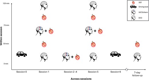
Project timeline within and across sessions. Participants received tACS over 5 sessions (sessions 1–5) across a 2-wk period, with 1–2 d between each session. rsEEG was recorded in sessions 1 and 5, as well as during FU sessions at 7 d post-intervention. Driving task performance was assessed in session 0 (baseline) and session 6 (post-intervention). In sessions 1–5, participants performed the SST during tACS application. Additionally, in sessions 1 and 5, the rsEEG and SST were administered both before and after tACS to examine within-session effects. During the FU sessions, the SST was performed without tACS.
The 7-d FU session included EEG recordings and 2 blocks of the SST. The first and fifth sessions lasted approximately 90 min, while the remaining sessions were around 45 min each. Driving performance was assessed at session 0 (prior to the tACS intervention) and 1 d after the final tACS session (session 6). The decision to separate the post-intervention driving assessment from the EEG and stop signal RT (SSRT) assessments was primarily due to logistical constraints. The tACS, EEG, and SST assessments were conducted at the Murdoch University campus, while the driving task was administered at the University of Western Australia campus. Given the need for specialized facilities and equipment at each location, it was impractical to perform all assessments at the same site.
Data processing and statistical analysis
EEG pre-processing
EEG data were pre-processed using the EEGLAB toolbox RELAX (Bailey et al. 2023) through the MATLAB environment (MathWorks, R2023b). RELAX is a data-cleaning pipeline that reduces vascular, ocular, and myogenic-induced artifacts to preserve neural signal readings. Using RELAX, the data were down-sampled at 500 Hz. Then, a 50 Hz notch filter and a bandpass filter (1–80 Hz) were applied. Second, problematic EEG sensors and noisy time periods were removed. Third, eye blink and muscle movement-induced artifacts were removed using the Multiple Wiener Filtering method. The wavelet-enhanced independent component analysis removed artifacts not detected in the previous method. Last, once the removed EEG sensors and artifacts were interpolated, the data were divided into 2-s segments for statistical analysis.
Functional connectivity between the rIFG and preSMA regions was measured using the imaginary coherence (ImCoh), which measures the consistency of phase differences between 2 signals (Nolte et al. 2004). Unlike the real part of coherency, the imaginary component is insensitive to artifacts caused by volume conduction (Nolte et al. 2004). Larger ImCoh values represent stronger phase synchrony between the 2 cortical areas, indicating the presence of a specific temporal relationship (Cattai et al. 2021). For ImCoh calculation, the time series of each electrode were convolved with complex Morlet wavelets for frequencies between 4 and 90 Hz in 1 Hz increments (87 wavelet frequencies in total). The length of the wavelets started at 3 cycles for the lowest frequency and logarithmically increased as the frequencies increased, such that the length was 13 cycles for the highest frequency. This approach balances temporal and frequency precision (Cohen 1988). To minimize the effects of edge artifacts, analytic signals were obtained from time windows of 400 to 1,600 ms (at 20 ms intervals) within each 2,000 ms epoch. ImCoh values at 20 Hz were computed for each epoch using an electrode cluster centered on Fz and AFz to represent the preSMA and a cluster consisting of FC6, F6, and F4 to represent the rIFG using the following formula: |$\left| Imaginary\ \left(\frac{S_{ij}(f)}{\sqrt{S_{ii}(f){S}_{jj}(f).}}\right)\right|$|
Here, |$i$| and |$j$| represented the time series of each electrode. For frequency |$f$|, the cross-spectral density |${S}_{ij}(f)$| was taken from the complex conjugation of the complex Fourier transforms |${x}_i(f)$| and |${x}_j(f)$|. Coherency was extracted by normalizing the cross-spectral density by the square root of the signals’ spectral power, |${S}_{ii}(f)$| and |${S}_{jj}(f)$|. ImCoh values range from 0 to 1, where a value of 0 indicates completely random phase angle differences between the signals, while a value of 1 signifies perfect phase coupling between them.
SST calculation
The integration method (Verbruggen et al. 2019) was used to calculate SSRT, which served as a measure of response inhibition (ie action cancellation when the stop signal appears). The integration method is less affected by stopping success rates that deviate from 50% (Band et al. 2003). Specifically, for each participant and at each time point, the mean SSD was individually computed. In the initial stages of calculating the SSRT, all go trials were considered. This comprehensive approach included go trials where choice errors occurred, as well as those with premature responses, ensuring a thorough representation of the participant's performance across various trial types (Verbruggen et al. 2019). Since SSRT estimation relies on the assumption of an independent race between the go and stop processes (eg Verbruggen and Logan 2009), for each participant and each assessment time point, we excluded conditions if the mean RT on unsuccessful stop trials was greater than the mean Go RT in that same condition (Verbruggen et al. 2019). Furthermore, for each participant and for each time point, conditions with stop accuracy < 0.25 or > 0.75 were excluded, as suggested by Congdon and colleagues (2012) and Verbruggen et al. (2019). Go RT for correct responses in the corresponding trials was arranged in ascending order, and the Go RT corresponding to the stop success rate (ie 1% successful inhibition) was identified. For example, if the stop success was 55%, the 55th percentile Go RT was identified as the quantile RT, and the mean SSD was subtracted from the quantile RT to estimate SSRT. We also excluded SSRTs less than 50 ms from the statistical analyses (Congdon et al. 2012). For Go RT analysis (but not for the calculations of SSRT), any trials with less than 150 ms of Go RT were excluded as they were deemed to be too fast (Perquin et al. 2024).
Driving task data processing
For the braking task, performance was only recorded during the braking interval (Fig. 2), which excludes the constant speed interval in which participants accelerated to match the lead vehicle speed. We recorded speed variability (km/h) and time headway (THW) between the participant car and the lead car THW = separation/speed). THW during braking events indicates how participants adapted their behavior to the lead car braking, with a larger headway allowing them to react more safely to braking events (Muhrer and Vollrath 2011).
For the general driving task, the first 45 s of driving were excluded to allow participants to accelerate. We then recorded speed and lane position variability (lower variability reflects improved speed/lane maintenance), median speed (km/h), and time spent speeding (>5 km/h over the limit, a commonly perceived threshold for our Australian driving participants; Bowden et al. 2017). For the DRT, a DRT hit was recorded if participants responded within 2.5 s of target onset, and a DRT false alarm was recorded for responses made outside this window. Median RT to hits is reported (correct DRT RT).
Statistical analysis
A generalized linear mixed model (GLMM) was constructed to analyze ImCoh and dependent variables for the driving task, while a linear mixed model (LMM) was employed for SSRT. For ImCoh and SSRT, 2 models were constructed. First, we constructed a model that analyzed the within-session effect of tACS. For this model, the fixed factors of GROUP (tACS and sham), TIME (pre and post), and SESSION (session 1 and session 5) were included for ImCoh, and for SSRT, an additional level in TIME (pre, during, and post) was included in the model. Second, for a model that analyzed between-session effects examining the effect of repeated tACS application, the fixed factors of GROUP (tACS and sham) and SESSION (session 1, session 5, and 7-d FU) for ImCoh and an additional 3 levels in SESSION (session 1, session 2, session 3, session 4, session 5, and 7-d FU) for SSRT were included in the model using pre-stimulation data for each session, while for the driving tasks, the fixed factor SESSION had only 2 levels: Session 0 and session 6. Within-session changes in SST and ImCoh data from sessions 1 and 5 were analyzed to evaluate the effects of tACS. For SST, the model included fixed factors of GROUP (tACS and sham) and TIME (pre, during, and post). For ImCoh, the model used the same fixed factors, but TIME included only 2 levels (pre and post). For the GLMMs analyzing ImCoh, data at the single-trial level were used to maximize statistical sensitivity. This approach avoids ecological bias inherent in averaged coherence values while allowing mixed-effects models to explicitly separate within-participant temporal variability (via random intercepts) from systematic between-participant effects, consistent with recommendations for neurophysiological time-series analysis (Chen et al. 2021; O’Connell et al. 2022). Additionally, for SSRT, we examined changes in response inhibition performance during the application of tACS across 5 stimulation sessions. For all models, the by-subject intercept was included as a random effect.
The assumptions for the models, including linearity, homogeneity of variance, and normal distribution of the model’s residuals, were evaluated using the “DHARMa” package (Hartig 2024), which employs a simulation-based method to examine residuals for fitted G/LMMs. Null hypothesis significance testing for main effects and interactions was conducted using Wald chi-squared tests for the GLMM analyses and F-tests for LMM analyses, and significant main effects and interactions were further investigated using Bonferroni-corrected contrasts where appropriate. To avoid potential misinterpretations and oversimplifications of the outcomes (Pek and Flora 2018), standardized effect sizes for each fixed factor were not reported for the GLMM. To facilitate the interpretation, Cohen’s d for FU contrasts was provided alongside significance levels. Mann–Whitney tests were used to assess differences between the groups in sleep duration, sleep quality, and caffeine and alcohol consumption at each session, while Wilcoxon’s signed-rank tests were used to assess differences between sessions for each group separately. For both Mann–Whitney and Wilcoxon’s signed-rank tests, r value was provided as a measure of effect size for each comparison. Statistical significance for all tests was set at 0.05. In presenting results, the data were expressed as mean ± 95% confidence intervals, unless specified.
Statistical analyses and visual illustrations were performed using the R statistical package, version 4.4.1 (R Core Team 2024) with an integrated environment, RStudio version2024.04.2 + 764 (RStudio Team 2015) for Windows using “lmerTest” v3.1–3 (Kuznetsova et al. 2020) to fit LMM and GLMM, and “DHARMa” package (Hartig 2024) for LMM assumptions of linearity, homogeneity of variance, and normal distribution of residuals “emmeans” v1.10.3 (Lenth 2024) for FU contrasts, “ggplot2”3.5.1 package (Wickham et al. 2016) for graphical plots, “dplyr” v1.1.4 (Wickham et al. 2023) for data manipulation, “janitor” v2.2.0 (Firke 2023) for cleaning data, “here” v1.01 (Muller and Bryan 2020) for declaring paths, “knitr” v1.47 (Xie 2024) for report generation, “reader” v1.0.6 (Cooper 2017) for reading data files, “reshape2” v0.8.1 (Wickham 2007) for reshaping data, “skimr” v2.1.5 (Waring et al. 2022) for data summaries, “stringr” v1.5.1 (Wickham 2023) for string operation wrappers, and “coin” v1.4–3 (Hothorn et al. 2023). All data and codes are publicly available on the Open Science Framework: https://osf.io/bdy4q/.
Results
Control measures
Descriptive and inferential statistics for SCA and tES sensation ratings are shown in Table 1. Mann–Whitney tests revealed that there were no statistical differences between the tACS and sham groups in sleep quality and duration, consumption of caffeine or alcohol, or sensation related to tACS in any sessions, suggesting a limited impact of the confounding factors on outcome measures and that participants were likely blinded from the conditions.
Comparisons between the tACS and sham groups on sleep quality and duration, consumption of caffeine and alcohol, and sensation related to tACS.
| tACS | Sham | |||||
|---|---|---|---|---|---|---|
| M | SD | M | SD | P | r | |
| Sleep quality (0–10) | 6.93 | 1.62 | 7.15 | 1.35 | >0.31 | <|.23| |
| Sleep duration (h) | 7.47 | 1.23 | 7.12 | 1.24 | >0.38 | <|.22| |
| Caffeine consumption (units) | 37.55 | 38.95 | 29.53 | 52.62 | >0.26 | <|.25| |
| Alcohol consumption (units) | 0.46 | 1.54 | 0 | 0 | >0.09 | <|.20| |
| tES sensation (0–62) | 10.03 | 5.39 | 7.93 | 5.48 | >0.17 | <|.28| |
Descriptive statistics are averaged across sessions for each group. The smallest P-value and the largest absolute r-value across tests that compared group differences at each session are presented. tES, transcranial electrical stimulation.
Similarly, for each group, Wilcoxon’s signed-rank tests revealed no statistically significant differences between sessions on sleep quality and duration, caffeine and alcohol consumption, and sensations related to the stimulation, ps > 0.42, |rs| < .28. This indicated that sleep quality and duration, consumption of caffeine and alcohol, and sensation related to the stimulation were comparable across sessions within groups.
EEG functional connectivity (ImCoh)
Within-session changes. None of the main effects and interactions were statistically significant, χ2 < 0.69, ps > 0.42, suggesting that ImCoh did not change within sessions 1 or 5 for either group.
Between-session effect. There was a significant main effect of SESSION, χ2 (1) = 45.66, P < 0.001 and interaction between GROUP and SESSION, χ2(2) = 139.89, P < 0.001. As shown in Fig. 6, ImCoh in the tACS group showed a significant increase from session 1 to session 5, rising by 5.4%, z = 5.58, P < 0.001, d = 0.69. This improvement was maintained at the 7-d FU, where ImCoh was 3.9% greater than at session 1, z = 3.52, P = 0.001, d = 0.48. In contrast, ImCoh in the sham group significantly declined from session 1 to session 5 by 6.9%, z = −5.74, P < 0.001, d = 0.83, and a further 7.4% reduction from session 5 was observed at 7-d FU, z = −6.12, P < 0.001, d = 0.96. The group differences were evident across all 3 sessions; at session 1, the tACS group had a significantly lower ImCoh value than the sham group, z = − 2.67, P = 0.008, d = 0.79, while at session 5 and 7-d FU, the tACS group had greater ImCoh values than the sham group, zs > 2.39, ps < 0.017, ds > 0.74.
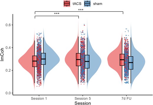
ImCoh changes across sessions for the tACS and sham groups. The boxplots show the median and interquartile range to visually summarize central tendency and dispersion. The horizontal line within the box plot represents the median. The top and the bottom lines represent the upper and lower quartiles, respectively. The data points outside of the whiskers are >1.5 quartiles. Asterisk (*) denotes a statistically significant change within the group. The tACS group showed a statistically significant increase in ImCoh from session 1 to session 5, and the increase was maintained at the 7-d FU. ***P < 0.001.
Stopping ability (stop signal RT)
Within-session changes. Contrary to the expectation, neither GROUP x TIME nor GROUP x TIME x SESSION interactions were statistically significant, Fs < 0.48, ps > 0.61, suggesting that tACS did not have an impact on SSRT within session 1 or 5. The only significant effect was the main effect of SESSION, F (1, 360.43) = 9.28, P = 0.003, indicating that, overall, SSRT was significantly faster in session 5 (205.79 ± 4.01 ms) than in session 1 (222.05 ± 3.64 ms). No other main effects and interactions were significant, Fs < 2.60, ps > 0.08.
During-session changes. To investigate the SSRT changes during the application of tACS, we examined the differences in SSRT performance during tACS between sessions 1–5. A significant main effect of SESSION, F(4, 447.65) = 2.73, P = 0.03, and FU contrasts revealed that SSRT during stimulation at session 1 (218.53 ± 8.77 ms) was faster than session 5 (235.42 ± 9.16 ms), t = 3.14, P = 0.02, d = 0.17. Importantly, the interaction between GROUP and SESSION was not statistically significant, F(4, 447.65) = 1.55, P = 0.19
Between-session changes. We observed a significant main effect of SESSION, F(5, 545.27) = 3.32, P = 0.006. As illustrated in Fig. 7, the FU contrast showed that SSRT at 7-d FU (216.25 ± 7.51 ms) was significantly faster than sessions 2 (228.44 ± 7.80 ms) and 4 (227.38 ± 7.93 ms), ts > 3.01, ps < 0.042, ds > 0.47. Since the interaction between GROUP and SESSION was not statistically significant, F(5, 545.27) = 1.18, P = 0.41, the observed improvement in SSRT at 7-d FU was unlikely due to the repeated application of tACS but likely due to a generalized training effect.
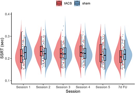
SSRT changes across sessions for the tACS and sham groups. The boxplots show the median and interquartile range to visually summarize central tendency and dispersion. The horizontal line within the box plot represents the median. The top and the bottom lines represent the upper and lower quartiles, respectively. The data points outside of the whiskers are >1.5 quartiles.
Driving performance
Table 2 provides a summary of descriptive and inferential statistics for the braking task. There was no significant interaction between SESSION and TIME for any of the measurements, χ2s < 1.79, ps > 0.18, which suggests that tACS did not impact participants' ability to maintain a safe following distance during this task.
Descriptive and inferential statistics for braking task performance by group and time point. THW is in seconds. Regular refers to performance while following the regularly braking lead vehicle, while irregular refers to performance while following the irregularly braking lead vehicle.
| Mean ± CI | |||||
|---|---|---|---|---|---|
| tACS | Sham | Session × time interaction | |||
| Dependent variable | Session 0 | Session 6 | Session 0 | Session 6 | Chi-square value and P-value |
| Speed variability (km/h) – Irr | 0.37 ± 0.19 | 0.34 ± 0.18 | 0.21 ± 0.07 | 0.33 ± 0.41 | χ2 = 1.79, P = 0.181 |
| Speed variability (km/h) – Reg | 0.23 ± 0.15 | 0.24 ± 0.13 | 0.23 ± 0.07 | 0.19 ± 0.09 | χ2 = 0.66, P = 0.416 |
| THW (s) - Irr | 1.79 ± 0.41 | 1.76 ± 0.43 | 1.38 ± 0.25 | 1.85 ± 1.07 | χ2 = 0.48, P = 0.488 |
| THW (s) - Reg | 1.61 ± 0.33 | 1.50 ± 0.31 | 1.38 ± 0.23 | 1.33 ± 0.17 | χ2 = 0.37, P = 0.545 |
Irr, irregular. Reg, regular.
Table 3 provides a summary of descriptive and inferential statistics for the general driving task.
Descriptive and inferential statistics for the general driving task performance by group and time point.
| Mean ± CI | |||||
|---|---|---|---|---|---|
| tACS | Sham | Session × time interaction | |||
| Dependent variable | Session 0 | Session 6 | Session 0 | Session 6 | Chi-square and P-value |
| Speed variability (km/h) | 2.94 ± 0.37 | 3.45 ± 0.75 | 2.82 ± 0.48 | 2.70 ± 0.43 | χ2 = 1.03, P = 0.309 |
| Median speed (km/h) | 50.64 ± 0.62 | 52.35 ± 1.65 | 50.6 ± 0.70 | 50.53 ± 0.68 | χ2 = 6.32, P = 0.012 |
| Speeding (>5 km/h) | 8.09 ± 4.29 | 20.19 ± 14.41 | 7.15 ± 5.00 | 4.04 ± 3.02 | χ2 = 3.29, P = 0.070 |
| Lane variability (m) | 0.26 ± 0.04 | 0.26 ± 0.04 | 0.25 ± 0.03 | 0.27 ± 0.04 | χ2 = 0.08, P = 0.782 |
| DRT false alarms (N) | 1.00 ± 0.45 | 2.15 ± 1.18 | 1.06 ± 0.63 | 1.58 ± 0.79 | χ2 = 0.54, P = 0.464 |
| DRT hit (%) | 89.72 ± 3.34 | 90.68 ± 1.65 | 91.17 ± 1.86 | 93.32 ± 1.97 | χ2 = 0.128, P = 0.721 |
| Correct DRT RT (ms) | 610 ± 29 | 572 ± 39 | 579 ± 37 | 565 ± 35 | χ2 = 4.91, P = 0.026 |
DRT, detection response task. Bolded values denote statistically significant findings.
There was no significant interaction between SESSION and TIME for lane variability, which suggests that tACS did not affect how well participants maintained a consistent position on the road. There was a significant interaction for median speed. FU contrasts revealed that median speed increased by 1.71 km/h in the tACS group between session 0 and session 6, z = 3.61, P < 0.001, d = 1.37, while the sham group exhibited no significant changes, −0.07 km/h, z = 0.01, P = 0.996, d = 0.002. Importantly, however, there was no corresponding increase in speeding (ie time spent exceeding the limit > 5 km/h) for the tACS group relative to the spam group. There was also no increase in speed variability, suggesting that the tACS group maintained their increased speed consistently.
For the visual DRT, there was a significant interaction between SESSION and TIME on RT, where the tACS group responded faster when detecting targets between session 0 and session 6, −38 ms, z = 3.91, P < 0.001, d = 1.502, while the sham group showed no statistically significant changes, −14 ms, z = 0.69, P = 0.493, d = 0.273. FU contrasts indicated that the baseline differences in DRT response time between the groups were not statistically significant, z = 1.69, P = 0.09, d = 1.03), but neither was the difference between the groups at session 6 (z = 0.29, P = 0.77, d = 0.20). Overall, this suggests that the tACS group improved their response time to DRT stimuli after tACS intervention, indicating improved spare cognitive capacity while driving in session 6 compared to session 0. However, we cannot conclude that the tACS group had more spare capacity at session 6 (post-stimulation) than the sham group. There was no significant interaction between SESSION and TIME for DRT accuracy (Table 2).
Taken together, these results suggest that for the general driving task, the tACS group maintained a faster speed but without a significant increase in excessive speeding (> 5 km/h over the limit) or a corresponding increase in lane position or speed variability, however, with potentially increased spare cognitive capacity.
Discussion
The current study investigated whether repeated applications (ie 5 sessions in 2 wk) of bifocal tACS at beta frequency targeting the rIFG and preSMA, cortical nodes that are thought to play an important role in response inhibition, enhance functional connectivity between these regions and improve response inhibition in healthy young adults. Notably, the focus on repeated applications of tACS in this research represents a novel approach, as most existing studies have examined the effects of tACS in a single session. Furthermore, we explored the potential effect of tACS-induced modulations in the brain on the real-world skill of driving performance, which requires the orchestration of multiple cognitive functions, representing a novel investigation in this field.
The EEG ImCoh measure indicated improved functional connectivity between the rIFG and preSMA following repeated tACS sessions, while no significant effects of tACS on response inhibition or driving braking tasks were observed either within or between sessions. However, for the general driving task, compared to their baseline, participants showed an increased capacity for cognitive load (faster DRT responding), suggesting the potential benefit of bifocal tACS on multiple brain functions despite specifically targeting the response inhibition network. This pattern was absent in the sham group, indicating that the observed effects were specific to the active stimulation. It is important to note that the general driving task primarily reflects fundamental vehicle control, which does not directly engage response inhibition processes. While we observed changes in brain connectivity, these did not correspond to changes in SSRT or targeted braking task performance, suggesting that the observed improvements may reflect more general enhancements in cognitive-motor integration rather than a specific effect on the response inhibition network. Of note, this conjecture is preliminary and should be explored further in future research to establish a more direct link between beta rhythms and cognitive-motor integration. These findings contribute to our understanding of cumulative tACS impacts and their potential real-world applications in complex skills such as driving.
Repeated application of bifocal tACS improves functional connectivity between the rIFG and preSMA over time
In support of our previous studies (Fujiyama et al. 2023), we found no immediate change in rsEEG functional connectivity following bifocal tACS. However, the between-session analysis revealed sustained increases in functional synchrony (ImCoh) between the rIFG and preSMA, consistent with previous evidence of repeated single-site tACS sessions producing enduring effects on connectivity (Khan et al. 2023). Specifically, the tACS group showed significant increases in ImCoh from session 1 to session 5 in our study, which was sustained at the 7-d FU. This is a particularly novel finding, to the best of our knowledge, as it is the first demonstration of significant improvements in functional connectivity following multi-session stimulation using bifocal tACS, specifically targeting connectivity between the 2 cortical regions. Encouragingly, our results provide further evidence that repeated applications of bifocal tACS can lead to significant and long-lasting changes in brain connectivity, particularly within networks associated with cognitive functions.
While we found improved functional connectivity in the active tACS groups, it is important to note that the sham group exhibited a decline in ImCoh across sessions, possibly suggesting the unstable nature of ImCoh from session to session. However, as the tACS group showed the opposite pattern of change, the change in the sham group does not undermine our findings, as it shows that bifocal tACS has a distinct effect on functional connectivity when measured with ImCoh. Given that the current study used in-phase stimulation, i.e. the phase relationship between 2 sinusoidal currents was 0°, future research is warranted to include antiphase (180° phase relationship) stimulation to better delineate the impact of in-phase bifocal tACS on functional connectivity.
There is evidence to suggest that rsEEG offers several advantages over task-related EEG, including its predictive capacity for cognitive performance, stability over time, and ability to capture intrinsic network properties. Beta-2 power (22–29 Hz) at rest has been shown to reliably predict attentional performance, RTs, and frontoparietal network flexibility (Rogala et al. 2020). Unlike task-related EEG, which reflects transient cognitive states, rsEEG provides a stable neural signature of cognitive adaptability, making it particularly valuable in understanding inter-individual variability in response inhibition (Rogala et al. 2020; Buján et al. 2022). Moreover, rsEEG eliminates task compliance issues, making it especially useful in clinical populations, and serves as a scalable, trait-level biomarker across different cognitive conditions (Gu et al. 2022; Afek et al. 2025). While task EEG can offer insights into transient state changes, resting-state connectivity better reflects long-range frontoparietal communication, which is crucial for response inhibition (Rogala et al. 2020). Nevertheless, it is potentially important for future research to consider task-related EEG to further characterize the electrophysiological changes related to the repeated application of bifocal tACS.
Repeated application of bifocal tACS did not improve response inhibition across sessions
Repeated applications of bifocal tACS at 20 Hz (ie beta frequency) over the rIFG and preSMA did not produce significant changes in response inhibition, nor were there improvements observed within sessions. This appeared to contrast with prior findings, which demonstrated that cognitive functions such as working memory (Reinhart and Nguyen 2019) and response inhibition (Fujiyama et al. 2023) can be enhanced by a single session of bifocal tACS. Additionally, repeated applications of unifocal tACS have been shown to result in lasting cognitive improvements (Grover et al. 2022). The absence of significant improvements in response inhibition may reflect differences in the timing of stimulation relative to the task. Our previous study (Fujiyama et al. 2023), which compared the effects of a single session of bifocal tACS applied during versus prior to the SST, found that response inhibition improved but only in the group that received stimulation immediately prior to task performance. In the current study, we applied bifocal tACS during the task, providing further evidence that “online” bifocal tACS does not improve response inhibition when assessed with the SST.
With respect to the between-session changes, while Grover et al. (2022) found that repeated applications of unifocal tACS (4 consecutive days) resulted in lasting cognitive improvements, it is important to note that their study employed a different cohort, ie older adults, while our study focused on healthy young adults. The age difference between the cohorts may have contributed to the differing results. Older adults often exhibit cognitive decline (Hedden and Gabrieli 2004) and might have more room for improving their behavior and may be more responsive to interventions such as bifocal tACS. In contrast, cognitive function in healthy young adults is likely intact, potentially making it more challenging to induce notable modulations in cognitive function within the time frame of a single or repeated tACS session. This could explain why we observed no between-section effects in response inhibition. Additionally, differences in the tasks used could play a role. Response inhibition—as measured by the SST—may require more extended time frames or more stimulations to show changes compared to functions like working memory. These factors—along with potential cohort differences—highlight the complexity of tACS effects across age groups and task types. Further research into the temporal dynamics of stimulation and function-specific responses is crucial to understanding how repeated bifocal tACS improves cognitive functions.
The lack of significant changes in response inhibition while observing modulations in beta oscillations-based connectivity following repeated bifocal tACS may highlight a complex relationship between beta oscillations and response inhibition. Despite significant changes in beta coherence following tACS, we observed no clear behavioral effects, prompting further exploration. Recent work by Errington et al. (2020) challenges the direct link between beta bursts and response inhibition, suggesting that their infrequent occurrence may not directly account for stopping behavior. This raises questions about the functional role of beta oscillations in response inhibition. Our findings suggested that beta rhythms play a nuanced role; beta oscillations might indirectly influence response inhibition by modulating cortical excitability or information flow. Individual variability in the beta-power relationship could also explain inconsistent behavioral effects. Future research is warranted to combine temporal analysis of beta bursts with trial-by-trial behavioral measures and to explore interactions with other frequency bands to better understand the role of beta oscillations in response inhibition.
Repeated application of bifocal tACS may improve general driving performance
We did not observe a significant impact of repeated application of 20 Hz bifocal tACS over the rIFG and preSMA on performance on the targeted driving behavior (braking task), a driving task that involves the ability to adapt behavior and inhibit prepotent responses. This finding suggests that while bifocal beta tACS may influence other aspects of cognitive or motor functions, its effects did not extend to this specific measure of braking task, which involved maintaining a safe distance while following a lead vehicle that braked periodically. In contrast, general driving performance showed some evidence of change after 5 sessions of tACS intervention. Participants in the tACS group drove faster, but without a corresponding increase in speeding or speed variability relative to the sham condition. It is important to note that the observed increase in median speed does not necessarily indicate better adherence to the speed limit, but rather reflects changes in driving behavior after the repeated application of tACS. As such, this suggests that, in line with task instructions, they were able to maintain a stable, faster speed (no increased speeding and no increased lane position and speed variability). Participants in the tACS group also responded faster to the DRT targets after bifocal tACS compared to their baseline, which suggests that tACS increased their spare cognitive capacity (Castro et al. 2019). This suggests that participants in the tACS group potentially had more cognitive resources available during driving after bifocal tACS, which could enhance their ability to manage distractions if they were to occur (ISO 17488, 2016).
Our results align with Facchin et al. (2023), who observed improved attentional capacity, measured by a DRT following 3 sessions of transcranial direct current stimulation, another form of tES (tDCS), targeting the frontal eye field, a region implicated in target selection and distractor suppression (eg Corbetta and Shulman 2002). Similarly, previous tDCS studies targeting the dorsolateral prefrontal cortex (DLPFC) have shown positive effects on driving. Sakai et al. (2014) found that tDCS with an anodal electrode over the right DLPFC enhanced car-following and lane-keeping behavior, while Beeli et al. (2008) demonstrated that tDCS with an anodal electrode over the left and right DLPFC reduced risky driving behavior, but did not impact participants’ ability to maintain a safe distance when following a periodically braking lead vehicle.
In the current study, targeting the rIFG and preSMA with bifocal tACS demonstrated a distinct mechanism for improving general driving performance. Unlike prior tDCS studies focusing on the DLPFC and FEF, bifocal tACS applied to regions (rIFG and preSMA) that are implicated in inhibitory function resulted in increased driving speed and improved RT on a DRT, reflecting greater spare capacity. While these driving measures do not specifically assess response inhibition, the results suggest potential broader effects of tACS on cognitive and motor functions relevant to driving performance.
Taken all together, previous findings and our current results highlight the importance of exploring how stimulation of specific brain regions can improve particular functions, which would offer a foundation for tailoring interventions to target distinct cognitive and behavioral outcomes.
Limitations and future perspectives
The present study found that functional connectivity between key regions implicated in response inhibition improved across sessions, while the behavioral manifestation of response inhibition showed no changes following bifocal tACS. The lack of significant changes in response inhibition may raise questions about the efficacy of the bifocal tACS protocol used. Individual response variability to tACS may account for this discrepancy, indicating that a one-size-fits-all approach may not be optimal for all participants. Although the tACS protocol was based on established brain oscillations linked to response inhibition (Swann et al. 2011; Aron et al. 2016), individual variability in brain oscillations could affect its effectiveness. Tailoring tACS frequencies to match participants' unique peak oscillations might optimize performance (Vosskuhl et al. 2015; Veniero et al. 2019) or utilizing a closed-loop approach to optimize stimulation parameters during the stimulation by monitoring neurophysiological readouts (Wansbrough et al. 2024) would potentially reduce individual variability. Furthermore, greater spare cognitive capacity has been related to improved driver safety and better hazard response (Strayer et al. 2015), and shown to quantify the workload induced by in-car technology distractions (Strayer et al. 2017; Bowden et al. 2019).
Our study had sufficient statistical power to detect EEG changes pre- and post-stimulation. However, future research should increase participant numbers to better investigate correlations between changes in brain connectivity and behavioral improvements. Exploratory analyses of the correlations between ImCoh ratio changes and improvements in SSRT, driving, and braking performance revealed medium effect sizes (Kendall’s Tau range: −0.6 to +0.4), but these were not statistically significant (ps > 0.21), and Bayesian statistics yielded anecdotal evidence (BF10s < 2.15) (Wagenmakers et al. 2018). While these findings do not establish a relationship between functional connectivity modulation and behavioral improvements, they also do not definitively rule one out. Future studies should further explore potential associations between functional connectivity changes and behavioral outcomes, particularly in the context of repeated bifocal tACS applications.
Similarly, individual differences in response to NiBS are crucial to consider (eg Hamada et al. 2012). Future work should prioritize person-specific neural dynamics to uncover hidden response patterns. This can be achieved by incorporating time-varying connectivity analysis, which has been shown to reveal dynamic shifts in functional brain states and their relationship to cognitive processes (Kucyi 2018). Additionally, individualized computational modeling may help identify subgroups of "best responders" with unique neuro-behavioral profiles by tailoring models to individual variability in brain network dynamics (Finn et al. 2015). Furthermore, adopting a closed-loop approach, as suggested by Wansbrough et al. (2024), could offer real-time neuromodulation by dynamically adjusting interventions based on ongoing brain activity. This technique would enable precise modulation of spontaneous brain states, fostering a deeper understanding of the interaction between transient neural dynamics and cognitive interventions. By integrating these advanced methodologies with multimodal imaging (eg EEG-fMRI) and longitudinal behavioral tracking, future studies can bridge population-level findings with personalized mechanisms, ultimately informing tailored strategies for optimizing brain plasticity and cognitive enhancement.
Additionally, the timing of the sessions, ie 5 stimulation sessions over 14 d, may have influenced the outcomes. While our protocol closely aligns with that of Antonenko et al. (Antonenko et al. 2023), Grover et al. (2022) applied unifocal tACS targeting the DLPFC and inferior parietal lobule over 4 consecutive days and observed significant, long-lasting improvements in working memory performance in older adults. This suggests that a more condensed stimulation schedule may be a key factor in driving cognitive benefits, warranting further investigation into the optimal timing and frequency of tACS interventions.
Conclusion
The present study was the first to investigate repeated sessions of bifocal tACS over the rIFG and preSMA for improving response inhibition, functional connectivity, and driving performance. Significant improvements in functional connectivity and, potentially, in general, driving performance were observed, highlighting the potential of tACS to modulate connectivity and enhance driving performance over time. While changes in response inhibition were not detected, the extended effects on functional connectivity suggest the possibility of long-term benefits for conditions related to cortical connectivity. The lack of notable changes in response inhibition may be attributed to individual differences and parameter thresholds, as well as differences between “online” and “offline” effects of tACS. Despite this, the findings provide novel insight into the use of bifocal tACS for neuromodulation, offering a foundation for further exploration of bifocal tACS to enhance functional connectivity and associated cognitive and motor processing.
Acknowledgments
The authors thank Ms Arabella Graham, Ms Tianah Linnell, Ms Alana Vincent, and Ms Paige Morgan for their contribution to the data collection.
Author contributions
Hakuei Fujiyama (Conceptualization, Formal analysis, Funding acquisition, Investigation, Methodology, Project administration, Resources, Software, Supervision, Validation, Visualization, Writing—original draft, Writing—review & editing), Vanessa Bowden (Conceptualization, Formal analysis, Methodology, Writing—review & editing), Alexander Tang (Conceptualization, Formal analysis, Methodology, Writing—review & editing), Jane Tan (Conceptualization, Investigation, Methodology, Writing—review & editing), Elisha Librizzi (Investigation, Writing—review & editing), and Shayne Loft (Conceptualization, Methodology, Writing—review & editing).
Funding
This work was supported by the Neurotrauma Research Program (DoH20193370) awarded to H.F., J.T., V.B., A.T., and S.L. A.D.T was supported by a Sarich Family Research Fellowship.
Conflict of interest statement
The authors declare that they have no known financial, professional, or personal conflicts of interest that could have influenced the work reported in this [manuscript/study/proposal]. No funding bodies had any role in the study design, data collection, analysis, interpretation, or decision to submit this work for publication.