


Abstract
Single-cell Hi-C data are a common data source for studying the differences in the three-dimensional structure of cell chromosomes. The development of single-cell Hi-C technology makes it possible to obtain batches of single-cell Hi-C data. How to quickly and effectively discriminate cell types has become one hot research field. However, the existing computational methods to predict cell types based on Hi-C data are found to be low in accuracy. Therefore, we propose a high accuracy cell classification algorithm, called scHiCStackL, based on single-cell Hi-C data. In our work, we first improve the existing data preprocessing method for single-cell Hi-C data, which allows the generated cell embedding better to represent cells. Then, we construct a two-layer stacking ensemble model for classifying cells. Experimental results show that the cell embedding generated by our data preprocessing method increases by 0.23, 1.22, 1.46 and 1.61|$\%$| comparing with the cell embedding generated by the previously published method scHiCluster, in terms of the Acc, MCC, F1 and Precision confidence intervals, respectively, on the task of classifying human cells in the ML1 and ML3 datasets. When using the two-layer stacking ensemble framework with the cell embedding, scHiCStackL improves by 13.33, 19, 19.27 and 14.5 over the scHiCluster, in terms of the Acc, ARI, NMI and F1 confidence intervals, respectively. In summary, scHiCStackL achieves superior performance in predicting cell types using the single-cell Hi-C data. The webserver and source code of scHiCStackL are freely available at http://hww.sdu.edu.cn:8002/scHiCStackL/ and https://github.com/HaoWuLab-Bioinformatics/scHiCStackL, respectively.
Introduction
High-throughput chromosome conformation capture (Hi-C) is a technology that uses high-throughput DNA sequencing technology and chromosome conformation capture technology to capture genome-wide chromatin interaction information [1]. The birth of Hi-C technology allows researchers to further analyze the relationship between the three-dimensional structure of the genome and the basic functions of cells [2–5]. However, because of cell type heterogeneity [6–10], traditional bulk Hi-C data have limitations in studying heterogeneous cell populations. Thus, Nagano et al. [11] proposed a single-cell Hi-C technology that can detect chromatin interactions in a single cell.
Initially, researchers tried to apply the computational methods of bulk Hi-C data to single-cell Hi-C data when analyzing the differences in the three-dimensional structures of chromosomes in heterogeneous cell populations [12–15]. Because of the low throughput limitation of original single-cell Hi-C technology [16], the methods for automatically identifying cell types based on single-cell Hi-C data have not been developed. The sciHi-C protocol proposed by Ramani et al. [16] successfully improves the throughput of capturing single-cell chromosome interaction information, which made it possible to classify a large number of heterogeneous cell populations based on single-cell Hi-C data. There are different types of cells when sequencing single-cell Hi-C data of cell populations at the same time. The specificities in heterogeneous cells may be masked if each cell cannot be accurately identified in the experiment. Thus, it is important to classify cells based on single-cell Hi-C data accurately. However, biological methods to detect cell types consume a lot of experimental costs. Thus, it is necessary to use computational methods to identify cell types based on single-cell Hi-C data. Moreover, the single-cell Hi-C data measured in batches are sparse, which is also a challenge for accurately classifying cells based on single-cell Hi-C data. The existing algorithms for classifying heterogeneous cell populations based on single-cell Hi-C data have the following limitations. Firstly, some researchers focus on the classification of different cell cycles [17–19]. However, the performance of these algorithms in predicting unidentifed cell types at the same cell stage is still unknown. Secondly, Zhou et al. [20] proposed a clustering algorithm (scHiCluster) to predict unidentified cell types based on single-cell Hi-C data. scHiCluster used a convolution smoothing algorithm and a random walk with restart algorithm to process the chromosome contact matrix in single cell, and used two principal component analyses (PCA) operations to generate cell embeddings. Finally, the scHiCluster used the K-means algorithm to cluster cells based on cell embedding. The scHiCluster algorithm solved preliminarily the problem of how to predict unidentified cell types. However, high-precision classification algorithms are still limited in terms of classifying the identified cells.
In this study, we propose a computational framework to achieve high-precision cell classification based on sparse single-cell Hi-C data. We propose a novel cell embedding- and stacking ensemble learning-based approach, called scHiCStackL, to classify heterogeneous cell groups based on single-cell Hi-C data. We first improve the data preprocessing part of the scHiCluster algorithm by using the following steps. (1) Based on the characteristics of the three-dimensional structure of the chromosome, we use the close contact information in the space to smooth the chromosome contact matrix to solve the sparsity of the contact matrix. (2) We use Kernel principal component analysis (KPCA) to generate cell embedding to retain more contact feature information. Then, we construct a stacking ensemble model to classify cells based on three traditional classification algorithms. Finally, we conduct a comprehensive comparison of the scHiCStackL and previously published algorithms. The analysis shows that our proposed scHiCStackL framework can significantly improve the classification performance in predicting cell types based on sparse single-cell Hi-C data.
Materials and methods
Datasets
The dataset we used is the low coverage dataset downloaded from the GEO database: namely, Ramani dataset and Flyamer dataset [16, 18]. We mainly focus on two parts of the Ramani dataset: ML1 and ML3. The interaction pairs and cell quality files of ML1 and ML3 are all downloaded from GSE84920. ML1 and ML3 contain four human cells (HeLa, HAP1, GM12878 and K562) and two mouse cells (MEF1 and Patski). In the dataset file, the cell quality file contains specific information of the cell, such as the cell type, the percentage of the captured fragments mapped to the mouse and human whole gene sequences, etc. The interaction pairs file contains specific information about the contact of chromosome fragments in the cell, such as the start position of the contact fragment and the end position of the contact fragment. In addition, the number of contacts captured by cells in the dataset we used mainly ranges from 5.2K to 35K. The interaction files of Flyamer dataset are all downloaded from GSE80006 [18]. For the Flyamer dataset, we select contact files with a resolution = 200K. The Flyamer dataset includes three types of mouse cells: Oocyte (NSN and SN), ZygP and ZygM. The number of contacts in the Flyamer dataset ranges from 1.4K to 1.65M. Since our algorithm mainly deals with sparse single-cell Hi-C data, we randomly downsample so that the number of contacts of each cell in the Flyamer dataset ranges from 1.4 to 35K.
Data preparation
Because of some irrevelant data in the dataset, it is necessary to ensure the quality of the research data. As our research mainly focuses on cell classification in the four human cell lines, we firstly screen out the cells that are not from humans in the Ramani dataset [16]. Then, we screen out these simulated cells as Ramani et al. generated a lot of irrelevant simulated cell data. To prevent some cells with a minimal number of read-pairs from affecting the final clustering and classification results, we set a contact threshold |$th_{1}=5K$|, which is used to screen out cells with a total contact number less than 5K.
Framework of scHiCStackL
We illustrate the cell embedding- and stacking ensemble learning-based framework of scHiCStackL in Figure 1 [22, 23]. There are two crucial steps in the scHiCStackL framework: cell embedding generation and stacking ensemble learning. In this section, we describe the two-step workflows of the scHiCStackL framework step by step.
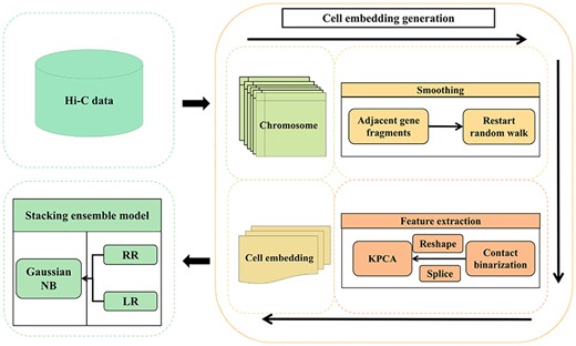
The overall framework of scHiCStackL.
Cell embedding generation
Stacking ensemble learning
In this step, we construct a stacking ensemble model to classify cells based on the cell embedding generated in the previous step [22, 23], where the cell embedding is used as the feature vector of the cell. Since the feature vector generated by the KPCA dimensionality reduction algorithm is linear, the base classifiers we choose are classifiers based on linear models: ridge regression (RR) classifier [23, 30] and logistic regression (LR) classifier [31, 32]. And the meta-classifier in the second layer is a Gaussian naive bayes (GaussianNB) [33, 34]. The structure of the Stacking ensemble model we constructed is shown in Figure 2.
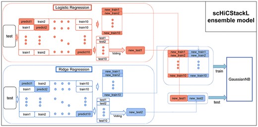
The structure of the scHiCStackL ensemble model.
1. To avoid the problem of model overfitting [35], we use a 10-fold cross-validation algorithm and random sampling algorithm to divide the training dataset |$S_{D}$| into 10 parts: |$S_{1}, S_{2},..., $|and |$S_{10}$| [36, 37]. For the |$k$|th |$(k=1, 2,..., 10)$| training, we choose |$S_{D}-S^{k}_{D}$| and |$S^{k}_{D}$| as the current training dataset and test dataset, respectively. |$S^{k}_{D}$| is used to generate a new training dataset based on the predicted value of the base classifier. Thus, the training dataset generated in the |$k$|th iteration is |$S^{k}_{D\_new}=\{(\Omega ^{k}_{l}(x_{j}), y_{j})\}((x_{j}, y_{j})\in ^{k}_{D}, l=1, 2)$|. Then, the training dataset |$S_{T}$| is transformed into a new dataset |$S^{k}_{T\_new}=\{\Omega ^{k}_{l}(x_{j})\} (x_{j}\in S_{T}, l=1, 2)$| based on the prediction of the base classifier in the |$k$|th iteration.
2. We integrate 10 new training datasets into a new training dataset |$S_{D\_new}=\{(S^{k}_{D\_new}), k=1, 2,..., 10\}$|, which serves as the second-level training dataset. Since our data have multiple class labels, we use voting to generate the test dataset |$S_{T\_new}=\{Mode(\Omega ^{k}_{l}(x_{j})), x_{j}\in S_{T}, k=1, 2,..., 10, l=1, 2\}$| of the second layer (Mode() is a function to find the mode).
In the next step, the new training dataset |$S_{T\_new}$| is used to train the GaussianNB classifier in the second layer. The new test dataset is used to evaluate the performance of the stacking ensemble model we built. In addition, it is worth noting that we use the 5-fold cross-validation strategy and random sampling algorithm to divide the training set and test set to prevent the model overfitting.
Results
In this section, we compare scHiCStackL with multiple algorithms to evaluate its performance in classifying sparse singel-cell Hi-C data. [20]. In order to facilitate comparison, we use accuracy (Acc), Matthew’s correlation coefficient (MCC), F1-score (F1) and Precision to evaluate the classification results [38–40], and use adjusted Rand index (ARI), normalized mutual information (NMI) and adjusted mutual information (AMI) to evaluate the clustering results [41–44]. In addition, we use the bootstrap method to calculate the confidence interval of the multi-dimensional clustering and classification results for the sake of analyzing the comparison results.
Performance evaluation of cell embedding generation method
Since our cell embedding generation method is an improvement of the scHiCluster method [20], we first compare the data preprocessing part of the scHiCStackL method with that of scHiCluster. We use two cell embedding generation methods to process the dataset (including 626 human cells after data preparation in ML1 and ML3) to generate two cell embeddings: scHiCStackL cell-embedding and scHiCluster cell-embedding [16, 20]. We use the grid optimization algorithm to obtain the parameters in the cell embedding generation method. After experimental testing, we use linear kernel as kernel function of KPCA. In order to compare the effects of the two cell embedding generation methods, we use the K-means method to cluster the two cell embeddings with reference to the clustering part of the scHiCluster method. We select a certain number of principal components as the features of the cell. As shown in Supplementary Figure S1, the most experimental results are unstable when the fore 10-dimensional principal components are used as features. Thus, we choose the comparison of results starting from the fore 11-dimensional principal components. When the cell features are the fore 11–20 dimensional principal components, the clustering results of the two cell embeddings tend to be stable. Thus, in order to compare the clustering performance of the two cell embeddings, we use the bootstrap method to calculate the confidence interval of the clustering results from the fore 11–20 dimensional principal components. The comparison of the clustering results of the two cell embeddings is shown in Figure 3 (|$99\%$| confidence interval comparison) and Supplementary Figure S2 (comparison of the results of the principal components of each dimension).
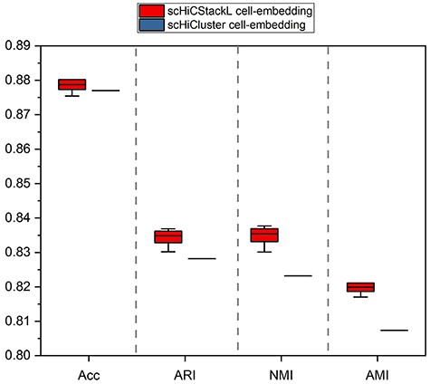
Comparison of the clustering effect of the two cell embeddings on ML1 and ML3 datasets. The upper and lower edges indicate the maximum and minimum values of the results, respectively. The box represents the confidence interval of the results. (The confidence interval of scHiCluster cell-embedding is shown as a line in the figure due to the smaller confidence interval.).

The classification effect comparison of different combinations of the improved sub-steps (Adj and KPCA) and the original sub-steps (Con and two PCA). The upper and lower edges indicate the maximum and minimum values of the results, respectively. The box represents the confidence interval of the results.
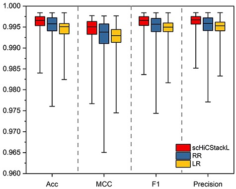
The comparison between scHiCStackL and the base classifier is based on the |$99\%$| confidence interval of results. The upper and lower edges indicate the maximum and minimum values of the results, respectively. The box represents the confidence interval of the results.
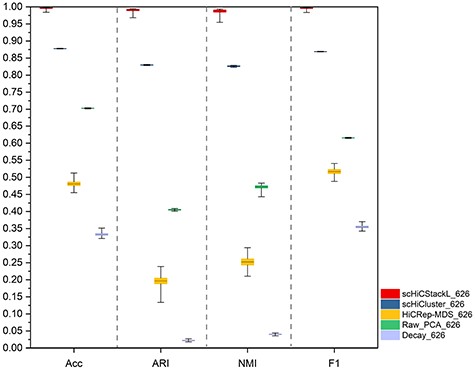
The comparison between scHiCStackL and four methods (scHiCluster, HiCRep-MDS, Raw_PCA and Decay) is based on the |$99\%$| confidence interval of results(ML1 and ML3 datasets). The five methods are scHiCStackL, scHiCluster, HiCRep-MDS, Raw_PCA and Decay from left to right. The upper and lower edges indicate the maximum and minimum values of the results, respectively. The box represents the confidence interval of the results.
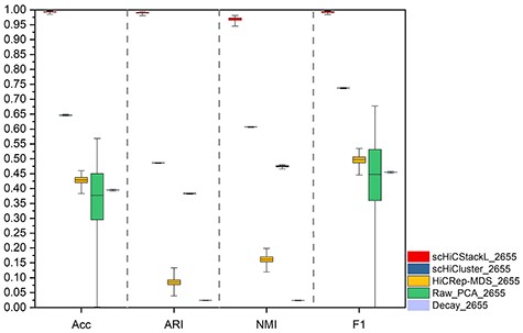
The comparison between scHiCStackL and four methods (scHiCluster, HiCRep-MDS, Raw_PCA and Decay) is based on the |$99\%$| confidence interval of results(the whole Ramani dataset). The five methods are scHiCStackL, scHiCluster, HiCRep-MDS, Raw_PCA and Decay from left to right. The upper and lower edges indicate the maximum and minimum values of the results, respectively. The box represents the confidence interval of the results.
From the results provided in Figure 3 and Supplementary Figure S2, we conclude that scHiCStackL cell-embedding achieves a better clustering result in comparison with scHiCluster cell-embedding in terms of Acc ([0.877, 0.877] versus [0.877, 0.88]), ARI ([0.828, 0.828] versus [0.833,0.836]), NMI ([0.823,0.823] versus [0.833, 0.837]), and AMI ([0.807, 0.807] versus [0.819, 0.821]). Moreover, we also compare the clustering results of the two data preprocessing methods on the downsampled Flyamer dataset [18]. The comparison results of the two embedding generation methods on the downsampled Flyamer dataset are shown in Supplementary Figure S3 (|$99\%$| confidence interval comparison) and Supplementary Figure S4 (comparison of the results of the principal components of each dimension) [18]. Supplementary Figures S3 and S4 demonstrate that scHiCStackL cell-embedding outperforms scHiCluster cell-embedding in terms of Acc, ARI, NMI and AMI on the downsampled Flyamer dataset. These results show that our improved cell embedding can better represent the three-dimensional structure of the chromosome in the cell.
Moreover, we compare the classification effects of the cell embedding generated by the combination of the original substeps (Con and Twice PCA) and the improved substeps (smoothing of adjacent gene fragments (Adj) and KPCA) in the Stacking ensemble model to prove that scHiCStackL cell-embedding is more suitable for the stacking ensemble model we constructed. Here, we use MCC, Acc, F1 and Precision to evaluate the final classification results. When the fore 11–50 dimensional principal components are used as cell characteristics, the comparison results are shown in Figure 4 (|$99\%$| confidence interval comparison) and Supplementary Figure S5 (comparison of the results of the principal components of each dimension).
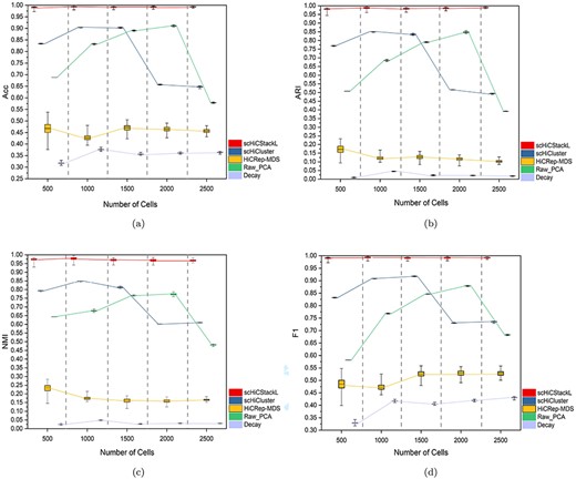
The comparison between scHiCStackL and four methods (scHiCluster, HiCRep-MDS, Raw_PCA and Decay) on five different scale (500, 1000, 1500, 2000, 2500) datasets. The performances of five methods are compared using the Acc(a), ARI(b), NMI(c) and F1(d) evaluation indicators. The five methods are scHiCStackL, scHiCluster, HiCRep-MDS, Raw_PCA and Decay from left to right. The upper and lower edges indicate the maximum and minimum values of the results, respectively. The box represents the confidence interval of the results.
In the ensemble model of scHiCStackL, the cell embedding generated by our improved method achieves the optimal Acc confidence interval of [0.995, 0.997], MCC confidence interval of [0.993, 0.996], F1 confidence interval of [0.995, 0.997] and Precision confidence interval of [0.996, 0.998], respectively. Although the original cell embedding only reaches the Acc confidence interval of [0.988, 0.99], MCC confidence interval of [0.983, 0.985], F1 confidence interval of [0.988, 0.99] and Precision confidence interval is [0.989, 0.991]. The results show our improved substeps are suitable for combining with the stacking ensemble model we established to classify the four types of cells from the Ramani dataset.
Classification performance evaluation of ensemble model in scHiCStackL
Next, we evaluate the classification performance of the established stacking ensemble model and compare the results with two base classifiers (LR and RR). The cell embedding applied to the established stacking ensemble model and the two base classifiers are all generated by our improved method. After testing, we choose KPCA with the sigmoid kernel function to generate the final cell embedding. Similarly, we use MCC, Acc, F1 and Precision to evaluate the final classification results. The evaluation of the classification results is shown in Figure 5 (|$99\%$| confidence interval comparison) and Supplementary Figure S6 (comparison of the results of the principal components of each dimension).
Figure 5 and Supplementary Figure S6 demonstrate that scHiCStackL achieves optimal performance in terms of Acc confidence interval [0.995, 0.997], MCC confidence interval [0.993, 0.996], F1 confidence interval [0.995, 0.997] and Precision confidence interval [0.996, 0.998]. Although RR and LR reaches the Acc confidence interval of ([0.994, 0.997] and [0.993, 0.996]), MCC confidence interval of ([0.991, 0.996] and [0.991, 0.994]), F1 confidence interval ([0.994, 0.997] and [0.994, 0.996]), and Precision confidence interval ([0.994, 0.997] and [0.994, 0.996]). These results show that scHiCStackL integrates the base classifier and achieves better and more stable performance.
Evaluation of scHiCStackL’s performance in predicting cell types
In this section, we compare scHiCStackL with scHiCluster, HiCRep-MDS, Raw_PCA and Decay methods on the ML1 and ML3 datasets, Ramani dataset and Flyamer dataset [16–18, 45]. Kmeans clustering algorithm is utilized to cluster the embeddings generated by HiCRep-MDS, Raw_PCA and Decay on ML1 and ML3 datasets, which contains 626 human cells after data preparation. Here, we use Acc, ARI, NMI and F1 evaluation indicators to evaluate the performance of the five methods. The results are shown in Supplementary Table S4 (confidence interval of the results of each method), Figure 6 (confidence interval comparison) and Supplementary Figure S7 (comparison of the classification results of each dimension).
From the results provided in Supplementary Table S4, Figure 6 and Supplementary Figure S7, the experimental results achieved by the HiCRep-MDS, Decay and Raw_PCA methods are poor on the ML1 and ML3 datasets. However, scHiCluster and scHiCStackL achieve better performance in terms of Acc confidence interval ([0.878, 0.878] versus [0.995, 0.997]), ARI ([0.829, 0.830] versus [0.989, 0.992]), NMI ([0.825, 0.827] versus [0.984, 0.990]) and F1 ([0.869, 0.869] versus [0.995, 0.997]).
Then, we select the whole Ramani dataset, which contains 2655 human cells after data preparation, to evaluate the performance of scHiCStacL, scHiCluster, HiCRep-MDS, Raw_PCA and Decay methods. The comparison results are shown in Supplementary Table S4, Figure 7 and Supplementary Figure S8 (comparison of the classification results of each dimension).
Figure 7 and Supplementary Figure S8 show that scHiCStackL still has superior performance comparing to the other four methods on the whole Ramani dataset. Moreover, we also compare the performance of the five methods on the Flyamer dataset. The comparison results are shown in Supplementary Table S4, Supplementary Figures S9 and S10, which demonstrate that scHiCStackL achieves better performance compared with scHiCluster, HiCRep-MDS, Raw_PCA and Decay methods on the Flyamer dataset. All these results indicate that our proposed scHiCStackL method achieves optimal performance in predicting cell types.
In order to prove the robustness of scHiCStackL when processing datasets of different sizes, we compare the performance of scHiCStackL, scHiCluster, HiCRep-MDS, Raw_PCA and Decay methods on 5 different scale datasets by randomly selecting 500, 1000, 1500, 2000 and 2500 cells from the Ramani dataset. Then we conduct analysis on the results of scHiCStackL, scHiCluster, HiCRep-MDS, Raw_PCA and Decay methods based on these datasets, which are shown in Supplementary Table S5, Figure 8 and Supplementary Figures S11–S15.
Supplementary Table S5 shows that the clustering results achieved by the HiCRep-MDS and Decay method are poor on five different scale datasets. Figure 8 and Supplementary Figures S11–S15 show scHiCStackL, on different scale datasets, maintains better performance than scHiCluster and Raw_PCA in terms of confidence interval for Acc, ARI, NMI and F1. Moreover, these results also prove that our algorithm has strong robustness on datasets of different scales.
Discussions and limitations
In this study, we first improve Zhou et al.’s cell embedding generation method by interpolating more chromosome structure information and retaining more chromosome structure features. In the stacking ensemble model, we choose the linear classifiers as the base classifiers, which is easier to fit the data generated by KPCA dimensionality reduction. The stacking ensemble model combines the advantages of the two base classifiers through voting methods. Moreover, the model better fits the cell embedding through training, and achieves high-precision cell classification. We compare our improved cell embedding generation method with the original cell embedding generation method in scHiCluster [20]. Compared with the original cell embedding generation method, the cell embedding generation method in scHiCStackL achieves competitive performance on the four evaluation indicators. In addition, we compare the performance of scHiCStackL, scHiCluster, HiCRep-MDS, Raw_PCA and Decay in predicting cell types on the Ramani dataset and Flyamer dataset. On Ramani and Flyamer datasets, scHiCStackL has far better performance than other four methods in terms of four evaluation indicators. These results demonstrate that scHiCStackL has a good ability in classifying cells and strong robustness. However, there are few high-throughput sparse single-cell Hi-C data at present. As more and more sparse single-cell Hi-C data are obtained in the future, the practicality of scHiCStackL is expected to be further improved.
Conclusion
In this study, we propose a novel stacking ensemble learning-based approach for classifying sparse single-cell Hi-C data, called scHiCStackL. The first part of scHiCStackL is an improved version of the existing data preprocessing method for generating cell embedding, and the second part is the stacking ensemble model we established for classifying cells. We first evaluate the performance of the improved data preprocessing method and the original data preprocessing method in terms of clustering and cell classification. The results show that our improved data preprocessing method can better improve the cell classification and clustering performance. Then, we evaluate the performance of the scHiCStackL, scHiCluster, HiCRep-MDS, Raw_PCA and Decay methods in predicting cell types based on sparse single-cell Hi-C data. The results show that our proposed scHiCStackL method has optimal performance comparing to scHiCluster, HiCRep-MDS, Raw_PCA and Decay. In addition, it was found that the continuous cycle stages of cells can be separated based on single-cell Hi-C data [17, 19]. It is hoped that our improved data preprocessing method can be applied to single-cell Hi-C data with cells of different cycles to study the classification of cell cycles in future work.
We propose a novel computational framework, called scHiCStackL, to achieve the high-precision cell classification based on sparse single-cell Hi-C data.
We improve the cell embedding generation method for single-cell Hi-C data proposed by Zhou et al. to improve the ability of cell embedding.
We establish a two-layer Stacking ensemble learning model to achieve high-accuracy cell classification based on cell embedding.
Comprehensive comparison experiments show that the performance of scHiCStackL is far better than that of Zhou et al.’s scHiCluster algorithm in predicting cell types on different scale datasets.
Author contributions statement
Hao Wu, Bing Zhou and Yingfu Wu conceived the experiments. Hao Wu, Yuhong Jiang and Yingfu Wu conducted the experiments. Yingfu Wu, Zhongli Chen and Yuhong Jiang analyzed the results. Yingfu Wu and Haoru Zhou wrote the manuscript. Hongming Zhang, Hao Wu, Yi Xiong and Quanzhong Liu reviewed the manuscript.
Acknowledgments
We thank Biting Liang for their helpful advice and discussions. The work was supported by the National Natural Science Foundation of China (Grant No. 61972322), by the Natural Science Foundation of Shaanxi Province (Grant No. 2021JM-110), by the Humanities and Social Science Fund of the Ministry of Education of China (Grant No.18YJCZH190) and by ‘The Fundamental Research Funds of Shandong University’. The funders did not play any role in the design of the study, the collection, analysis, and interpretation of data, or the writing of the manuscript.
Hao Wu received the BSc and MSc degree in Computer Sciences from Computer College at Inner Mongolia University, and the PhD degree from the School of Computer Science and Technology from Xidian University. He was a visiting scholar at the Knowledge Engineering and Discovery Research Institute, Auckland University of Technology from July 2014 to August 2015. He is currently an associate professor in the School of Software, Shandong University. He has published over 30 works in professional journals and conferences. His research has been funded by NSFC, NSFSP and others. His main research interests include data mining and bioinformatics. He has also served for various journals as reviewer or guest editor.
Hong-Ming Zhang, PhD, is professor. His main research interests are in spatial big data analysis, precision agriculture and bioinformatics..
Ying-Fu Wu is MS candidate. His main research interests are in computational bioinformatics and biological big data mining.
Yu-Hong Jiang is BS candidate. His main research interests are in computational bioinformatics and biological big data mining.
Bing Zhou is MS candidate. His main research interests are in computational bioinformatics and biological big data mining.
Hao-Ru Zhou is MS candidate. Her main research interests are in computational bioinformatics and biological big data mining.
Zhong-Li Chen is MS candidate. His main research interests are in computational bioinformatics and biological big data mining.
Yi Xiong, PhD, is associate professor. His main research interests are protein function prediction and drug discovery and development.
Quan-Zhong Liu, PhD, is associate professor. His main research interests are in bioinformatics and data mining.
References
Author notes
Y. Wu and H. Wu contributed equally to this work.
