


Abstract
Drug resistance is one of the most intractable issues for successful treatment in current clinical practice. Although many mutations contributing to drug resistance have been identified, the relationship between the mutations and the related pharmacological profile of drug candidates has yet to be fully elucidated, which is valuable both for the molecular dissection of drug resistance mechanisms and for suggestion of promising treatment strategies to counter resistant. Hence, effective prediction approach for estimating the sensitivity of mutations to agents is a new opportunity that counters drug resistance and creates a high interest in pharmaceutical research. However, this task is always hampered by limited known resistance training samples and accurately estimation of binding affinity. Upon this challenge, we successfully developed Auto In Silico Macromolecular Mutation Scanning (AIMMS), a web server for computer-aided de novo drug resistance prediction for any ligand–protein systems. AIMMS can qualitatively estimate the free energy consequences of any mutations through a fast mutagenesis scanning calculation based on a single molecular dynamics trajectory, which is differentiated with other web services by a statistical learning system. AIMMS suite is available at http://chemyang.ccnu.edu.cn/ccb/server/AIMMS/.
Introduction
Drug resistance is an important cause of the frequently inevitable failure of targeted drug therapeutics in clinical practice, particularly for the treatment of infectious diseases and cancer [1–5]. Mutation in drug-targeting proteins is one of the primary causes of resistance [6–10]. To better understand and to prevent drug resistance, more and more attentions have been paid to exploring the relationship between the mutations and the related pharmacological profile of drug candidates [11–14], which can advance our knowledge of resistance mechanism and lead to new strategies to treat therapeutic failure [15]. Hence, effective prediction approach estimating the sensitivity of mutations to agents is a new opportunity that counters drug resistance and creates a high interest in pharmaceutical research.
However, traditional hypothesis-driven experimental approaches are time-consuming and expensive because of the necessity for multiple experimental conditions, cell lines and time points. In addition, so far most computational methods are data-driven, which focus on a specific target protein (for example, HIVdb: http://sierra2.stanford.edu/sierra/servlet/JSierra) [16–19]. A sufficient set of resistance and non-resistance samples will be used to train a statistical learning system, which is hard to perform de novo prediction of drug sensitivity to mutations with limited or no training data sets. Therefore, there is an urgent need to develop computational prediction approaches to universally and quantitatively investigate drug response and protein mutation, which can advance our understanding of the underlying mechanisms of drug resistance and facilitate the design of more effective treatment strategies to improve drug efficacy. In addition, de novo method of drug resistance prediction can develop repurposing therapy for existing resistant drug, which is promising to explore alternative ways to counter resistant. However, there is not an online platform for de novo drug resistance prediction up to now.
We have developed a computational mutation scanning (CMS) protocol in previous studies, which can reasonably combine molecular dynamics (MD) simulation and one-step free energy perturbation to quantitatively predict resistances to any drug [15, 20–23]. The operation is based on a single MD simulation of a reference protein–ligand complex and the post-processing of the trajectory, in which each snapshot of the reference is replaced by the mutated residue and using endpoint free energy calculation for an estimation of the contribution of mutation. There are two reasons that this mutation-scanning mode is able to reproduce relative binding free energies at a much lower computational cost compared with the conventional free energy perturbation calculation. First, one-step perturbation does not need to sample a set of intermediate points in the transformation between the states A and B, but provides a more efficient approach for calculating binding free energies based on conformational sampling of just the endpoint. Second, a set of N mutants can be ranked by performing N fast binding free energy analysis instead of the pairwise comparison of N time-consuming MD simulation. Hence, this approach is clearly to be most useful for mutation-induced drug resistance prediction, as was the purpose of this work. Based on CMS, we developed a de novo drug resistance prediction server—Auto In Silico Macromolecular Mutation Scanning (AIMMS). It can be used to scan mutations for protein targets and to predict ratios and mechanism of resistance. The relationship between mutations and the related pharmacological profile of drugs is analyzed to elucidate the contribution of the fixed mutations to the drug resistance. Furthermore, AIMMS was successfully used to predict resistance for HIV-1 protease, HIV reverse transcriptase, influenza virus neuraminidase, kinase, etc., which correlates very well with the corresponding experimental data. This web server is free and open to all users at http://chemyang.ccnu.edu.cn/ccb/server/AIMMS/.
Materials and methods
MD simulation
The complex 3D structure can be obtained from a dock result or directly downloaded from the Research Collaboratory for Structural Bioinformatics (RCSB) protein data bank (PDB; http://www.rcsb.org/pdb/home/home.do) [24]. The AM1-BCC charge model in Antechamber module of Amber16 program was used to assign charges for ligand atoms [25–27]. The topology and coordinate files of the complex were built with the Leap module in Amber16 program. The AMBER ff14SB force field was used for amino acid residues, and general AMBER force field (GAFF) was used for ligands [28–30]. Cl- or Na+ was added to neutralize the system. All the molecules were solvated in a rectangular box of TIP3P waters extended at least 10 Å in each direction from the solute [31, 32].
The Sander module in Amber16 program was used to perform the minimization and molecular dynamic simulation for the protein-ligand complex; the simulation was performed according to previous CMS protocol [20] and the detailed description could be obtained in Supplementary Data.
Mutation scanning strategy
A total of 50 snapshots were extracted from the last 500 ps of the equilibrated MD trajectory with a time interval of 10 ps by using Cpptraj module in Amber16 program [33]. The ligand-surrounding residues were detected by using Ambmask module and mutated automatically by using an in-house program [16, 20]. To refine the structure of the mutant, the positions of side chain atoms of all residues were energy-minimized in vacuum by using the Sander module via a combined use of the steepest descent/conjugate gradient algorithms, with a convergence criterion of 0.2 kcal mol−1 Å−1, which was the same as CMS protocol.
Finally, different with CMS, we added a MD simulation strategy to fully refine each snapshot. The convergence of the MD simulation was evaluated. A convergence criteria based on root-mean-square deviation (RMSD) fluctuation of the active site, which included residues within 4 Å around ligand, was introduced. The standard deviation (STD) of the RMSD values was calculated each 50 ps. If the STD is lower than 0.6 Å, the simulated will be terminated in limited time scale. If not, the simulation will be prolonged until the largest time scale limitation. The last snapshot of MD trajectory will be used as the final structure for the free energy calculation.
Free energy calculation
Web server configuration
AIMMS consists of three calculation modules: Parameterized module (PARA_MOD), Mutation Scanning module (SCAN_MOD) and Site-Specific Mutation module (SPEC_MOD). PARA_MOD was a tool to extract non-standard amino acid residues [always include ligand(s) and cofactor(s)] from the complex structure and to generate Amber force field parameter for them by executing an initialization program. The SCAN_MOD and SPEC_MOD were two parallel modules, which accepted initialized files from PARA_MOD and uploaded settings to predict resistant mutations. The difference between SCAN_MOD and SPEC_MOD is the way to specify the mutation site(s). The interplay between these modules is described in Figure 1.

The interplay of the three AIMMS modules. PARA_MOD runs in a serial mode, whereas SCAN_MOD and SPEC_MOD run in parallel mode.
AIMMS includes five important web pages, ‘Home’, ‘Task Submit’, ‘Jobs’, ‘Help and Introduction’ and ‘Citation&Contact’. The ‘Home’ offers a brief introduction about AIMMS, ‘Task Submit’ consists of SCAN_MOD and SPEC_MOD which are used to submit jobs by user. ‘Jobs’ shows the status of every task, e.g. ‘Running’, ‘Queue’ or ‘Finished’, and it is also used for user to check the calculation result when job finished. ‘Help and Introduction’ offers detailed usage and common problems. ‘Citation&Contact’ shows the related papers of AIMMS and contact information.
The web front end of AIMMS was constructed by using PHP (version 5.3), which was run by Apache HTTP Server (version 2.2.21) on the Linux computer cluster. Visualization of molecular structure was provided by JSmol (http://www.jmol.org/) applet [41]. The energy histogram was shown by using JavaScript. MySQL (version 14.12) provides a mature, flexible and extensible schema for storage of job information and detailed calculation results. IE10 (or later version), Firefox and Google Chrome are recommended browsers for AIMMS web with the best view resolution of 1024 × 900. A screenshot montage of AIMMS is shown in Figure 2. The background applications were developed by using Python2.7, which were manipulated to run by Torque-6.0.1 and Maui-3.3.1.

A screenshot montage of AIMMS, including the job-submitting process and a result analysis overview.
PARA_MOD: a parameter generation module
Input: A protein–ligand complex structure in PDB format is required as an input of the calculation. The PDB file can be obtained from RCSB PDB (http://www.rcsb.org/pdb/home/home.do) or docking calculation.
Workflow: After submitting the complex structure to the server, it will use a Python script to detect all the non-standard amino acid residues [including ligand(s) and cofactor(s)] and extract them from the complex. Then, the ChemAxon6 software is used to generate 2D images and the Antechamber modules of Amber16 program is used to prepare the Amber force field parameters for all the non-standard amino acid residues.
Output: The 2D image of each molecule is shown on the web page. The server also provides a link to download the PDB file of non-standard amino acid residues. In addition, the 3D structure of each complex is shown with JSmol plugin. The generated parameter files are stored on the server for subsequent calculation. Each detected molecule could be set as an input for the other two module by clicking on the submit button.
SCAN_MOD: a mutation scanning module
Input: The protein–ligand complex structure has been uploaded in the PARA_MOD. Hence, only the name of ligand in the complex structure file is referred. In addition, some other options need to be assigned. The ‘scanning range’ means how far the amino acid residues around ligand will be considered as mutation sites. Three values can be chosen: the default value, 3 Å, means all the residues which are within 3 Å around ligand will be considered for mutation. We also offer the 4 and 5 Å options; if you want to take more residues into consideration, you can choose 4 or 5 as the scanning range. To refine the structure of the mutant, the positions of side chain atoms of all residues are energy minimized in vacuum by using Sander module of Amber16 program. Due to the mutation from small- to large-sized residue can induce a larger disturbance to the structure, a short MD simulation can be added to each fully refined snapshot by specifying the STD of RMSD value which should be between 0 and 1 Å. This value, which means the mutant refinement step will include MD simulation strategy for MT, defines the convergence criteria of the MD trajectory (mentioned before). STD = 0.6 Å is recommended, which balanced the prediction accuracy and calculation time cost according to our study. At last, a password should be assigned to make the job confidential and submission of an email address is arbitrary.
Workflow: A stable MD trajectory is obtained and 50 snapshots are extracted from the trajectory of last 500 ps. For each snapshot, residues around the ligand in the specified range are mutated to the other 19 amino acids. Structural refinement is performed on each snapshot with a convergence criterion of 0.2 kcal mol–1 Å–1. After the refinement of both WT and MT structures, the binding free energy of WT and MT complex are calculated, respectively. Hence, the ΔΔG value can be easily calculated by using equation (2).
Output: The output is a table containing all the scanned residues and the mutation types with the resistance level shown in different colors. In addition, the binding free energy change values (including ΔΔGbind and -TΔΔS) and specific resistance fold (RF) value for each mutant are showed in the result page. In order to infer the molecular mechanism of resistance, the predicted 3D structure of each mutant is also displayed. To intuitively show the predicted result, a heatmap of binding free energy change is generated with different color representing divergent resistance levels. The RF values and the resistance risk (detailed description in Supplementary Data) are also shown in histograms for a better view. The total workflow of AIMMS is shown in Figure 3.
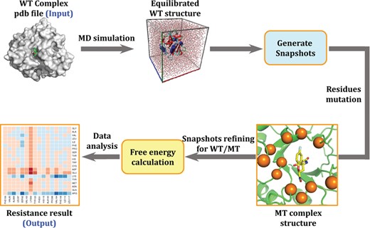
The detail of AIMMS calculation workflow. The arrows denote the computational process.
SPEC_MOD: a designated mutation module
Input: Different with SCAN_MOD, the mutation site can be assigned directly by user in this module. For convenience, the MT protein sequence(s) can be uploaded and the mutation positions will be detected automatically by this module. The sequence with multiple mutation sites is allowed. The sequence of the submitted WT protein–ligand complex structure in PARA_MOD will be used as a template for sequence alignment. Other options include task name, MD simulation settings, password and e-mail are the same with SCAN_MOD.
Workflow: The sequence alignment will be performed to confirm the mutation type(s) and site(s). Then the MD simulation will be performed. The snapshots extracted from MD trajectory are mutated and the ΔΔG value of each mutant can be obtained by using the same procedure in SCAN_MOD.
Output: The RF value, binding free energy change and resistance level of each mutant will be listed in a table. The detailed energy terms and 3D structure could also be checked by user, which is similar with SCAN_MOD.
Results and discussion
Resistance data
According to different characters of amino acid, including amino acid size, polarity and location, drug resistance mutations can be classified into three main categories. First, mutations can be divided into different sizes: large to small, small to large and equivalent to equivalent based on the number of heavy atoms. Second, mutations can also be divided into different polarity: non-polar, polar, acidic and basic groups. Third, mutations can be divided into different locations: active site mutation or non-active site mutation. The prediction on different types of mutations could help us to understand the applicability of AIMMS server in detail. Hence, we collected the mutations that are different in size, polarity and location from literature.
In total, the performance of AIMMS was assessed on 17 protein–drug systems involving 311 mutants. The published activity data, which were shown in the format of IC50, Ki or Kd value (Supplementary Data Table S1), were only used to evaluate the prediction accuracy. AIMMS performs the prediction by using a de novo strategy based on the 3D structure of ligand–receptor complex, which can be obtained by crystal or simulation. Hence, we don’t need the detailed drug information and drug profiles, such as IC50, to build statistical learning model. The final resistance was evaluated by calculating the change of binding free energy (ΔΔG, introduced in Materials and methods section) between WT complex and MT complex to evaluate the drug resistance, which is differentiated with data-driven statistical learning system. The ΔΔGexp value was calculated according to equation (3) and listed in Supplementary Data Table S1, which was used to evaluate the binding affinity change after mutation. Resistance can be divided into two classifications: a negative value means non-resistance, but a positive value means resistance. Resistance can further be divided into four classifications according to the RF: (i) no resistance, RF ≤ 1; (ii) low resistance, 1 < RF ≤ 10; (iii) middle resistance, 10 < RF ≤ 100; (iv) high resistance, RF > 100. Corresponding to it, ΔΔGexp is also divided into four levels: (i) no resistance, ΔΔGexp ≤ 0 kcal/mol; (ii) low resistance, 0 < ΔΔGexp ≤ 1.37 kcal/mol; (iii) middle resistance, 1.37 < ΔΔGexp ≤ 2.73 kcal/mol; (iv) high resistance, ΔΔGexp > 2.73 kcal/mol. We tested the prediction performance of AIMMS by two standards: the prediction accuracy of binary and four classifications. Both of the experimental resistance level (RLexp) and calculated resistance level (RLcal) were labeled for every mutant to check the prediction performance.
Performance evaluation
Overall, for the resistance or non-resistance prediction, AIMMS identified 241 out of the 264 positive samples (resistance mutants) with the sensitivity of 91.3% and 37 out of 47 negative samples (non-resistance mutants) with the specificity of 78.7%; 278 samples were correctly divided into resistance or non-resistance with the accuracy of 89.4%. To evaluate the discriminatory ability of AIMMS, the receiver operating characteristic (ROC) curve analysis was also performed between the experimental data (ΔΔGexp) and calculation result (ΔΔGcal) for resistance and non-resistance data. It shows in Figure 4 that the area under ROC curve (AUC) is 85.5%. The best critical point (true positive rate = 91.7, false positive rate = 21.3%) on the curve means that the highest possibility of a mutant to be resistant is 91.7% and a mutant to be non-resistant is 78.7%. As shown in Supplementary Data Table S2, the sensitivity and specificity of AIMMS are 91.3 and 78.7%, which are close to the highest possibility. Hence, it proves the power of the prediction ability of AIMMS.

The ROC curve showing the relationship between specificity and sensitivity on distinguishing resistance and non-resistance mutants.
Although the AUC is the most commonly used global index of prediction accuracy, the Youden index (YI) is also frequently used in practice [42]. This index can be defined as J = sensitivity + specificity − 1 and ranges from 0 to 1. Complete separation of the distributions of the marker values for the resistance and non-resistance results in J = 1 whereas complete overlap gives J = 0. The YI has an attractive feature not present in the AUC. It provides a criterion for choosing the optimal threshold and defines the maximum potential effectiveness for a classifier. According to the best critical point, the YI reached to the maximum value (0.704) with the critical ΔΔGcal = −0.005 kcal/mol, which means the performance of AIMMS will reach best by using −0.005 kcal/mol as the threshold to discriminate resistance or non-resistance. Obviously, using the critical ΔΔGcal = 0 kcal/mol as the threshold in the actual prediction, the YI can reach to the value of 0.7, which represent the ability of AIMMS to avoid misclassifications.
In addition, AIMMS showed very good performance on further resistance level prediction defined by three thresholds (low resistance, middle resistance and high resistance). The total accuracy of resistance prediction can reach to 82.6 (low resistance), 90.4 (middle resistance) and 97.4% (high resistance) (as shown in Table 1). The detailed analysis for the three resistance thresholds were shown in Supplementary Data Table S2. The sensitivity ranges from 71.0 to 90.9%, and the specificity ranges from 86 to 97.9%. In order to check the applicability of AIMMS on different protein–drug systems, the accuracy for every inhibitor was also investigated (Table 1). The accuracy of non-resistance prediction ranged from 79 to 100%, with 13 out of 17 drugs reached over 85%. Take the drug ETR for example, all of the negative samples (non-resistance) were correctly predicted to be non-resistance. A total of 10 positive samples (resistance) were wrongly predicted to be non-resistance. Hence, it results in a lower accuracy (Table 1). But 9 out of the 10 positive samples were low resistance in the experiment, which were very close to the predicted resistance level. Similarly, 11 out of 17, 13 out of 17 and 17 out of 17 drugs were predicted to be low, middle and high resistance, respectively, with accuracy over 85%. Take SQV for example, four negative samples (I50V, I54V, I84V and L10F/I84V) were wrongly predicted to be positive (low resistance); hence the prediction accuracy for SQV is the lowest (72%). However, the predicted resistance value of the four mutants is not far from the exact experimental resistance value.
The predictive accuracy for every inhibitor on all mutants under four thresholds
| Systems | Inhibitors | Mutants no. | Accuracy | |||
|---|---|---|---|---|---|---|
| Noa | Lowb | Middlec | Highd | |||
| HIV protease | APV | 13 | 1 | 0.85 | 0.77 | 0.85 |
| NFV | 8 | 1 | 1 | 1 | 1 | |
| SQV | 18 | 1 | 0.72 | 0.78 | 1 | |
| DRV | 4 | 1 | 1 | 1 | 1 | |
| LPV | 6 | 1 | 1 | 1 | 1 | |
| HIV reverse transcriptase | EFV | 45 | 0.82 | 0.76 | 0.84 | 0.93 |
| NVP | 34 | 0.88 | 0.85 | 0.94 | 0.97 | |
| RPV | 49 | 0.84 | 0.78 | 0.94 | 1 | |
| ETR | 47 | 0.79 | 0.74 | 0.89 | 1 | |
| Influenza virus neuraminidase | ZMR | 7 | 1 | 1 | 1 | 1 |
| bc1 complex | STI | 6 | 0.83 | 1 | 1 | 1 |
| DHFR-TS | CYC | 12 | 1 | 1 | 1 | 1 |
| PYR | 12 | 0.92 | 0.83 | 0.83 | 0.92 | |
| Aldose reductase | FID | 8 | 1 | 0.88 | 0.88 | 1 |
| Kinase | GEF | 5 | 1 | 1 | 1 | 1 |
| DAS | 20 | 0.95 | 0.8 | 0.9 | 1 | |
| NIL | 17 | 1 | 0.94 | 1 | 0.94 | |
| Total | 17 | 311 | 0.89 | 0.83 | 0.90 | 0.97 |
Note: The accuracy is evaluated by categorizing the mutant into anon-resistance, blow resistance, cmiddle resistance, and dhigh resistance.
In order to make a further judgment on the predictive ability of AIMMS, a comparison of the prediction accuracy between AIMMS and CMS protocol was performed. Compared with CMS, an MD simulation was added to further relax the structure of mutant in the refinement step of AIMMS, which were proved to have an improvement on the resistance prediction accuracy for all the tested samples. The average prediction accuracy only ranges from 47.0 to 72.0% according to the previous CMS protocol. However, the prediction accuracy can rise to a range of 83–97% by the introduction of MD simulation in the refinement step of CMS protocol (shown in Supplementary Data Table S3). This indicates that the binding structure between the mutant and ligand might have not been fully relaxed during the energy minimization process according to the old CMS protocol, which might significantly overestimates the binding free energy shift when the mutation causes a considerable change in the binding mode of ligand.
Meanwhile, we also investigated the prediction accuracy of the similar drug resistance prediction tools and compared with AIMMS. The prediction results associated with other similar tools were summarized in Table 2. Due to the different requirement in drug resistance study, there was not a uniform standard to evaluate drug resistance prediction accuracy. Hence, different criteria have been used as indicators to evaluate the predictive ability of these studies. Compared with other de novo prediction methods, the prediction accuracy of AIMMS is in the range of 79–100% under criterion 1 and 83–97% under criterion 2. The lowest prediction accuracy under criterion 1 and the highest prediction accuracy under criterion 2 are higher than the other methods. Most importantly, the target selection scope and number of samples are much broader and larger than other de novo prediction methods. Compared with data-driven and comprehensive prediction methods, the prediction accuracy and the target selection scope of AIMMS are still dominant. However, the tested sample numbers of data-driven methods are obviously larger than de novo prediction methods. This is because of two reasons: (1) De novo prediction is relatively more time-consuming than the data-driven methods. (2) Most of data-driven methods only perform a prediction of resistance or non-resistance, but not perform a prediction of dividing drug resistance into multiple levels, which will need more detailed activity data (such as IC50, Ki or Kd value) for validation. This is just scarce in most of these test samples. Based on the above analysis, we can infer that AIMMS keeps better or comparative predictive ability compared with these similar tools [43–49]. The detailed methods, accuracy and references were listed in Table 2.
Several computational drug resistance prediction methods compared with AIMMS
| Year | Method | Target(s)/inhibitor(s) | Prediction accuracy,a% | Sample set, mutants | Ref | ||
|---|---|---|---|---|---|---|---|
| Criterion 1 | Criterion 2 | Criterion 3 | |||||
| De novo prediction approaches (structure-based prediction approaches) | |||||||
| 2008 | MD with free energy/variability value | HIV protease/5 inhibitors | 75–100 | 33 | [43] | ||
| 2016 | Alpha shape model with MD simulation | Epidermal growth factor receptor/1 inhibitor | 90 | 30 | [44] | ||
| 2016 | Homology modeling, docking, MD simulation and MM/GBSA calculation | Topoisomerase I/7 inhibitors | 91.6b | 72 | [45] | ||
| 2017 | Docking with Molecular Mechanics Generalized Born Surface Area (MM/GBSA) calculation | ABL kinase/5 inhibitor | 70 | 55 | [46] | ||
| 2018 | AIMMS | HIV protease/5 inhibitors HIV reverse transcriptase/4 inhibitors Influenza virus neuraminidase/1 inhibitor bc1 complex/1 inhibitor, DHFR-TS/2 inhibitors Aldose reductase/1 inhibitor, kinase/3 inhibitors | 79–100 | 83–97 | 311 | ||
| Data-driven and comprehensive prediction approaches | |||||||
| 2005 | Linear regression, docking with dynamics, sequence consensus | HIV protease/6 inhibitors | 73–86 | 1792 | [47] | ||
| 2008 | Docking and multivariate statistical procedures | HIV reverse transcriptase/55 inhibitors from NIAID HIV protease/51 inhibitors from NIAID | 65–80 | 530 | [47] | ||
| 2013 | Logistic regression/random forests | HIV reverse transcriptase/5 inhibitors | 67.2–84.0 | 3133 | [48] | ||
| 2016 | Biophysics-based fitness | Dihydrofolate reductase/1 inhibitor | 85 | 21 | [49] | ||
aVarious criteria used to represent the prediction accuracy in the references cited. Criterion 1: percentage of the correctly predicted resistance into two categories. Criterion 2: percentage of the correctly predicted drug resistance into multiple levels. Criterion 3: correlation coefficient (R2) for the linear correction between the computational predictive result and the corresponding experimentally derived result. bOnly six mutant samples with experimental activity value were used here to calculate the accuracy.
cNIAID, National Institute of Allergy and Infectious Diseases.
Application examples
To evaluate the detailed usage of AIMMS web server, the Abl kinase inhibitor nilotinib was used as an example. The WT complex crystal structure (PDB ID: 3CS9) was downloaded from PDB. The activity data of the related 17 mutants (including 13 sites surrounding the inhibitor binding position) were collected from references [50, 51]. First, the ligand nilotinib was detected and the Amber force field parameter files were generated by PARA_MOD at the same time. Second, SPEC_MOD was used to generate an equilibrated MD trajectory, perform mutation scanning and calculate binding energy change. The predicted and experimental ΔΔG values of each mutant were listed in Figure 5. The resistance levels were also labeled to every mutant according to ΔΔG experimental and prediction values, respectively.
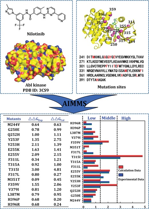
The calculation procedure and prediction result of Abl kinase inhibitor nilotinib.
As shown in Figure 5, the predicted binding free energy shifts (∆∆Gcal) are qualitatively consistent with the corresponding ∆∆Gexp values for most of the mutants (16 out of 17) in terms of the qualitative predictions of the drug resistance levels (high, middle, low or no resistance). The accuracy is ∼95%. According to Figure 5, the calculated binding free energy shifts range from 0.20 to 4.81 kcal/mol. The highest and lowest resistance levels were observed with the T315I and H396P mutants, respectively. Through a detailed analysis of the energetic data, the binding free energy changes of most mutants (G250E, Q252H, E255V, F311L, T315A, T315I, M351T, F359V, V379I and L387M) were slightly overestimated, but can be categorized to right resistance level by AIMMS. However, the Y253F mutant was identified as an outlier, with the binding free energy change overestimated by ∼1.4 kcal/mol. The experimental resistance level of Y253F is low (ΔΔGexp = 1.35 kcal/mol, RFexp = 9.62), but the calculated resistance level is high (ΔΔGcal = 2.75 kcal/mol, RFcal = 100.80). Y253 located in the active site and have a direct interaction with NIL. Hence, Y253F may lose important interaction and the original mode of inhibitor NIL binding with the enzyme may become very unfavorable. Inhibitor NIL needs to significantly change its binding mode in the binding pocket of the mutant to compensate the binding. Hence, further optimization of the mutant Y253F structure should be needed to reduce the energy overestimation.
Conclusions
In the era of precision medicine and big data, integrating bio-omics data and the clinical information will improve the identification of drug-resistant mutants. The drug resistance prediction approach plays increasingly important roles in studying the underlying mechanisms of drug resistance and in the optimal design of appropriate treatment schedule by quantitative prediction of drug administration. We presented a computational drug resistance prediction web server to perform de novo drug resistance prediction for any ligand–protein systems, which can provide solutions for both studying drug resistance mechanisms and appropriate drug administration. It is differentiated with other web services relied on a sample-driven statistical learning manner.
De novo method can predict drug resistance without resistance data; however, current available web tools are statistical learning system, which needs sufficient set of resistance data to training.
We have developed a new web tool for the prediction of drug resistance for any kind of ligand–protein system based on the structure-based mutation scanning, which represents the first automated tool for de novo drug resistance prediction.
We used many different drug–protein systems to validate the performance and compared the state-of-the-art methods with AIMMS, which keeps superior predictive ability.
Export results in multiple styles, including table, heatmap, histogram and 3D structure, for clear exhibition and better understanding.
AIMMS can be used straightforward without need of registration.
Funding
National Key R&D Program (2017YFA0505203); National Natural Science Foundation of China (21332004 and 21472060); Foundation for the Author of National Excellent Doctoral Dissertation of PR China (201472).
Feng-Xu Wu, Jing-Fang Yang, Wen Jiang, Meng-Yao Wang and Chen-Yang Jia are students at the College of Chemistry, Central China Normal University, doing a thesis in the field of computer molecular simulation.
Fan Wang is a postdoctoral fellow at the College of Chemistry, Central China Normal University. He received his PhD degree in computational chemistry from the University of Amiens, France.
Ge-Fei Hao is a professor in bioinformatics at the College of Chemistry, Central China Normal University. He received his PhD degree in pesticide science from the Central China Normal University.
Guang-Fu Yang is a professor in chemical biology. He is the group leader and has been the dean at the College of Chemistry, Central China Normal University. He received his PhD degree in pesticide science from the Nankai University, Tianjin, China.
