


Abstract
Restriction site-associated DNA sequencing (RADseq) is a powerful technology that has been extensively applied in population genetics, phylogenetics and genetic mapping. Although many software packages are available for ecological and evolutionary studies, a few effective tools are available for extracting genotype data with RADseq for genetic mapping, a prerequisite for quantitative trait locus mapping, comparative genomics and genome scaffold assembly. Here, we present an integrated pipeline called gmRAD for generating single nucleotide polymorphism (SNP) genotypes from RADseq data, de novo, across a genetic mapping population derived by crossing two parents. As an analytical strategy, the software takes five steps to implement the whole algorithms, including clustering the first (forward) reads of each parent, building two parental references, generating parental SNP catalogs, calling SNP genotypes across all individuals and filtering the genotype data for genetic linkage mapping. All the steps can be completed with a simple command line, but they can be also performed optionally if prerequisite files are available. To validate its application, we also performed a real data analysis with RADseq data from an F1 hybrid population derived by crossing Populus deltoides and Populus simonii. The software gmRAD is freely available at https://github.com/tongchf/gmRAD.
Introduction
Genetic mapping in plants and animals is especially important for quantitative trait locus (QTL) mapping [1, 2], comparative genomics [3, 4] and genome scaffold assembly [5–7]. A genetic linkage map of an organism shows numerous molecular markers on chromosomes in a linear order with genetic distances between adjacent markers. To construct a genetic linkage map, researchers must first establish a mapping population by crossing two parents, which is commonly known as a backcross (BC) or an F2 population in inbred lines [8, 9] or an F1 hybrid population in outbred species [10, 11]. Then, a large number of molecular markers must be obtained for linkage analysis across many individuals in the population. Traditionally, the molecular markers used for genetic mapping mainly include randomly amplified polymorphic DNA, restriction fragment length polymorphism, amplified fragment length polymorphisms and simple sequence repeat. These markers have the limitation of low throughput because of instability and intensive labor, mostly leading to sparse linkage maps especially in outbred species [12]. However, recent advances in the reduced-representation sequencing (RRS) technologies have revolutionized the studies of genetic mapping, allowing one to obtain hundreds or thousands of single nucleotide polymorphisms (SNPs) across the mapping population in a fast and cost-effective way for constructing genetic linkage maps [12–16].
In the past decade, a variety of RRS approaches have been developed and extensively applied in population genetics, phylogenetics and genetic mapping [17, 18]. Baird et al. [19] initially proposed the protocol for restriction site-associated DNA sequencing (RADseq) technology. This approach generally uses Illumina platforms to generate paired-end (PE) reads at specific regions near the restriction enzyme cut sites across genomes of many individuals. Since then, a series of modified approaches have emerged, such as genotyping-by-sequencing (GBS) [20], double-digest RAD sequencing [21] and specific length amplified fragment sequencing [22]. Scheben et al. [23] summarized that there were at least 13 such methods available for RRS. These methods have a common characteristic of using enzymes to digest the genomic DNA at the first step but typically differ in the number (one or two) and type of enzymes used and the steps of random shearing and size selection [23, 24]. Although the term ‘GBS’ was popularly used for describing the general RRS, Andrews et al. [17] deemed that ‘RADseq’ should be used because it captures the feature of RRS. Although high-throughput sequence data are easily available with RADseq, great challenges still exist for SNP discovery and genotyping across multiple individuals in a mapping population.
Currently, several software pipelines are available for analyzing RADseq data to call SNPs at a population level, including Stacks [18, 25, 26], PyRAD [27], TASSEL-GBS [28], AftrRAD [29], dDocent [30] and Rainbow [31]. Most of these programs focus on populations for ecological and evolutionary studies, whereas Stacks is the only software used to perform RADseq analysis for genetic mapping studies. Stacks can use RADseq data to discover SNPs for many individuals in a mapping population, either de novo or by a method based on a reference genome. This software can also export marker data formatted as input to software, such as JoinMap [32] and OneMap [33], for downstream linkage analysis and mapping. However, when performing de novo analysis for genetic mapping, the previous versions (≤1.48) of Stacks use the consensus of the stacks as the reference sequences to call SNPs but cannot utilize the contigs that could be assembled from the second RADseq reads if randomly sheared [18]. Although the latest version (2.2) supports PE reads, it seems likely that the new version has lost the function for a genetic map because (i) the program denovo_map.pl no longer has the option for a cross type such as `CP’, `F2’ and `BC1’; (ii) the program `genotypes’ is missed which was used to identify mappable loci in the previous versions; and (iii) the other programs as well as its manual on the website have no information about this feature. In addition, the software cannot handle reads of different lengths within or between samples (see its website). These drawbacks could decrease the effectiveness and extensiveness of its applications with general RADseq data in generating marker genotypes for genetic mapping.
Here, we report an integrated pipeline called gmRAD for generating SNP genotypes de novo across a genetic mapping population with RADseq data. The software involves five steps for analyzing RADseq PE reads, but one can finish the entire analysis by just inputting a command line. First, gmRAD categorizes the first (forward) RADseq reads from each parent into clusters. Second, the corresponding second (reverse) reads within a cluster are assembled into a contig, which is joined with the consensus of the first reads to form a reference sequence for the cluster. Third, SNPs are called by mapping two parental PE reads separately to one parental reference and merged into an SNP catalog. Fourth, SNP genotypes of each individual are called according to one parental SNP catalog through the procedure of mapping reads to the reference sequences. Finally, genotype data sets for genetic linkage analysis are generated by filtering the SNP genotypes according to the segregation patterns, Mendel’s law of segregation and missing genotypes in the whole mapping population. The final genotype data set can be formatted as input for the widely used genetic mapping software JoinMap [32]. To validate the software, we performed a real RADseq data analysis with gmRAD, where 6497 high-quality SNPs were successfully generated across 2 parents and 150 progeny in an F1 hybrid population of Populus deltoides and Populus simonii, leading to two perfectly constructed parental linkage maps. Our software provides a user-friendly and powerful tool to extract SNP genotype data from RADseq data for performing genetic linkage mapping in a hybrid population. The software gmRAD is freely available at https://github.com/tongchf/gmRAD.
Methods
Clustering the first reads of each parent
In order to discover SNP genotypes de novo with RADseq data from a mapping population, we categorize the first reads of the PE reads from each parent into clusters. Generally, the process of RADseq involves one or two enzymes to digest the genomic DNA, resulting in the first reads containing several bases of the enzyme footprint (e.g. ‘AATTC’ in EcolRI). Moreover, the raw PE reads usually contain primer/adaptor sequence and multiple identifier (MID) bases assigned to each sample [19]. We assumed that researchers or sequencing companies have removed the primer/adaptor sequences and segregated the reads for each sample by MID. This filtering process could be conducted with some free programs, such as process_radtags in Stacks [18]. In addition, we recommend to further filter the data for high-quality reads, using tools like the NGS QC toolkit [34]. After these quality control procedures, the first reads of each parent are first grouped into stacks with hashing algorithms to save the computing time, and then these stacks are classified into clusters, allowing a hamming distance of |${\mathrm{d}}_{\mathrm{h}}$| within a cluster as proposed in [35]. The latter procedure can be easily implemented by counting the variant nucleotides at the same position between any two sequences.
Building the reference sequences of each parent
For each parent, if the number of reads in a cluster is between a minimum and maximum value, we will try to assemble the corresponding second reads within the cluster into a contig. The minimum value is generally set to 4 or 5 as described in [35], while the maximum is taken as the quantile of the distribution of the number of reads in the cluster, which corresponds to the proportion of non-repeat sequences to the whole genome. Setting the maximum number of reads in a cluster for local assembly is to avoid assembling those reads from repeat regions on genome. The assembly step will be conducted by considering different parameters, such as overlap length, percent of mismatches and seed size, to obtain an optimal assembly result. The longest contig of the second reads will be joined with the consensus of the first reads if they have an overlap region; otherwise, they will be concatenated with 10 ‘N’. All the local sequences of each parent, generated by the assembling and joining procedures, will be used as reference sequences for calling SNPs across the mapping population independently.
Generating two parental SNP catalogs
Before calling SNP genotypes at a large number of loci for many individuals in the population, we first align the PE reads of each parent using the software BWA [36] to the female reference sequences, generating a SAM format file [37]. Then, each SAM file is filtered, such that, the remaining reads in the file satisfy the following four conditions: (1) the read or its mate must be mapped to the first position of a local reference sequence; (2) the edit distance of the mapped read is less than or equal to a preset value of |${\mathrm{d}}_{\mathrm{e}}$|; (3) the best alignment score of the read is greater than or equal to the minimum score (i.e. its length minus 5 |${\mathrm{d}}_{\mathrm{e}}$|) in the case when a mapped read has the maximum edit distance of |${\mathrm{d}}_{\mathrm{e}}$|; and (4) the best alignment score is greater than the second-best alignment score. Next, the filtered SAM files are converted to the BAM format using the sorting and indexing procedures of SAMtools [37]. Subsequently, a BCF file is produced with the BAM file using SAMtools, and it is then used to generate a VCF file with BCFtools (accompanies SAMtools) for each parent. Finally, the VCF files are filtered, such that each SNP has a mapping quality score of at least 30, and each allele of the SNP genotype has a read coverage depth of at least 3. The filtered SNPs from both parents are merged into an SNP catalog for calling the SNP genotypes of all progeny in the next step. This SNP catalog is generated on the basis of the female reference sequences, and we call it the female-based SNP catalog. In the same way, we also generate the male-based SNP catalog with the male reference sequences.
Calling SNP genotypes across a mapping population
First, with the female reference sequences generated in the building step and the female-based SNP catalog, we will call SNP genotypes for all progeny in the mapping population. The procedures are basically similar to those in calling parental SNP catalogs as described above, but there are a few differences. After the procedure from mapping the PE reads to generating a BCF file for each progeny, the BCF file is used to generate a VCF file according to the SNP catalog with SAMtools. From the VCF file, an SNP genotype file for the progeny is extracted, such that the read coverage of an allele is not less than |$c$| (≥3) for a heterozygote and 5 for a homozygote, while the other parameters are the same as those used for calling parental genotypes. Next, all the SNP genotype files are merged into one SNP file, where each line contains an SNP site information and the genotypes of the two parents and all progeny. This SNP genotype data set, generated on the basis of the female reference sequences, is denoted as FD. Using the same procedures, we will generate another SNP genotype data set, denoted as MD, based on the male reference sequences and the male-based SNP catalog.
Filtering SNP genotype data for linkage analysis and mapping
The two SNP genotype files generally include a large number of SNP sites, but only those SNPs that segregate as per Mendel’s law and have no or only a few missing genotypes in the population are used for the downstream genetic mapping study. For each segregating SNP site, we mark its segregation type as aa×ab, ab×aa, ab×ab, ab×cd, aa×bc, ab×cc or ab×ac, where the first two letters of each type denote the maternal genotype and the last two the paternal genotype. After counting the progeny number for each genotype at a fixed segregation site, a chi-squared test is performed for that site, and the P-value is calculated. If the P-value is greater than 0.01 and the percent of missing genotypes is less than the threshold (e.g. 10%), then the record of that SNP is saved in a new data set for further analysis. As a result, the previous SNP genotype data sets FD and MD are filtered into two new data sets, namely FD1 and MD1, respectively. As proposed by Mousavi et al. [12], the identical SNPs between FD1 and MD1 are chosen for linkage mapping, at which the genotypes in the two data sets are the same across all individuals. These identical SNP genotype data for each segregation type are saved in a separate text file. In addition, an Excel file is generated to be used as input in JoinMap that converts the segregation types of aa×ab and aa×bc to nn×np, ab×aa and ab×cc to lm×ll, ab×ab to hk×hk and ab×ac to ef×eg.
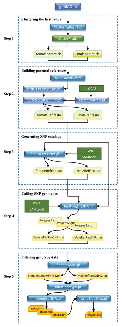
Schematic representation of the work flow of the gmRAD software. Five steps are taken in running gmRAD: clustering the first reads, building the parental reference sequences, generating parental SNP catalogs, calling SNP genotypes for all individuals and filtering genotype data. The rectangles with rounded corners indicate in-house programs written in Perl (blue) and C++ (green). The normal green rectangles indicate the external packages used in gmRAD, including BWA, SAMtools and LOCAS. The cut-corner rectangles indicate the intermediate and final result text files.
Implementation
We developed an integrated package called gmRAD to implement our strategy for generating SNP genotypes in a mapping population. The package was written in Perl and C++ and combined several available tools such as LOCAS (http://ab.inf.uni-tuebingen.de/software/locas/), BWA [36] and SAMtools [37]. Like most large assemblers such as ALLPATHS and SOAPdenovo [38, 39], LOCAS used a de Bruijn graph algorithm to build contigs, but its scale was so small that it could be suitably applied in gmRAD. As a main program, gmRAD.pl takes five steps to implement all the algorithms, which include clustering the first reads of RADseq data, building two parental reference sequences, generating two parental SNP catalogs, calling SNP genotypes for all individuals and filtering SNP data for practical linkage mapping (Figure 1). These steps can be finished at one time, can also be performed independently if the prerequisite files are available. The clustering step uses the Perl program clusteringRead1.pl through calling the two C++ programs of clusterRead1 and merge2Cls to generate the first read clusters for each parent. In the step for building parental reference, gmRAD uses the Perl program buildParentRef.pl, with the three core Perl scripts (callR1ClsConsensus.pl, assemblR2Cls.pl and joinR1consR2contig.pl), to produce the consensus of the first reads and the contig of the corresponding second reads and joins them to form a local reference for a cluster. To obtain the longest contig of the second reads, gmRAD uses the program LOCAS for assembly, by choosing multiple values of different parameters. For the female parental reference sequences, the step for generating SNP catalogs uses the Perl program findParentsSNPs.pl to derive the SNP sites with reads from each parent independently, and these SNPs are merged as an SNP catalog to call SNP genotypes for all progeny. Then, gmRAD uses the Perl program findProgenySNP.pl to call SNP genotypes of all progeny based on one maternal reference and SNP catalog. During this step, the famous software packages BWA and SAMtools are used for reads mapping and SNP calling. After the completion of the calling step, an SNP genotype data set across all individuals is generated on the basis of the maternal reference sequences. Following the same steps, another SNP genotype data set is also generated on the basis of the paternal reference sequences. In the last step for filtering SNP data, gmRAD extracts SNP genotype data across all individuals for genetic mapping analysis with the Perl programs filterRawSNP.pl, filterGenotype.pl, findIdenticalSNPs.pl and write2JoinMap.pl. The program filterRawSNP.pl identifies the segregation type, counts the individual number of genotypes and calculates the P-value for testing whether the SNP follows the Mendel’s law of segregation for each SNP in both the SNP genotype data sets generated above. Next, the program filterGenotype.pl classifies each filtered data set into different segregation type files on the basis of the threshold values of missing genotype rate and P-value. Then, the program findIdenticalSNPs.pl finds the identical SNP data set of each segregation type from the same segregation type files generated by the program filterGenotype.pl. These identical SNP data set files are prefixed with the corresponding segregation notations such as aa×ab, ab×ab and ab×cd. Finally, using the program write2JoinMap.pl, an additional file including all types of identical SNPs is generated in Excel format, to be used as input in JoinMap. The work flow of all the programs including the external packages used in gmRAD is depicted in Figure 1.
Results
The software and its usage
The newly developed software gmRAD is freely available at https://github.com/tongchf/gmRAD and can be run under Linux systems. To run gmRAD, users have to download and install the external packages in advance, including LOCAS, BWA [36], SAMtools and BCFtools [37] and a parameter setting file named ‘parameters.ini’ must be created (Figure 2). The parameter file consists of three parts, folders, parameters and fastq files. In each part, every non-comment line starts with a string, generally in capitals, as a variable in gmRAD, followed by a colon and space, and then one or two strings as a value of the variable. The first part ‘folders’ gives the software paths of gmRAD itself, LOCAS, BWA, SAMtools and BCFtools as well as the path where the fastq data files of the two parents and all their progeny are saved. The second part ‘parameters’ includes the number of threads used for parallel computing, the hamming distance for clustering the first reads, the edit distance for filtering mapped reads, the read coverage depth of an allele of a heterozygote, the estimated percent of genome repeat regions, the minimum score of an SNP genotype, the percent of non-missing genotypes required and the minimum P-value allowed for testing the segregation ratio at an SNP site. The third part ‘fastq files’ presents the first and second read files of all individuals, including the two parents.
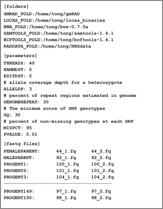
The style of the parameter setting file for launching gmRAD.
Once the external packages are installed and the parameter file is prepared, users can finish the whole computing work for extracting SNP genotype data by running gmRAD with just a command-line ‘perl gmRAD.pl’. However, users can run gmRAD for a specific step by skipping other four steps if the prerequisite files are already available. A test data is provided online for users to quickly grasp how to use gmRAD. The data includes the first and second reads files for 2 parents and 20 progeny samples. During the computing processes, a series of temporary files or folders will be generated, some of which are the prerequisite files for the next step of the analysis. Table 1 lists the prerequisite files and main result files for every analytical step. It is not difficult for the users to understand the contents of these files, with the descriptions in the Methods and Table 1 making it simpler.
The prerequisite files for running each of the five analysis steps in gmRAD with default parameters and the corresponding main result files each with a description.
| Step | Prerequisite Files | Main Result Files | Description |
|---|---|---|---|
| 1 | parameter.ini | femaleparent.cls | The first read ids and their consensus within a cluster for the female parent. |
| maleparent.cls | The similar file for the male parent. | ||
| 2 | parameter.ini | femaleClusterRef.fasta | The reference sequences built from the first and second reads within each cluster for the female parent. |
| femaleparent.cls | |||
| maleparent.cls | femaleClusterRef.fasta | The similar file for the male parent. | |
| 3 | parameter.ini | female_gtp.loc | SNP catalog based on the female reference. |
| femaleClusterRef.fasta | female.gtp | The female and male genotypes based on the female reference. | |
| maleClusterRef.fasta | male_gtp.loc | SNP catalog based on the female reference | |
| male.gtp | The female and male genotypes based on the male reference. | ||
| 4 | parameter.ini | FemaleRefRawSNPs.txt | SNP genotypes across all individuals based on the female reference. |
| female.gtp | |||
| female_gtp.loc | MaleRefRawSNPs.txt | SNP genotypes across all individuals based on the male reference | |
| male.gtp | |||
| male_gtp.loc | |||
| 5 | parameter.ini | FemaleRefRawSNPs2.txt | Genotype counts, p values for chi-squared test and genotype notations for each record in |
| FemaleRefRawSNPs.txt | FemaleRefRawSNPs.txt. | ||
| MaleRefRawSNPs.txt | MaleRefRawSNPs2.txt | The similar file from MaleRefRawSNPs.txt. | |
| aaxab_pct90pv01.txt | The final genotype data segregating in aaxab. | ||
| aaxbc_pct90pv01.txt | The final genotype data segregating in aaxbc. | ||
| abxaa_pct90pv01.txt | The final genotype data segregating in abxaa. | ||
| abxab_pct90pv01.txt | The final genotype data segregating in abxab. | ||
| abxac_pct90pv01.txt | The final genotype data segregating in abxac. | ||
| abxcc_pct90pv01.txt | The final genotype data segregating in abxcc. | ||
| abxcd_pct90pv01.txt | The final genotype data segregating in abxcd | ||
| all_pct90pv01_joinmap.xlsx | All final genotype data formatted as input to the software JoinMap. |
A real example
We performed a real data analysis to demonstrate that gmRAD is a powerful tool in calling SNP genotypes with RADseq data for genetic linkage mapping. The RADseq data was generated from an F1 hybrid population of P. deltoides and P. simonii by sequencing the 2 parents and their 150 progeny at Beijing Genomics Institute (BGI), Shenzhen, China [12]. Unlike in inbred lines, an F1 hybrid population was often chosen as a genetic mapping material in forest trees because of their high heterozygosity and long generation times. We had established this mapping population of Populus in 2011 and then focused on studies of genetic linkage mapping and QTL locating with this material [12, 16, 40, 41]. The raw data was deposited with accession number SRP052929 at the NCBI SRA database. The accession number prefixed with SRR for the individual reads file is given in Supplementary Table S1. After filtering with the NGS QC toolkit using the default parameters [34], these RADseq data were used to call SNP genotypes with gmRAD by setting the parameter values as shown in Figure 2.
The first reads of the female parent P. deltoides were grouped with a hamming distance of 5. By excluding the clusters with a small or large number of reads, 214 511 clusters were obtained, each containing 5–258 reads. The upper bound of the read numbers was determined by the ratio of repeat genome regions estimated from the reference genome of Populus trichocarpa [42], and by considering that the reads in reads-rich clusters are from the repeat genome regions. In the same way, 220 448 clusters were derived from the first reads of the male parent P. simonii, each containing 5–1450 reads. Each cluster of the two parents was used to build a RAD tag sequence by joining the consensus of the first reads and the contig of the second reads. Consequently, 209 681 and 217 007 RAD tag sequences were obtained from the female and male parents, respectively. These RAD tag sequences from each parent were taken as reference sequences to call SNP genotypes across all individuals including the two parents, resulting in two SNP genotype data sets each on the basis of one parental genome. Furthermore, the SNP genotypes across all progeny were filtered by removing those SNP sites that had more than 5% missing genotypes and a P-value less than 0.01. Finally, an identical SNP genotype data set, for the two filtered SNP genotype data sets generated above, was derived (see Methods). The final identical genotype data were categorized and saved according to their segregation types. An additional file that contained all kinds of segregation genotype data was formatted to be used as input in JoinMap. The whole computation was finished on a high-performance computer with four CPUs (AMD Opteron 6386 SE) and 256 GB of RAM, totally speeding about 3 days and 4 h, with 2 h for clustering the first reads, 45 h for building the parental references, 8 h for generating the SNP catalogs, 20 h for calling progeny SNP genotypes and 1 h for filtering the genotype data.
In order to demonstrate the practical use of the data generated with gmRAD, we used the two final identical SNP data sets with segregation types of ab×aa and aa×ab to construct the two parental genetic linkage maps. As a result, each of the two SNP data sets were classified into 19 linkage groups under a wide range of logarithm of odds (LOD) thresholds (9–16 for ab×aa and 6–22 for aa×ab), which perfectly matches the karyotype of Populus. The maternal linkage maps contained 3913 SNPs and spanned 5688.15 cM with an average genetic distance of 1.46 cM between adjacent SNPs, and the paternal linkage maps consisted of 2584 SNPs with a total genetic distance of 5244.46 cM and an average of 2.04 cM (Supplementary Figures S1 and S2).
To compare the performance of gmRAD with Stacks, we generated genetic markers with the same RADseq data using the program denovo_map.pl with parameter values of m3, M5 and defaults for the others in Stacks. The parameter values of m and M were not only respectively equal to the depth of alleles and the hamming or edit distance used in the analysis with gmRAD but also matched the optimal values for analyzing data set TRT in [43]. Since Stacks cannot handle different lengths of reads, we trimmed the first reads of each sample to the minimum length of 82 bp (Supplementary Table S1). We performed the analysis for the two data sets of the first and second reads separately. It took about 1 day to finish the computing for each data set. After completing the computation, we filtered the marker loci according to the thresholds of missing genotype rate and P-value, as used in the analysis with gmRAD and then removed the redundant loci, i.e. kept one locus among all completely linked loci. Consequently, we obtained 2379 marker loci segregating in ab×aa and 1676 as aa×ab, which was 39.20 and 35.14% less than the numbers of SNPs generated with gmRAD, respectively. For the markers segregating in ab×aa, 19 maternal linkage groups were constructed under the LOD thresholds from 5 to 20, with a total genetic distance of 3151.01 cM and an average interval distance of 1.34 cM (Supplementary Figure S3). Similarly, the markers segregating in aa×ab were also classified into 19 paternal linkage groups under the LOD thresholds from 5 to 17, with a total genetic distance of 3678.21 cM and an average interval distance of 2.22 cM (Supplementary Figure S4).
To evaluate the accuracy of calling genotypes with gmRAD and Stacks, three individuals, including the two parents and one progeny (field ID: ‘C15–1’), were used to validate the genotypes by sequencing each sample independently at BGI and Novogene Bioinformatics Institute (NBI; Beijing, China), as we had performed before [16]. The genotypes were limited to the marker loci generated above with gmRAD or Stacks. For each individual, we counted the loci at which the genotypes were successfully called not only with the data from BGI but also from NBI. Meanwhile, the number of loci at which the genotypes were confirmed consistently with the data from the two different companies was also recorded. Thus, the rate of consistent genotype loci was easily inferred from the two counts for each individual and can be regarded as a measure of accuracy for the software, gmRAD or Stacks, in generating genetic markers. These results are presented in Supplementary Table S2. It can be seen that both the tools have very high consistent genotype rate (>96%), but Stacks was more accurate compared to gmRAD by >1.26–2.48%. As expected, the accuracy of gmRAD can be improved by increasing the value of parameter ‘ALLELDP’ in ‘parameters.ini’. When we changed the parameter value from 3 to 5, we performed the analysis of our real data set with gmRAD again and obtained 4623 SNPs segregating in aa×ab or ab×aa, which was 14% more than the number (4055) generated with Stacks. In the same way, the rate of accuracy was estimated to be >98% for the three samples, increasing by 0.75–1.90% (Supplementary Table S2).
Discussion
We provided a powerful software package, gmRAD, to generate SNP genotype data for genetic linkage mapping with RADseq data from two parents and their progeny in a hybrid population. The novel software is a convenient tool for users to complete the whole computation by inputting only one command line and can handle a broad range of PE reads from RADseq, but the five analytical steps involved can be independently run if some prerequisite data are available. The first two algorithm steps of gmRAD include clustering and assembling the PE reads from the two parents separately, which were initially proposed by Willing et al. [35]; however, they had used the merged PE reads from all the six samples for clustering and assembling. To join the consensus of the first reads and the contig of the second reads within a cluster, we wrote the Perl program namely ‘joinR1consR2contig.pl’. The step for SNP calling in gmRAD is almost similar to the strategy described by Mousavi et al. [12], which was based on the generation of two genotype data sets from the respective parental references and find the identical SNPs between them as the final mapping markers. However, in gmRAD the parental references are derived just from the RADseq data of the parents, while in the previous study [12] the parental references were assembled with the whole genome sequencing data. The filtering step gives the SNP genotype data with default parameters, i.e. permitting 10% missing genotypes and taking the threshold P-value as 0.01. Users can use different parameters to filter the SNP genotype data with the Perl programs ‘filterGenotype.pl’ and ‘findIdenticalSNPs.pl’ in gmRAD according to their practical requirements. In summary, as an integrated package, gmRAD has implemented the complicated procedures to extract SNP genotypes from RADseq data but can be easily manipulated in practice. In addition, we have demonstrated its validation with a real example, in which gmRAD generated more SNP markers with the same RADseq data than in the previous study [12] for constructing the linkage maps of P. deltoides and P. simonii, and these markers of each segregation type were also classified into 19 linkage groups under a large range of LOD thresholds, perfectly matching the karyotype of Populus (Supplementary Figures S1 and S2).
The main advantage of gmRAD is that it can generate a greater number of high-quality SNP markers than Stacks using RADseq data for genetic mapping. In the real example, gmRAD generated ~60% more marker loci than Stacks (6497 versus 4055) in both segregation types of ab×aa and aa×ab. It can generate SNPs not only from the first reads but also from the second reads; here, ∼85% (5516) SNPs were located in the consensus of first reads and ∼15% in the contigs assembled from second reads. Therefore, even if we limit the SNPs from the first reads, the number is ∼36% (5516 versus 4055) greater than that generated with Stacks. In contrast, Stacks extracted the marker loci just from the first reads, because the second reads were randomly positioned and cannot easily form stacks for most samples. As for the accuracy of marker genotypes, gmRAD was less accurate compared to Stacks (see Results). This may be because of generating many more SNPs, but the estimated consistent genotype rates for the three individuals were >96%, which is an extremely high rate. However, the accuracy of gmRAD can be improved by increasing the allele coverage depth set in the parameter file (Supplementary Table S2). The ability of gmRAD to generate more number of SNPs, but with a high level of accuracy, may be due to its strategy of de novo SNP discovery. gmRAD uses each parental reference to generate two SNP genotype data sets and finds the identical SNPs for genetic mapping. This method can obtain high-quality SNP data because the two SNP genotype data sets generated on the basis of each parental reference can validate each other across the mapping population and make each identical SNP data substantially correct. This strategy was successfully implemented in our previous work [12], where the parental references were generated from whole genome sequencing and not from RADseq.
As to the choices of the hamming distance for clustering the first reads and the edit distance for filtering mapped reads in a SAM file, users can set their values within a range of 3–8 in the parameter file. For the hamming distance, a reasonable principle can be followed to choose an optimal value such that the number of the clusters generated under it is approximately equal to two times the number of the restriction enzyme cut sites on an available reference genome. This can be implemented by testing several values with the first step of gmRAD. However, this approach is a little more complicated and thus is not suitable for most researchers. Alternatively, users could set a small value for the hamming distance (e.g. 4 or 5). This would increase the number of clusters and hence lead to some redundant reference sequences in the building step, which originate from homologous regions on genome. The redundant sequences could generate redundant SNP sites, but they would be filtered as SNP bins at the last step in gmRAD. Therefore, a small value of the hamming distance should not substantially affect the final results. As for the edit distance, we set the value such that the reads remained in the filtered SAM file have a relatively high score for the best alignment. For example, if the edit distance is set to 4 and a mapped read length is 80 bp, the threshold for filtering is 60 (80 – 4 × 5). That is to say, if the best alignment score of the mapped read is less than 60, gmRAD will remove this read for the analysis in the next steps.
The utilization of the final identical SNP data, derived with gmRAD for genetic mapping, is an essential issue that needs to be addressed. In our experience ([12, 16] and the example in this study), when the majority of SNPs segregate in the types of ab×aa and aa×ab, two separate parental linkage maps should be constructed containing the respective segregation data since the SNP segregating in ab×aa has no linkage information with the others segregating in aa×ab. If the fully informative SNPs that segregate in ab×ab or ab×cd are enough available, an integrated linkage map can be constructed for both parents with the SNPs segregating in 1:1 ratio. This strategy is used for constructing linkage maps in a hybrid F1 population derived by crossing two parents in outbred species, generally using software, such as JoinMap [32], OneMap [33] and FsLinkageMap [44]. Meanwhile, gmRAD can also be applied to generate SNP markers for mapping BC and F2populations, which are derived from inbred lines. However, only the SNPs segregating in ab×aa or aa×ab are used for BC population, while the SNPs segregating in ab×ab are used for F2. Although the traditional linkage analysis tool MapMaker [45] is usually used for BC and F2 populations where the linkage phases are considered to be fixed, a genetic mapping software designed for an F1 hybrid population is recommended because the linkage phases in such populations may not always be fixed under the level of SNPs.
Once the types of SNPs for the genetic mapping are determined, the data characteristics should be considered to improve the accuracy and quality of the linkage maps, including the missing genotype rate and the threshold of P-value for filtering out the seriously distorted markers. If the filtered SNPs are categorized into linkage groups and the number of linkage groups is fixed under a large range of LOD thresholds and particularly matches the karyotype of the species studied, the data are considered to be perfect for genetic mapping. In the real example of this study, the 3913 SNPs for constructing the maternal genetic maps were classified into 19 linkage groups under the LOD thresholds from 9 to 16 and the group number is perfectly equal to the karyotype of Populus. In addition, the same characteristics are shared by the 2584 SNPs that were used to build the paternal genetic maps. In order to obtain such good data sets, the SNP data should be filtered by adjusting the percent of missing genotypes and the P-value threshold. Adjusting the percent of missing genotypes by fixing the P-value at 0.01 in the filtering process is recommended. We found that if the missing genotype rate is decreased, the number of linkage groups could not be stable within a wide range of LOD thresholds. This may occur because some of the continuously distributed SNPs are possibly removed to enable the classification of the SNPs on the same chromosome into two or more linkage groups, even with a lower LOD threshold.
A novel software package was described for calling SNP genotypes with RADseq data across many individuals in a hybrid population for constructing genetic linkage maps.
The package gmRAD involves five steps for implementing the whole algorithm, all of which can be finished smoothly by inputting a simple command line, but each step can be performed independently if the prerequisite files are available.
gmRAD can obtain high-quality SNP data through a strategy where two SNP genotype data sets are first generated on the basis of each parental reference, and then the identical SNPs are found between the two across all individual genotypes, which forms the final data set.
gmRAD provides a useful function to flexibly filter the SNPs used for constructing perfect genetic maps, particularly making the number of linkage groups to match the karyotype of the species studied.
Funding
National Natural Science Foundation of China (31870654 and 31270706); Priority Academic Program Development of the Jiangsu Higher Education Institutions.
Dan Yao is a Master’s student at the Southern Modern Forestry Collaborative Innovation Center, College of Forestry, Nanjing Forestry University, Nanjing 210037, China.
Hainan Wu is a Master’s student at the Southern Modern Forestry Collaborative Innovation Center, College of Forestry, Nanjing Forestry University, Nanjing 210037, China.
Yuhua Chen is a PhD student at the Southern Modern Forestry Collaborative Innovation Center, College of Forestry, Nanjing Forestry University, Nanjing 210037, China.
Wenguo Yang is a PhD student at the Southern Modern Forestry Collaborative Innovation Center, College of Forestry, Nanjing Forestry University, Nanjing 210037, China.
Hua Gao is a PhD student at the Southern Modern Forestry Collaborative Innovation Center, College of Forestry, Nanjing Forestry University, Nanjing 210037, China.
Chunfa Tong is Professor of Forest Genetics and Tree Breeding at the Southern Modern Forestry Collaborative Innovation Center, College of Forestry, Nanjing Forestry University, Nanjing 210037, China.
References
