


ABSTRACT
The Striped Bass Morone saxatilis is an anadromous fish that has experienced population declines and recoveries throughout its range from the 1960s to the present day. While many United States fisheries have reopened since the most recent declines, ongoing monitoring is required to ensure that numbers remain stable in the long term. Central to this is the need to determine the extent to which major spawning locations contribute to coastal stocks. While next-generation genomic sequencing can discriminate among closely related breeding aggregations within the Striped Bass native range, the cost per sample of next-generation sequencing methods currently used is too high to be applied to large-scale and long-term projects moving forward.
We developed, optimized, and evaluated a GT-Seq panel—a small panel of highly informative single nucleotide polymorphisms—capable of assigning large numbers of Striped Bass to six genetically distinct regions across the Striped Bass spawning range at much lower cost than the previous next-generation sequencing methods.
The final panel of 233 loci was able to assign 95% of reference individuals to region of origin and had <5% error across all simulations when estimating the mixing proportion of any stock.
This panel is being used in ongoing characterizations of Striped Bass along the Massachusetts coast and the eastern coast of Nova Scotia. For researchers tracking the migration of Striped Bass throughout their native range, this panel provides a low-cost method of genetically characterizing stocks at specific locations and times that can be easily modified or updated as additional, new genetic data become available.
Lay Summary
We created a genetic tool that allows Striped Bass to be assigned to a region of origin in a cost-effective and easy way, providing a tool to solve a long-standing data need for the species.
INTRODUCTION
Highly migratory fish such as salmonids, tuna Thunnus spp., and billfishes (family Istiophoridae) present unique challenges to management and monitoring. Migration routes for these species often span large distances and cross geopolitical boundaries, requiring cooperation among multiple organizational bodies to manage a single species (Miller, 2007; Nikolic et al., 2017). As well, marine aggregations of fish often contain individuals from multiple spawning populations of different productivity levels, such that fishing pressure on these mixed stocks can impact mortality rates of multiple spawning populations to different extents (Crozier et al., 2004; Staton et al., 2020). Uncertainty in the proportion of spawning populations represented in a mixed stock at a given time complicates attempts to determine fishing pressure on individual populations (Adkison, 2022; Crozier et al., 2004). Knowledge of migration ecology in these highly migratory species is therefore crucial for accurately assessing mortality in marine environments and estimating the impact on recruitment and stock biomass in future years (Reid et al., 2023; Staton et al., 2020).
One such migratory species is the Striped Bass Morone saxatilis. The Striped Bass is an anadromous fish that supports fisheries in freshwater rivers, large estuaries, and ocean habitats along the North American Atlantic coast. Its native range extends from the St. Lawrence River in Canada to the Gulf of Mexico (Setzler et al., 1980; Wirgin et al., 2005). Striped Bass populations throughout their native range have suffered from population declines in the last century, resulting in increased monitoring and management of fishing intensity. Following population crashes throughout the native range in the 1960s through 1980s (Carmichael et al., 1998; Richards & Rago, 1999), strict fishing moratoriums and quotas were implemented and resulted in recovery of many (but not all) major populations from 1995 through the present day (Atlantic States Marine Fisheries Commission [ASMFC], 2013; Fisheries and Oceans Canada, 2018; Richards & Rago, 1999). Despite this recovery, careful observation and management of Striped Bass fisheries continues to ensure that populations remain stable and recovery is long term (ASMFC, 2022a). The United States migratory stock of Striped Bass, which consists of coastal and estuarine Striped Bass from North Carolina to Maine (excluding the Roanoke River), is currently considered overfished (ASMFC, 2022a), and efforts continue to keep populations on track for recovery by 2029 (ASMFC, 2022b, 2024). Despite fish originating from a limited number of spawning estuaries, no reliable techniques have been developed to classify mortality of migrating, coastally caught Striped Bass to specific spawning areas. As a result, stock-specific mortality is a missing piece of the assessment puzzle and a critical data need for the species (ASMFC, 2019, 2022a).
Relative abundance of individuals from different spawning locations in coastal stocks can be assessed using mark–recapture of physical tags, acoustic telemetry, otolith analysis, or genetic data. Mark–recapture tagging continues to be an important part of stock monitoring (ASMFC, 2022b; Fisheries and Oceans Canada, 2018) and allows for broad-scale assessments of Striped Bass movements by counting the number of tags retrieved in a location and matching that to the location the same fish was originally captured. Acoustic telemetry involves fitting fish with tags that will “ping” nearby receivers, allowing researchers to track the movement of individual fish between initial capture and the end of tag life, provided the fish pass near receivers placed by researchers (Cadrin et al., 2005). Otolith microchemistry examines the chemical makeup of a fish’s otolith to determine the type of habitat that fish has lived in recently or was born in, which may or may not correspond to origin populations or oceanic feeding grounds (Cadrin et al., 2005). Finally, genetic markers can be used to perform genetic stock identification and estimate the proportion of individuals in a stock that originate from a particular location (mixed-stock analysis; Milner et al., 1985), as well as to assign specific individuals back to a source location (individual assignment; Cornuet et al., 1999; Rannala & Mountain, 1997). The location to which individuals can be traced back may be individual populations or “reporting units” that comprise multiple populations too genetically similar to differentiate. Each of these methods attempts to characterize different aspects of a fisheries “stock” and often using multiple methods results in a more complete picture (Cadrin et al., 2005; Matley et al., 2023).
Two recently developed families of techniques aim to use the power of next-generation sequencing in conservation by using restriction-site associated DNA sequencing (RAD-Seq) to identify single nucleotide polymorphism (SNPs) useful for genetic stock identification or adaptive genetic variation, and then targeting those SNPs for genotyping. The first includes sequence capture methods such as Rapture (Ali et al., 2016) and can target thousands of loci at a lower cost than RAD-Seq protocols (US$15/sample versus $30/sample for reagents and sequencing), but laboratory prep and downstream bioinformatics steps are more time consuming than RAD-Seq, and bioinformatics must be done on the entire data set every time a new sample is added (Meek & Larson, 2019). The second includes amplicon sequencing methods, such as GT-Seq (Campbell et al., 2015), which use locus-specific primers that have been combined with adapters amplified using simple multiplex polymerase chain reaction (PCR), greatly reducing the time and resources needed for both laboratory work and bioinformatic analysis, while maximizing the ability to combine data sets among different projects and laboratories. Bioinformatic processing of a GT-Seq panel is straightforward and does not require the use of remote servers, but panel sizes are limited to approximately 500 loci or fewer (Meek & Larson, 2019). For long-term and large-scale stock composition monitoring, a GT-Seq panel offers an appealing combination of low price per sample ($6; Meek & Larson, 2019) and straightforward bioinformatics that does not require high-powered computers.
In this study, we describe the development and optimization of amplicon sequencing to yield a panel of SNPs capable of differentiating among six regions of Striped Bass along their native range: the Gulf of St. Lawrence, the Shubenacadie River, the Saint John River (also called the Wolastoq River), Kennebec River and Hudson River, the Chesapeake Bay–Delaware River complex, and Roanoke River and Cape Fear River. The SNPs were chosen from a larger data set developed using double-digest RAD-Seq by LeBlanc et al. (2020) based on their ability to predict origin in random forest models. Two rounds of optimization were performed using the known-origin individuals from LeBlanc et al. (2020), and a third round of optimization and testing was done on approximately 2,400 mixed-stock individuals sampled from Massachusetts. Following optimization, we examined the final panel’s potential ability to make individual assignments and estimate mixture composition using known-origin individuals.
METHODS
Primer development
Using SNPs discovered in a recent RAD-Seq population genetics study (LeBlanc et al., 2020), we selected a smaller panel of SNPs capable of differentiating between populations. We removed migrant individuals and full siblings from the data set used in LeBlanc et al. (2020) and filtered again at a missing data threshold of 20% and minor allele frequencies greater than 0.01, resulting in 1,278 loci. To reduce bias from unbalanced sample sizes, we randomly removed samples from the six source regions until all regions had between 30 and 60 samples. We then used random forest and guided regularized random forest models as described in Sylvester et al. (2017) to identify the most informative SNPs from the RAD-Seq data set. Samples were randomly assigned to either a training or holdout set, where the training set contained 60% of all samples. All models were built using only samples in the training set. Random forest models were built using the R package randomForest (Liaw & Wiener, 2002), using a minimum node size of 5 and default values for all but ntree and mtry parameters. Out of bag error, which estimates overall prediction error of a model, was assessed 10 times for seven different values of ntree (125, 250, 500, 1,000, 2,000, 4,000 and 8,000), for a total of 70 runs. Out of bag error was lowest at 8,000 trees, and this value was used for subsequent runs. The optimal value for mtry was tested at default value (square root of 1,280 = 36), half default, and twice default (Liaw & Wiener, 2002). Out of bag error was lowest at twice default. Guided regularized random forest was performed using the R package RRF (Deng & Runger, 2013), with the parameters selected in the random forest trials. Initial accuracy of the resulting panel was measured using the predict function in R. The random forest model built with the training data was used to assign samples in the holdout data set to a region.
Panel optimization
After identifying a panel of highly informative loci, we then performed several filtering steps to remove any locus likely to perform poorly in a highly multiplexed GT-Seq panel. We extracted the FASTA sequences from the STACKs catalogue and identified the SNP position. We aligned all sequences to the newest Striped Bass genome (GenBank accession: GCA_004916995.1) and kept only sequences that successfully aligned to a single position. When SNPs were located close to the beginning or the end of a sequence, we expanded the sequence using genome data. We then designed up to three primer pairs using the program BatchPrimer3 (You et al., 2008) with the following parameters: product sizes between 50–100 base pairs with an optimum size of 80, maximum 3′ stability of 9, maximum self-complementary score of 5 and 3′ self-complementary score of 3, a maximum of four repeated base pairs, Tm of 55–60 with an optimum temperature of 57, %GC content 20–70, and primer lengths of 15–25 with an optimum length of 20. These parameters were based off recommendations given in Bootsma et al. (2020). We chose one primer pair for each locus and BLASTed them to the Striped Bass genome using the Blast + module Blastn (Camacho et al., 2009). Any primer that aligned to more than 100 positions on the genome was excluded, and a new primer that aligned to fewer positions was chosen where possible. This alignment threshold was chosen based on communication with other researchers that had constructed GT-Seq panels (Robinson, 2022) and related that lower thresholds did not impact downstream filtering steps. Additionally, we BLASTed primers against each other, removing pairs that obviously overlapped with each other near the ends.
Three rounds of sequencing and filtering were used to test the performance of primers in vivo. Primers were ordered from Integrated DNA Technologies (Coralville, Iowa) and locus-specific primer pairs were combined with Illumina adapter sequences and barcodes as outlined in Campbell et al. (2015). Following Gruenthal and Larson (2021), we updated the adapter sequences of our GT-Seq protocol to use Illumina TruSeq HT adapters (see Supplementary Material for all primer sequences and adapters used). In the first round of sequencing, we amplified 94 Striped Bass samples taken from LeBlanc et al. (2020) and two negative controls containing no DNA. All samples were extracted using NucleoMag 96 Tissue (Macherey-Nagel) kit on an epMotion 5075t (catalogue number 5075000302). In the second round, an additional plate of 95 samples and 1 negative control was added for a total sample size of 192. This second plate of samples was extracted using a Nexttec 1-Step DNA isolation kit (Nexttec Biotechnology GmbH, Germany). Finally, 2,400 samples were amplified, and a third and final round of quality filtering was performed based on genotyping results of this lane. Samples in this lane were extracted using the Omega E-Z 96 Tissue DNA Kit (n = 1,976; catalogue number D1196-01), the Nexttec 1-Step DNA isolation kit (n = 382; Nexttec Biotechnology GmbH), and Chelex (n = 7; Chang et al., 2021) or a Chelex-Silica extraction (n = 26; Komrakova et al., 2018; Schander et al., 2003).
To date, the majority of GT-Seq studies have used a set of combinatorial barcodes to identify individuals within a pooled sequencing library, which are known to display some degree of index-hopping in Illumina sequencers. Index-hopping, a phenomenon wherein residual adapters in a library become associated with a sequence and cause misassignment of that sequence during demultiplexing, is thought to be minimal for most genetic applications (Illumina, 2017). However, GT-Seq libraries using noninvasive sampling have shown significant index-hopping in downstream data (Eriksson et al., 2020).
For each round of amplification, we prepared the GT-Seq library using the protocol described in Campbell et al. (2015), with the following changes. Due to the number of primers pooled in our primer mastermix, the final per-primer concentration was approximately 140 nM rather than 250 nM. We omitted the slow ramp down to 57°C in PCR1 due to hardware limitations. We also redesigned PCR2 adapter sequences for compatibility with newer Illumina systems. During purification, double-sided size selection was performed using ratios of beads to DNA of 0.5× and 0.7×. The PCR purification following normalization was performed using NucleoMag NGS Clean-up and Size Select (Macherey-Nagel). Finally, concentration and fragment sizes of each plate were assessed using BioAnalyzer High Sensitivity DNA chips, and libraries were sent to Génome Québec for genotyping on an Illumina MiSeq PE150.
We analyzed the resulting sequence data using GTscore version 1.3 (McKinney et al., 2020), an R package that uses primer and target probe sequences to identify reads for each locus and categorizes them into on-target reads (reads containing both primer and target probe) and off-target reads (reads containing only the primer, often due to primer interactions). We used GTscore to call genotypes with a read depth of 15 or more. Genotypes were classified as heterozygotes when two alleles were present and the second allele was present in at least 10% of reads. For each sample and locus, contamination scores were calculated to determine the extent to which heterozygotes deviated from the expected 50/50 ratio. Primer performance was assessed by looking at proportion of on-target reads, allele ratios, and total amplification. Loci with high off-target amplification, visually unusual allele ratios, or noticeably higher amplification rates than other loci were removed from the panel. Uniformity of amplification in each round of testing was examined by identifying the 10% of loci with the highest read counts and calculating proportion of total read count attributable to these loci. Overall uniformity goals were set based on a previous GT-Seq panel that reduced the proportion of top amplifier reads to 36% after optimization (Bootsma et al., 2020). Finally, genotype concordance between RAD-Seq and GT-Seq data was analyzed on a subset of test samples genotyped using both methods.
Genetic clustering and rubias simulations
Assignment accuracy of the new panel was assessed after each round of filtering using the R package rubias (Moran & Anderson, 2019). The RAD-Seq genotypes taken from LeBlanc et al. (2020) were used as a reference panel to perform self-assignment tests using leave-one-out cross-validation. We tested the final panel using a subsetted data set that separated RAD-Seq individuals into a training set (individuals used to select the initial panel of SNPs in random forest; n = 239) and a holdout set (remaining RAD-Seq individuals; n = 234). This was done to minimize high-grading bias caused when individuals used to select a locus panel are also used to test that panel (Anderson, 2010; Waples, 2010). We measured assignment accuracy by calculating the proportion of individuals correctly assigned to a reporting unit. In addition, we examined scaled likelihood values of individuals assigned to a reporting unit in the training (using leave-one-out validation) versus holdout (using training individuals as a reference) data set. Using the final panel of SNPs, we calculated pairwise FST (the genetic differentiation index) using Arlequin version 3.5.2.2 (Excoffier & Lischer, 2010) and performed a genetic clustering analysis in the R package LEA version 2.0 (Frichot & François, 2015) using the same parameters as in LeBlanc et al. (2020) to compare the performance of the SNP panel with the full set of 1,278 SNPs.
To further investigate the performance of the final GT-Seq panel for genetic stock identification in all reporting units, we conducted a series of simulated mixtures in rubias. We used the full set of 473 RAD-Seq individuals to simulate mixtures of Striped Bass individuals under three scenarios, subset to include only GT-Seq loci. In all scenarios, we used leave-one-out cross-validation over gene copies, which is recommended in scenarios where the reference data set may contain strays. In the first scenario, we performed 100% simulations for each reporting unit, using a mixture size of 200 individuals for each of 1,000 iterations. In the second scenario, we simulated mixtures of 1,000 individuals with equal proportions of individuals from all regions, again iterated 1,000 times. In the third scenario, we simulated a mixture of 600 individuals containing 60% individuals from Chesapeake Bay, 30% individuals from Hudson River, and 10% individuals from Roanoke River to capture a scenario closer to what might be encountered in real life, while retaining all U.S. source regions in that stock. For all leave-one-out simulations, mixtures were drawn from a Dirichlet distribution, where parameters were equal to 10. For each iteration, we calculated how many individuals were correctly assigned to a reporting unit at a probability of 0.8 or higher. We also measured accuracy of mixed-stock analysis by comparing simulated proportions to estimated proportions across all scenarios and by subtracting the true reporting unit proportion for each mixture from the calculated proportions, such that positive values represent overestimated proportions and negative values represent underestimated proportions.
Finally, gsi_sim (Anderson, 2010; Anderson et al., 2008) was used to conduct simulations using the training–holdout–leave-one-out approach described in Anderson (2010) with single-locus genotypes as the resampling unit. These simulations eliminate any chance of high-grading bias from the results, but they require sufficient numbers of individuals in the holdout set for each reporting unit. We were able to perform training–holdout–leave-one-out simulations for three reporting units: Kennebec River and Hudson River, Delaware River and Chesapeake Bay, and Roanoke River and Cape Fear River. Unlike the three Canadian reporting units, which are highly distinct from each other and from U.S. Striped Bass (LeBlanc et al., 2020), the three U.S. reporting units are both genetically similar to each other and most likely to be found together in mixed ocean stocks along the northwestern Atlantic coast. Measuring and minimizing high-grading bias is therefore most important in these areas. Performance was measured by comparing simulated versus estimated mixture proportions and calculating average error, as for rubias simulations.
RESULTS
Initial filtering of the original RAD-Seq data set identified 498 informative loci, and primers were successfully developed for 346 loci with suitable binding sites and single genome alignments. Assignment accuracy of the 346-locus panel was tested in rubias using a leave-one-out model and reference individuals taken from LeBlanc et al. (2020). Overall assignment accuracy remained high for all six regions (98.1%), and so the panel continued to the laboratory testing phase.
The first round of laboratory optimization amplified 96 samples with 346 primer pairs, resulting in 16,462,686 total reads. Of these reads, 92.6% contained a valid primer sequence. The overall proportion of on-target reads, defined as the number of reads containing both primer and target DNA, was 58.3% (Table 1). The top 10% of loci accounted for 49% of primer reads. To improve locus specificity and amplification uniformity, we removed all primers with more than 300,000 reads and less than 80% on-target reads. Allele ratios of loci with contamination scores greater than 0.5 were visually inspected and the corresponding primers were excluded from the panel if ratios were visibly skewed. We removed 67 primer pairs total (Figure 1).
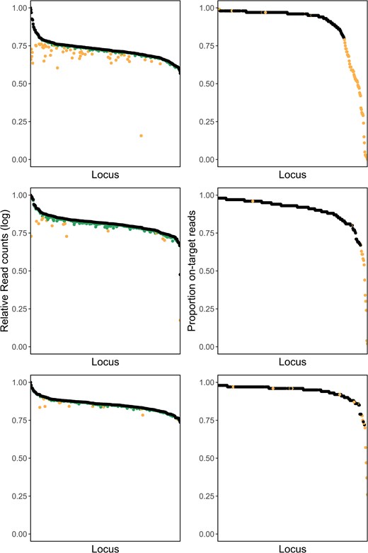
The left column is the relative log10 total read counts per locus (black) and relative log10 on-target read counts per locus (green, the darker color) of a GT-Seq panel for Striped Bass, showing the initial panel of 346 loci (top), panel of 279 loci after first optimization (middle), panel of 262 loci after second optimization (bottom). The right column is the proportion of on-target reads for each locus of a GT-Seq panel, showing the initial panel of 346 loci (top), panel of 279 loci after first optimization (middle), and panel of 262 loci after second optimization (bottom). Loci identified for culling during optimization steps are shown in orange (the lighter color).
Summary of initial GT-Seq optimization runs for Striped Bass. Rows include information on the number of primer pairs in each run, number of reads with intact i7 barcodes, number (percentage in parentheses) of reads with locus primer sequences, number (percentage in parentheses) of reads with target DNA sequence, and percent of total reads that correspond to the top 10% loci.
| Category | Round 1 | Round 2 | Round 3 |
|---|---|---|---|
| Number of primer pairs | 346 | 279 | 2,391 |
| i7 reads | 16,462,686 | 12,177,326 | 309,174,460 |
| i7 reads with primers | 15,240,894 (92.6%) | 10,334,621 (84.9%) | 288,493,849 (93.3%) |
| On-target reads | 9,613,337 (58.3%) | 8,972,963 (73.7%) | 269,207,774 (87.1%) |
| % reads in top 10% loci | 58.3% | 33% | 29.1% |
In the second round of optimization, the remaining 279 primer pairs were used to genotype 192 samples, producing 12,177,326 reads across all samples (Table 1). Of these, 84.9% contained valid primer sequences and 73.7% contained both primer sequence and target sequence. Sequence uniformity improved, with the top 10% of loci now contributing 33% of reads. When considering only the original 96 test samples, there were 5,676,837 total reads, of which 96.9% began with a primer and 90.1% were on target. The 96 samples extracted using Nexttec had lower values: of the 6,500,489 total reads, 74.3% matched primer probes and 59.3% were on target. Because this increase in primer dimers was not observed when negative controls were run with the same primers and plate-specific barcode, we could not exclude the dimers being an effect of the samples or extraction kit. We therefore excluded primers with forward primer on-target proportions less than 0.75 in plate 1 and less than 0.5 in plate 2. We also excluded two overamplifiers found in reverse reads on plate 2. Visual inspection of allele ratios of loci with contamination scores above 0.5 revealed no obvious issues, and so no primers were excluded. In total, 17 loci were removed from the panel in the second round of optimization (Figure 1).
In the final round of optimization, we assessed the performance of our panel on a full lane of 2,400 samples and sequenced a total of 309,174,460 reads (Table 1). Of these reads, 93.3% contained valid primer sequences and 87.1% contained both primer and target DNA sequence. The top 10% loci contributed 29.1% of all reads. We excluded 12 primers that had less than 70% on-target reads total in a particular extraction type, six primers that had visibly skewed heterozygote allele ratios, seven primers showing potential off-target amplification/paralogs, and one primer with very high amplification rates in samples extracted using Chelex. Genotype concordance comparisons identified five loci with discordant genotypes in multiple individuals. One of these five loci showed inconsistent amplification of one allele and was excluded. Four of the five loci were identified as having two SNPs in the target sequence. Two of these loci were retained after redesigning the probe to exclude the second SNP, while the other two were removed from the final panel. Primers and alleles for all four multi-SNP loci are included in the Supplementary Materials for use in future studies. In total, 29 loci were excluded from the final panel and our final SNP panel contained 233 loci. Genotype concordance of this 233-locus panel was high between GT-Seq and RAD-Seq: of 10,195 genotypes compared, 50 (0.5%) were discordant between the two methods.
Assignment accuracy of panels was assessed using leave-one-out and training-holdout methods of cross-validation in rubias, and a genetic clustering analysis was performed to compare performance of the final panel to the original RAD-Seq study. Assignment accuracy of panels did not change appreciably after each round of optimization and pruning. Using leave-one-out individual assignment on all four locus panels and a probability threshold of 0.8, assignment accuracy was 464/473 (98.1%) for panel 346, 455/473 (96.2%) for panel 279, 451/473 (95.3%) for panel 262, and 444/473 (93.9%) for panel 233. Of the 29 individuals not assigned back to their sampling region, 16 were assigned to a different sampling region (“misassigned”; Table S1 [see online Supplementary Material]) with high (>0.9) scaled likelihoods. We examined genetic clustering results for these individuals using our 233-locus panel as well as the original 1,278 SNPs to determine whether these individuals represented likely strays. The majority of individuals (14/16) showed admixed genotypes in the 233-SNP panel. Nine of these individuals were also highly admixed in the full 1,278-SNP data set, while four clearly clustered with the collection location (true misassignments) and three clustered with the region of assignment (likely strays). To minimize the effect of uneven sample sizes and eliminate high-grading bias in panel 233, we selected the same 239 individuals used to train the random forest model as a reference and the remaining 234 individuals as a holdout mixture. Scaled accuracy values were similar in training and holdout assignments (Figure 2). Assignment accuracy of holdout samples was 97.4% (Table 2), and of the five holdout samples misassigned in leave-one-out assignments, only one was still misassigned in this analysis, a “true” misassignment from Potomac River (Table 2).
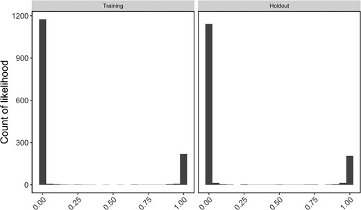
Histogram of scaled likelihoods for all reporting unit comparisons within the “training” and “holdout” data sets. Likelihoods are scaled from 0 to 1 for all reporting units to facilitate comparison, where 1 represents a high likelihood the individual is from a given reporting unit and 0 represents a low likelihood the individual is from the given reporting unit.
Assignment of 234 Striped Bass samples from six regions (proposed reporting groups) in rubias using 233 single nucleotide polymorphism (SNP) loci. Individuals were assigned using a reference set of 239 individuals used to select the SNP panel. Individuals were considered to belong to a reporting group if they were assigned with a confidence score of 80% or more. Rows correspond to the location individuals were collected in, while columns correspond to assigned reporting group. Abbreviations are as follows: GoSL = Gulf of St. Lawrence, SHUB = Shubenacadie River, WolSJR = Saint John/Wolastoq River, KEN-HUD = Kennebec River and Hudson River, DEL-CHPK = Delaware River and all rivers within Chesapeake Bay, and N. Carolina = Roanoke River and Cape Fear River. “Unknown” refers to the number of individuals assigned to a reporting unit with a posterior probability less than 80%.
| Region | GoSL | SHUB | WolSJR | KEN-HUD | DEL-CHPK | N. Carolina | Unknown |
|---|---|---|---|---|---|---|---|
| GoSL | 5 | 0 | 0 | 0 | 0 | 0 | 0 |
| SHUB | 0 | 2 | 0 | 0 | 0 | 0 | 0 |
| WolSJR | 0 | 0 | 1 | 0 | 0 | 0 | 0 |
| KEN-HUD | 0 | 0 | 0 | 21 | 0 | 0 | 0 |
| DEL-CHPK | 0 | 0 | 0 | 1 | 187 | 0 | 5 |
| N. Carolina | 0 | 0 | 0 | 0 | 0 | 12 | 0 |
Overall genetic structure found using the 233-SNP panel was similar to that found with 1,278-SNP panel. Clustering results using both sets of SNPs were similar (Figure 3; Figure 4 in LeBlanc et al., 2020). Pairwise FST trended slightly higher in the 233-SNP panel between reporting units, while relative levels of differentiation remained the same (Table 3). Pairwise FST was similar within reporting units; however, fewer rivers within Chesapeake Bay were significantly different from each other when 233 SNPs were used (Table S2).
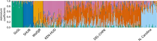
Individual admixture coefficients of Striped Bass in each of six reporting units assuming six genetic clusters (K), calculated using 233 single nucleotide polymorphism (SNPs). Individual Striped Bass are represented by vertical bars, with percent genotype similarity to each cluster represented by colors. Population shorthands are as follows: GoSL = Gulf of St. Lawrence, SHUB = Shubenacadie River, WolSJR = Saint John/Wolastoq River, KEN-HUD = Kennebec River and Hudson River, DEL-CHPK = Delaware River and all rivers within Chesapeake Bay, and N. Carolina = Roanoke River and Cape Fear River.
Average pairwise FST comparisons of Striped Bass samples among six reporting units using 233 SNP loci (below diagonal) compared with average pairwise FST using 1,278 SNPs (above diagonal). All pairwise FST values between reporting units were significant at p-value < 0.001. Abbreviations are as follows: GoSL = Gulf of St. Lawrence, SHUB = Shubenacadie River, WolSJR = Saint John/Wolastoq River, KEN-HUD = Kennebec River and Hudson River, DEL-CHPK = Delaware River and all rivers within Chesapeake Bay, and N. Carolina = Roanoke River and Cape Fear River. Astericks (*) are used as placeholders for cells that compare a population to itself.
| Region | GoSL | SHUB | WolSJR | KEN-HUD | DEL-CHPK | N. Carolina |
|---|---|---|---|---|---|---|
| GoSL | * | 0.201 | 0.179 | 0.183 | 0.185 | 0.190 |
| SHUB | 0.241 | * | 0.127 | 0.153 | 0.158 | 0.158 |
| WolSJR | 0.201 | 0.151 | * | 0.092 | 0.096 | 0.100 |
| KEN-HUD | 0.230 | 0.200 | 0.131 | * | 0.016 | 0.028 |
| DEL-CHPK | 0.237 | 0.210 | 0.134 | 0.025 | * | 0.026 |
| N. Carolina | 0.236 | 0.211 | 0.129 | 0.051 | 0.038 | * |
Using the final panel of 233 loci, rubias was used to create simulated mixtures of Striped Bass to test individual assignment performance in three scenarios. We performed a leave-one-out assignment to estimate the origin region of simulated individuals, allowing us to calculate the percentage of individuals in a mixture that were correctly assigned to a reporting unit. Mean assignment accuracies were high (99.9%) for all reporting units when all individuals in a mixture were from the same source (Figure 4, left panel). When simulated mixtures contained equal proportions of individuals from all six reporting units, overall accuracy was 98.6% (Figure 4, middle panel). Finally, we simulated mixtures containing large numbers of Chesapeake Bay individuals, a moderate number of Hudson Bay individuals, and small numbers of Roanoke River individuals. Assignment accuracy remained high for Chesapeake Bay and lower for Kennebec–Hudson River and North Carolina (mean accuracy 97.0%).
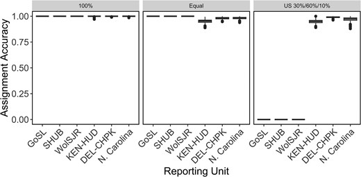
Box plots showing mean accuracy estimates from three simulation scenarios of six reporting units of Striped Bass across their native range, created using a data set of 233 SNPs. Scenarios are as follows: 100% simulations where all individuals in a mix are from the same region, a scenario where the mixture contains equal proportions of individuals from each region, and a scenario where the mixture contains 30% Hudson River, 60% Chesapeake Bay, and 10% Roanoke River individuals. Each scenario was run 1,000 times. Abbreviations are as follows: GoSL = Gulf of St. Lawrence, SHUB = Shubenacadie River, WolSJR = Saint John/Wolastoq River, KEN-HUD = Kennebec River and Hudson River, DEL-CHPK = Delaware River and all rivers within Chesapeake Bay, and N. Carolina = Roanoke River and Cape Fear River. For the box plots, the horizontal line in each box indicates the median, the box dimensions represent the 25th to 75th percentile ranges, whiskers show ranges up to 1.5 times the interquartile range from each hinge, and dots show all values outside of this range.
We also used both rubias and gsi_sim to simulate mixtures to examine the power of our panel to report the proportion of a stock’s fish from each of the six reporting regions, using the same three scenarios as in leave-one-out assignments (Figure 5). In the 100% scenario, mean percent error was less than 1% for all regions (0.4–0.6%). In simulated mixtures containing equal proportions of all six regions, error ranged from 0.006% to 0.4% (Figure 5). The proportion of Chesapeake Bay individuals was slightly overestimated (0.4%), while Kennebec–Hudson River and North Carolina proportions were slightly underestimated (0.2–0.4%). In mixtures containing only U.S. origin individuals, mean error was 1% above for Chesapeake Bay individuals, 0.9% under for Kennebec–Hudson River individuals, and 0.1% under for North Carolina individuals (Figure 5).

Box plots showing simulated and estimate mixing proportions from three simulation scenarios of six reporting units of Striped Bass across their native range, created using a data set of 233 SNPs. Scenarios are as follows: 100% simulations where all individuals in a mix are from the same region, a scenario where the mixture contains equal proportions of individuals from each region, and a scenario where the mixture contains 30% Hudson River, 60% Chesapeake Bay, and 10% Roanoke River individuals. Simulations in the top row were run in rubias using the full data set to create simulated genotypes, while the bottom row shows simulations created in gsi_sim where simulated genotypes were created using holdout individuals and were matched to regions using training individuals as a reference. Each scenario was run 1,000 times. Abbreviations are as follows: GoSL = Gulf of St. Lawrence, SHUB = Shubenacadie River, WolSJR = Saint John/Wolastoq River, KEN-HUD = Kennebec River and Hudson River, DEL-CHPK = Delaware River and all rivers within Chesapeake Bay, and N. Carolina = Roanoke River and Cape Fear River. For the box plots, the horizontal line in each box indicates the median, the box dimensions represent the 25th to 75th percentile ranges, whiskers show ranges up to 1.5 times the interquartile range from each hinge, and dots show all values outside of this range.
DISCUSSION
Mixed stocks of fish, such as those seen in Striped Bass, present a challenge for fisheries managers seeking to regulate fishing pressure to maintain stable stocks over time (Hilborn, 1985). Attempts to resolve mixed Striped Bass stocks with fish originating from U.S. populations using genetic markers have long been hampered by low genetic differentiation (Gauthier et al., 2013) and high variation in stock composition from year to year (Wirgin et al., 1997). Here we present a panel of 233 SNP markers able to assign Striped Bass to six reporting units along its migratory range, including the three major reporting units known to contribute migrants to coastal stocks in the United States. Our panel represents an improvement over previous targeted mixed-stock analysis markers in its ability to differentiate between all three U.S. reporting units with high (>95%) accuracy. A microsatellite panel developed by Gauthier et al. (2013) was able to assign 52% of known-origin Striped Bass to their sampling location in Hudson River, Delaware–Chesapeake Bay, Roanoke River, or the Santee–Cooper river system. Fisheries management in this region has historically used mixed-stock analysis only to differentiate between Hudson River and Chesapeake Bay reporting units due to the difficulty in developing a genetic panel able to identify Striped Bass from Roanoke River, North Carolina, and the historically low number of Roanoke River Striped Bass in coastal mixed stocks (ASMFC, 2022b).
Simulations and assignments of known individuals show overall high accuracy in assignment and low error in mixture estimates. We saw higher levels of misassignment when leave-one-out assignment was performed on all individuals versus when training individuals were used as a reference, likely due to the large number of Delaware–Chesapeake Bay individuals (n = 248) relative to other reporting units (n = 32–71). We confirmed that some, but not most, misassignments were due to straying between Kennebec–Hudson River and Delaware–Chesapeake Bay—behavior that has previously been documented in acoustic telemetry studies (Secor et al., 2020a). Additionally, four juveniles were admixed between Saint John/Wolastoq River and Chesapeake Bay, two highly divergent reporting units (Table 3). All four were assigned to Delaware–Chesapeake Bay with high likelihood, in both the 233-locus panel and the original RAD-Seq study (LeBlanc et al., 2020). When this kind of admixture may be present in a study it is recommended to perform analyses that do not specify a priori sampling units, such as genetic clustering or principal component analysis. However, simulations indicate that broadscale mixed-stock analysis will not be significantly biased by this type of misassignment of admixed individuals.
Characterization of Striped Bass migration patterns and stock mixtures has been ongoing for almost a century, and many techniques have been employed to this end (ASMFC, 2022c; Chapoton & Sykes, 1961; Waldman et al., 1988). Conventional physical tagging studies, the most basic tool, are typically hindered by lack of information about a fish’s origin and very low rates of recapture (<5%), necessitating a great number of tags and substantial tagging effort. In the past several decades, acoustic tagging studies have successfully characterized specific migration routes along the coast (Andrews et al., 2018; Carmichael et al., 1998; Secor et al., 2020b), and the utility of this technology is continually improving as researchers add to arrays and cooperative data sharing networks, such as the Ocean Tracking Network and the Mid-Atlantic Acoustic Telemetry Observation system. However, the costs for a large-scale study requiring data from thousands of fish are prohibitively high because individual acoustic tags cost more than Can$400 (US$300), making their use for comprehensive determination of mixed-stock harvest infeasible. Genetic markers such as mitochondrial fragments and microsatellites were able to detect broadscale differences between regions at lower confidence levels (Brown et al., 2005; Gauthier et al., 2013; Wirgin et al., 1997), while more powerful SNPs have recently been used to discriminate among smaller geographic regions or even individual rivers (LeBlanc et al., 2020; Wojtusik et al., 2022). Therefore, genetic markers provide a possible alternative. The GT-Seq panels, like the one developed here, are ideal for studies where the focus is on maximizing the number of individuals being genotyped and minimizing the laboratory and computational resources required to collect and process data. While RAD-Seq methods, including Rapture, can achieve greater resolution among populations, these techniques are more difficult to implement on a large scale in a cost-effective way, and the bioinformatics processing of data has a steep learning curve (McKinney et al., 2022; Meek & Larson, 2019). The cost for consumables and sequencing for a full GT-Seq library of 2,400 samples was Can$6/sample (US$4.40). For a half library of 1,200 samples, the price increased to about $7/sample (US$5.14) and continued to increase to $15/sample (US$11) for 196 samples and $25/sample (US$18.34) for 96 samples. In comparison, a RAD-seq panel constructed in our lab using current sequencing technologies is estimated to cost $30/sample for 96 (US$22), $18/sample for 192 (US$13), and between $13 and $18 per sample for all amounts greater than 192 (US$9–13). Our method, therefore, becomes more cost-efficient than RAD-Seq-based targeted sequencing methods when more than 200 individuals need to be genotyped. Once genotyped, downstream bioinformatics can be performed on an office desktop computer with no need for high performance computing servers, all while achieving high levels of accuracy (>90%) for all reporting units.
In the present study, we focused on optimizing a small SNP panel with the aim of allowing room for the addition of more SNPS, improving power while retaining the accessibility of GT-Seq. Simulations using known-origin individuals indicate a high degree of accuracy, and moving forward further simulation work can be done to help guide coastwide sampling programs for stock assessment and to assess if empirical results mirror simulation findings. A number of avenues are available that may allow for improvement in the future, such as an improved reference data set that allows for the incorporation of microhaplotypes (Baetscher et al., 2018) identified in this study. Microhaplotypes have been shown to increase the power of GT-Seq panels (McKinney et al., 2017). Additionally, a recent RAD-Seq study discovered 1,300 SNPs that were able to discriminate among Striped Bass from individual rivers within the Chesapeake Bay (Wojtusik et al., 2022), and these SNPs could be investigated to identify potential loci suitable for inclusion in our GT-Seq panel. The process of adding new markers to a GT-Seq panel is relatively straightforward and should not require multiple rounds of testing if the number of new markers is small. We expect that the SNP panel developed in this paper therefore will be an important genetic tool for long-term monitoring and management of Striped Bass even as new genetic markers are discovered in the future.
SUPPLEMENTARY MATERIAL
Supplementary material is available at Transactions of the American Fisheries Society online.
DATA AVAILABILITY
Full primer sequences for the 233-SNP panel are available in the Supplementary Materials, as well as reference samples in genepop format.
ETHICS STATEMENT
Newly collected tissue in this study was collected by Massachusetts Division of Marine Fisheries and processed at University of Massachusetts Amherst, all under Institutional Animal Care and Use Committee Protocol 2015-0012, through the University of Massachusetts Amherst.
FUNDING
We would like to express our gratitude to the Massachusetts Division of Marine Fisheries, the Natural Sciences and Engineering Research Council of Canada, Canada Research Chairs, ResearchNB, and the University of New Brunswick for financial and administrative support. Funding was also provided by Atlantic Coastal Cooperative Statistics Program Grant NA21NMF4740481, “Creation of a Genetic Stock Identification program for Atlantic coast Striped Bass (Morone saxatilis).”
ACKNOWLEDGMENTS
Genome Quebec and Azenta Life Sciences provided sequencing and demultiplex services for this project. We would also like to thank those involved in fieldwork and collection of the tissue samples used in this study. Paul Bentzen provided tissue samples from Miramichi River Striped Bass in Bras d'Or Lake. Samuel Andrews, with help from Scott Young and Keith Young, provided Striped Bass from the Saint John/Wolastoq River, New Brunswick. The Striped Bass Research Team coordinated sampling from the Shubenacadie River, with help from local anglers. Beth Versak (Maryland Department of Natural Resources) coordinated sampling from the Chesapeake Bay, Andy Kahnle (New York State Department of Environmental Conservation Bureau of Marine Resources, Hudson River Fisheries Unit) and Matt Fisher (Delaware Department of Natural Resources and Environmental Control, Division of Fish and Wildlife) coordinated sampling from the Hudson River. Coordination of the collection of Kennebec River juveniles was done by Gail Wippelhauser and Jason Bartlett from the Maine Department of Marine Resources. Jeremy McCargo, as well as the North Carolina Division of Marine Fisheries, and Jeff Evans and Kevin Dockendorf (North Carolina Wildlife Resources Commission), collected Roanoke River and Cape Fear River samples. Coastal Massachusetts samples were collected by the Massachusetts Division of Marine Fisheries. Finally, several lab technicians helped to perform DNA extraction and PCR amplification of the samples used in this study, including Melissa Morrison, Laken Devost, and Marijune Tiamzon.
REFERENCES
Author notes
CONFLICTS OF INTEREST: The authors declare that there is no conflict of interest.
