Pauli–Villars Regularization of Kaluza–Klein Casimir Energy with Lorentz Symmetry

Abstract

1. Introduction

The Casimir effect is a macroscopic quantum effect that has been observed in various experiments and the observed values are in good agreement with theoretical predictions [1–5]. The Casimir energy is defined as the energy difference between the vacuum energy in a compact space, such as a space enclosed by conducting plates, and that in a noncompact space. The vacuum energy in quantum field theory (QFT) is generally divergent and must be regularized, such as the cutoff regularization, in which the cutoff scale Λ_cut is set for the momenta of virtual particles in the loops. It is well known that the Casimir energy remains finite even in the limit of Λ_cut → ∞. The scale Λ_cut is regarded as a scale at which the theory under consideration breaks down and is replaced with a more fundamental theory. The Casimir effect also plays an important role in extra-dimensional models. The quantum correction for the extra-dimensional models is Kaluza–Klein (KK) Casimir energy, which depends on the compactification scale m_KK and determines the physical properties of the extra-dimensional models [6–9]. Since the extra-dimensional models are nonrenormalizable, they should be regarded as effective theories of more fundamental ones, such as string theory or quantum gravity (QG). Hence Λ_cut cannot be infinite, and may be close to m_KK. In the latter case, the unknown ultraviolet (UV) physics can affect the KK Casimir energy. This indicates that the Casimir energy in the extra-dimensional models have regularization dependence [10–15], in contrast to the case of renormalizable theories, in which we can safely take the limit Λ_cut → ∞. In particular, one of the authors suggests that the Casimir energy receives a large correction from the UV physics when Λ_cut is not far from m_KK in the cutoff regularization scheme [15].

In 3 + 1D QFT, there is a significant discussion regarding Lorentz symmetry violation in the regularization of vacuum energy. Indeed, when utilizing the cutoff regularization, the UV divergences break the Lorentz symmetry [16–18]. If this Lorentz symmetry violation is considered as an actual physical phenomenon, it could lead to significant cosmological issues [19]. When we consider the Friedmann–Lemaître–Robertson–Walker (FLRW) universe with the metric ds² = dt² − a²(t)δ_ijdxⁱdx^j, the semiclassical Friedmann equations for a flat universe with a vacuum state are given by

where Λ_cc is the cosmological constant, the hat denotes an operator, |$\hat{\rho }$| is the energy density, |$\hat{p}$| is the pressure, the dot denotes the time derivative, and |$H\equiv \dot{a}/a$| is the Hubble parameter. A combination of these equations leads to

In the cutoff regularization, we have

where δ_if is the Kronecker delta with i = b, f for bosons and fermions respectively, and m is the mass. This shows that the UV divergences directly contribute to the dynamics of the universe.¹ On the other hand, we should note that Eq. (4) for the fermionic contribution clearly violates the null energy condition (NEC). The NEC is known as a necessary condition to eliminate any pathological space-time or unphysical geometry [21,22] and it states that T_μνn^μn^ν ≥ 0 for any null light-like vector n^μ. This is summarized as ρ + p ≥ 0 for the FLRW metric. In the context of the vacuum energy of the quantum fields and its regularization, there exist issues related to the breaking of Lorentz symmetry and the violation of the NEC.

In this paper, we explore the KK Casimir energy density and pressure from compact dimension. We particularly study the UV sensitivity of the KK Casimir energy. As we will show in the next section, the analytic regularization inherently omits the UV contributions, and the cutoff regularization violates the Lorentz symmetry in the vacuum state. Therefore, we adopt the Pauli–Villars regularization, which effectively demonstrates the cancellation of large quantum corrections by the contributions of high-energy virtual particles in the effective field theory. We further specify the necessary conditions on the regulator fields to preserve Lorentz symmetry.² Although spontaneously broken supersymmetric (SUSY) models satisfy some of these conditions, SUSY is not enough to ensure the Lorentz invariance of the vacuum state.

The rest of this paper is organized as follows. In Section 2, we review the analytic and cutoff regularizations of the KK Casimir energy density and pressure. We point out that these regularizations are not adequate to evaluate the UV sensitivity of the Casimir energy preserving the Lorentz symmetry. In Section 3, we consider the Pauli–Villars regularization to regularize the Casimir energy density, and provide the necessary conditions for regulator fields to preserve Lorentz symmetry. In Section 4, we numerically calculate the Casimir energy density and pressure in the Pauli–Villars regularization, and evaluate their dependence on the UV regulator mass scale. In Section 5, we conclude our work.

2. Regularizations

We take the following semiclassical treatment [24], which approximately combines QFT and general relativity (GR), and is expected to be reliable under conditions where QG is not important. We treat space-time classically and use the expected value of the quantized stress–energy tensor in Einstein’s equations. Hence, the quantum effect of matter fields on space-time geometry can be approximately described by the semiclassical equations³

where G_μν is the Einstein tensor, Λ_cc is the cosmological constant, and 〈T_μν〉 is the expected value of the quantum stress–energy tensor. Phenomenologically, such treatment will suffice.⁴

It is known that the (quantum) vacuum is Lorentz invariant to a high accuracy from observations [38,39]. Therefore, the vacuum energy density |$\hat{\rho }$| must give rise to an energy–momentum tensor in the 4D Minkowski space-time of the form

where |$\eta _{\mu \nu }={\rm diag}\, (-1,1,1,1)$| is the Minkowski metric, and thus the quantum correction to the vacuum energy density is renormalized by the cosmological constant Λ_cc. Note that Eq. (7) indicates that

where |$\hat{p}\equiv T^{\rm vac}_{11}=T^{\rm vac}_{22}=T^{\rm vac}_{33}$| is the vacuum pressure. Therefore, the LHS of Eq. (8) measures the violation of the Lorentz symmetry.

2.1. Formal expressions for energy density and pressure

To simplify the discussion, we consider a real scalar theory in a flat 5D space-time, and one of the spatial dimensions is compactified on S¹/Z₂:

where μ = 0, 1, ⋅⋅⋅, 4, and M_bulk is a bulk mass parameter. The coordinate of the compact dimension is denoted as y ≡ x⁴. The fundamental region of S¹/Z₂ is chosen as 0 ≤ y ≤ πR, where R is the radius of S¹. The real scalar field Φ is assumed to be Z₂ odd. Then the KK masses are given by

The vacuum energy density and the vacuum pressure in the 4D effective theory are formally expressed as

These obviously diverge, and we need to regularize them. In the following, we review the analytic and the momentum-cutoff regularizations, and mention unsatisfactory points for our purpose. To make the relation between them clear, we introduce the cutoff for the KK mode number N_cut, the momentum cutoff Λ_cut, and the complexified dimension d. Then, Eq. (11) is regularized as

where μ is some scale to adjust the mass dimension. Naively, the cutoff scales for the 3D momentum and the fifth one are expected to be common. Thus we assume that |$m_{N_{\rm cut}}\simeq \Lambda _{\rm cut}$|⁠, or more specifically

Performing the |$\vec{k}$|-integral, we obtain

where Γ(α) is the Euler gamma function, B_z(α, β) is the incomplete beta function, and

2.2. Analytic regularization

2.2.1. Review of conventional derivation

The most popular regularization scheme for the calculation of the Casimir energy is the combination of the dimensional regularization and the zeta-function regularization, which we call analytic regularization in this paper.

Let us take the limit Λ_cut → ∞, i.e. ϵ_n → 0, keeping d − 3 nonzero, in Eq. (14). Then, the incomplete beta function reduces the complete beta function, and becomes n-independent:

Thus, Eq. (14) becomes

The infinite sum over the KK modes is evaluated by the zeta-function regularization technique [8,40,41]. Using the formula (B10) with Eq. (B11) in Appendix  B, the energy density is expressed as

where |$\bar{M}_{\rm bulk}\equiv RM_{\rm bulk}$|⁠, and K_α(z) is the modified Bessel function of the second kind. The first term diverges as d → 3, but it does not depend on R and is irrelevant to the stabilization of the extra dimension. Thus we simply neglect it. We require that the vacuum energy density in the decompactified limit R → ∞ vanishes [42]. Thus the Casimir energy density, which is a function of R, is defined as

Note that the subtraction should be performed for the 5D energy density since the second term is the quantity in the decompactified limit. Then, the second term in Eq. (18) is canceled, and we obtain

We have taken the limit d → 3 at the last step. Similarly, the vacuum pressure is calculated as

In the massless case M_bulk = 0, Eq. (20) reduces to the well known form

where ζ(s) is the Riemann zeta function.

From Eqs. (20) and (21), we can see that the sum of the KK Casimir energy density and pressure are exactly zero:

Thus, the Lorentz symmetry and NEC are both preserved in this regularization.⁵

2.2.2. Cutoff sensitivity in analytic regularization

Although the formulae (20) or (21) are useful because of their rapid convergent property, the analytic continuation processes make it difficult to see how the divergent terms are removed. It is well known that this regularization only captures the logarithmic divergences, and is insensitive to the power-law divergences of Λ_cut. To see the situation, let us review the procedure that we have performed in Eq. (16) in more detail. As long as Λ_cut is kept finite, the incomplete beta functions in Eq. (14) are well defined for any values of the dimension d. Before taking the limit Λ_cut → ∞, let us consider a case that d < −1. Then, using Eq. (A6) in Appendix  A, the incomplete beta functions are expanded as

Since all the powers on the RHS are positive for d < −1, we can safely take the limit Λ_cut → ∞ (i.e. ϵ_n → 0), and drop all ϵ_n-dependent terms. After dropping them, we can move d to a value close to 3. This is what we have done in Eq. (16). However, if we keep the ϵ_n-dependent terms when we move d to a value close to 3, the second and third terms on the RHS of Eq. (24) have negative powers, and correspond to the quartic and quadratic divergences, respectively.⁶ Therefore, what we have done in Eq. (16) is just to drop the quartic and quadratic divergent terms by hand.

A similar prescription has been performed when we apply the zeta-function regularization for the infinite sum over the KK modes. If we keep the cutoff Λ_cut finite, the incomplete functions in Eq. (14) depend on the KK level n, and cannot be factored out from the summation over n. Therefore, it is not easy to perform the exact calculation of Eq. (14). Hence we investigate the following expression instead:

where a ≡ 1/N_cut is a tiny positive constant. Instead of the sharp cutoff at n = N_cut, we introduce the damping factor |$e^{-a^2n^2}$|⁠, which suppresses the contribution of heavy KK modes with m_n > Λ_cut.⁷ Then, Eq. (25) is rewritten as

where U(α, β; M²) is defined in Eq. (B1) in Appendix  B. According to Eq. (B3) with Eqs. (B4) and (B12), this has the following terms:

where C_i(β; M²) (i = 1, 2, 3) are defined in Eq. (B13), and

and the ellipsis denotes terms that appeared in Eq. (18) and irrelevant terms that will vanish in the limit of Λ_cut → ∞ when d = 3. In the limit of d → 3 keeping Λ_cut finite, the terms shown in Eq. (27) represent power-law-divergent terms up to quintic in Λ_cut. This is expected because we are considering the 5D theory. In the derivation of Eq. (18), we have taken the limit of Λ_cut → ∞ for d < −2, where all terms shown in Eq. (27) vanish. However, this treatment is equivalent to just dropping those terms by hand. Therefore, the analytic regularization is inappropriate for studying the UV sensitivity of the Casimir energy density or pressure.

2.3. Cutoff regularization

Next, we consider the cutoff regularization. Take the limit d → 3, keeping Λ_cut finite, in Eq. (14). Then we obtain

The sum of the vacuum energy density and pressure is

where the logarithmic terms exactly cancel but the cutoff divergences remain. Namely, the Lorentz symmetry is violated in this regularization. If Φ is replaced with a 5D fermion, an overall minus sign appears in the above expressions. Hence NEC is also violated in that case.

For a light mode with m_n ≪ Λ_cut, its contribution to the vacuum energy and the vacuum pressure can be expanded as

After summing over the KK modes, the leading terms of |$\left\langle {0}\,\vert \,{\hat{\rho }}\,\vert \,{0}\right\rangle$| and |$\left\langle {0}\,\vert \,{\hat{p}}\,\vert \,{0}\right\rangle$| are

where N_cut is defined in Eq. (13). Since these are proportional to R, they are canceled in the Casimir energy density and pressure defined in Eqs. (19) and (21), respectively. However, the other terms remain and violate the Lorentz symmetry. Thus the cutoff regularization is considered to be problematic for the calculation of the Casimir energy [16–18].

From the physical point of view, contributions of massive KK modes near the cutoff scale Λ_cut should be suppressed by UV physics. In the previous work [15], we introduced a damping function, such as

or

where A ≳ 10 is a positive constant that controls the steepness around the cutoff scale, and inserted it into Eq. (14) as

Then we obtain a finite value for the Casimir energy density, which agrees with the value obtained by Eq. (21).⁸ The cutoff regularization considered in this subsection corresponds to the limit of A → ∞ in Eq. (34). It is known that the regularization with such a sharp cutoff provides a divergent Casimir energy density, and should not be applied to the calculations for the Casimir energy density and pressure [15].

3. Pauli–Villars regularization

As mentioned in Section 2.3, the contributions of massive KK modes near Λ_cut should be suppressed by the UV physics, such as contributions of new particles with masses of |${\cal O}(\Lambda _{\rm cut})$|⁠. Such contributions can be mimicked by the Pauli–Villars regulators. However, a single regulator that has opposite statistics and a large mass M_reg is not enough to suppress contributions of KK modes heavier than M_reg.⁹ Hence, for each KK mode with mass m_n, we introduce k species of regulators. Then, its contributions to the Casimir energy density and pressure are modified as

where |$\tilde{\rho }$| and |$\tilde{p}$| are defined in Eq. (31) and M_i and an integer c_i denote the mass and the degree of freedom for the ith regulator, respectively. We assume that all M_i (i = 1, 2, ⋅⋅⋅, k) are of |${\cal O}(M_{\rm reg})$|⁠. Note that we introduce both bosonic (c_i < 0) and fermionic (c_i > 0) regulators. Then, using the expanded expressions in Eq. (31), we have

If we require the integers c_i (i = 1, 2, ⋅⋅⋅, k) to satisfy [17,23]¹⁰

the Lorentz-violating terms are canceled, and we obtain

in the limit of Λ_cut → ∞. Hence we have

The first condition in Eq. (38) is the requirement of the balance between the bosonic and fermionic degrees of freedom. The second one has the same form as the supertrace mass formula in a model that has spontaneously broken supersymmetry (SUSY) [43]. Namely, the first two conditions in Eq. (38) are automatically satisfied in such a model. To preserve the Lorentz symmetry, however, the third condition is also necessary. It is intriguing to discuss the possibility of constructing a SUSY model in which all conditions in Eq. (38) are satisfied [23].

To suppress the contributions of massive KK modes heavier than M_reg, we should also require that

This is rewritten as

In the case of

we can solve Eq. (38), and obtain

For c₂ = 3, we have four bosonic and four fermionic degrees of freedom in total that can be embedded into a chiral multiplet in a (spontaneously broken) SUSY model. In the following, we consider the case of Eq. (43) with c₂ = 3 as a specific example.

We assume that |$M_i^2$| (i = 1, 2, 3) are functions of |$m_n^2$| and |$M_{\rm reg}^2$|⁠. In solving Eq. (42), we are interested in the KK modes with m_n ≫ M_reg. Thus, we expand |$M_1^2$| as

where |$\delta \equiv M_{\rm reg}^2/m_n^2$|⁠. Using this expression and Eq. (44), we can expand the LHS of Eq. (42) as

where the coefficients |${\cal C}_i$| (i = 1, 2, ⋅⋅⋅, 6) are functions of α, β₁, and β₂. The requirement (42) indicates that all |${\cal C}_i$| (i = 1, 2, ⋅⋅⋅, 6) vanish. We find that |${\cal C}_1$|⁠, |${\cal C}_2$|⁠, and |${\cal C}_3$| automatically vanish, and do not give any constraints on α, β₁, and β₂. The coefficient |${\cal C}_4$| is a function of only α,

and the solution of |${\cal C}_4=0$| is α = 1. Under the condition α = 1, we can easily see that both |${\cal C}_5$| and |${\cal C}_6$| vanish identically. Therefore, we can take β₂ = 0, and assume that

as a solution to Eq. (42). If we rescale |$M_{\rm reg}^2$|⁠, we can always set β₁ = 1. As a result, we can choose a solution of Eq. (42) (and Eq. (38)) as

This result indicates that the regulators can be regarded as the KK modes for 5D bulk fields. In fact, if we introduce one fermionic 5D field with the (squared) bulk mass |$M_{\rm bulk}^2+M_{\rm reg}^2$|⁠, three fermionic 5D fields with |$M_{\rm bulk}^2+\frac{1}{3}M_{\rm reg}^2$|⁠, and three bosonic 5D fields with |$M_{\rm bulk}^2+\frac{2}{3}M_{\rm reg}^2$|⁠, the conditions (38) and (41) are satisfied for each KK mode.

Before ending this section, we comment on the relation to analytic regularization. In that regularization, ρ_n and p_n are read off from Eq. (17) as

where γ_E is the Euler–Mascheroni constant. We have used Eq. (A3) at the last equality. After the minimal subtraction, we have

To match Eq. (37) with this result, a further additional condition has to be imposed [17]:

Therefore, the number of regulator species has to be chosen as k ≥ 4. Then, Eq. (37) agrees with Eq. (51) in the limit of Λ_cut → ∞. However, we do not have a simple solution for Eq. (38) when k ≥ 4. For example, if we assume that k = 4 and c₃ = −c₄, we obtain from Eq. (38)

where

Plugging this into Eq. (52) and solving it, we can express |$M_2^2$| in terms of |$M_1^2$| in principle. As a result, |$M_i^2$| (i = 2, 3, 4) can be expressed as functions of |$M_1^2$| and |$m_n^2$|⁠. However, we do not have analytic expressions for them in general.

As we will see in the next section, even if the condition (52) is not imposed, the result agrees well with the one obtained in the analytic regularization (20) as long as |${\rm min}\, (M_1^2,M_2^2,M_3^2)\gt m_{\rm KK}\equiv R^{-1}$|⁠.

4. Regulator mass dependence of Casimir energy

In this section, we will numerically calculate the Casimir energy density and pressure in the Pauli–Villars regularization, and evaluate their dependence on the regulator mass scale M_reg. As a specific example, we choose the regulator masses as Eq. (49). In this case, the energy density and pressure for the vacuum are expressed as

where a ≡ (M_regR)⁻¹, and

Figure 1 shows the profile of the function F(x) for various values of |$\hat{M}_{\rm bulk}$|⁠. We can see that the contribution of the KK modes damps around x = 1, which corresponds to the regulator mass scale M_reg.

Fig. 1.

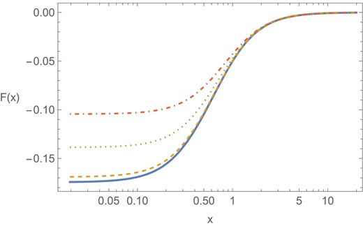
The profile of the function F(x) defined in Eq. (56). The bulk mass is chosen as |$\hat{M}_{\rm bulk}=0$| (solid), 0.1 (dashed), 0.3 (dotted), and 0.5 (dot–dashed) from bottom to top.

Open in new tabDownload slide

According to Eq. (19), the Casimir energy and pressure are given by

where¹¹

In order to evaluate Δ(a), the Euler–Maclaurin formula is useful [44–46]. Then we obtain

where B_2p are the Bernoulli numbers, q is an integer greater than 1, and

with the Bernoulli polynomial B_q(x). At the last step in Eq. (60), we have used that

Here we set q = 2. Then, noting that F⁽¹⁾(0) = 0 from Eq. (C1), Eq. (60) becomes

where the explicit form of F⁽²⁾(x) is shown in Eq. (C1) in Appendix  C, and

To see the deviation of the Casimir energy (57) from the one obtained in the analytic regularization (20), we define

where |$\left\langle {0}\,\vert \,{\hat{\rho }}\,\vert \,{0}\right\rangle _{\rm Casimir}^{\rm anal}$| denotes Eq. (20). Figure 2 shows the ratio r_cas as a function of a = m_KK/M_reg, where m_KK ≡ 1/R is the KK mass scale. We can see that the result obtained by the Pauli–Villars regularization agrees well with that of the analytic regularization as long as the compactification scale m_KK is well below the regulator mass scale M_reg.

Fig. 2.

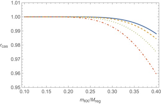
The ratio r_cas defined in Eq. (65) as a function of m_KK/M_reg. The bulk mass is chosen as M_bulk/M_reg = 0 (solid), 0.1 (dashed), 0.2 (dotted), and 0.3 (dot–dashed), respectively.

Open in new tabDownload slide

Before ending the section, one comment is in order. The above results can also be expressed by using the analytic regularized formula (20). As mentioned below Eq. (49), the current choice of the Pauli–Villars regulators can be understood as 5D fields. Thus, the Casimir energy density in Eq. (55) is also expressed as

where

Thus, Eq. (65) can be rewritten as

where |$\bar{M}_{\rm bulk}=RM_{\rm bulk}$|⁠, |$\bar{M}_{\rm reg}=RM_{\rm reg}$|⁠, and

The function |$\Delta (\bar{M}_1,\bar{M}_2)$| is exponentially suppressed when |$\bar{M}_1\ll \bar{M}_2$|⁠, but becomes nonnegligible when |$\bar{M}_2={\cal O}(\bar{M}_1)$|⁠. Since the infinite summation in Eqs. (67) or (69) converges much faster than the KK summation, this expression is convenient to the numerical computation.

5. Discussions and conclusions

We have studied the dependence of the Casimir energy density on the UV dynamics in the context of a 5D model with a compact dimension. In contrast to renormalizable theories, a nonrenormalizable theory, such as our 5D model, should be regarded as an effective theory, and be replaced by a more fundamental theory at some high energy scale M_UV. A typical situation is that some new particles appear at a scale around M_UV, and cancel quantum corrections from the light fields in the 5D effective theory.

If M_UV is not far from m_KK, the existence of the new particles can affect low-energy observables, such as the Casimir energy density. We have evaluated such effects on the Casimir energy density (and pressure). The most popular way of calculating the Casimir energy is the method using analytic regularization because the resultant expression is convenient for the numerical evaluation and the regularization preserves various symmetries, including the Lorentz symmetry. However, this regularization removes the power-law divergences by hand, and thus is inappropriate for our purpose, as we showed in Section 2.2.2. Instead of this, we work in the Pauli–Villars regularization, which mimics the situation that new particles cancel the quantum corrections from the light particles. To preserve the Lorentz symmetry of the vacuum, we have to prepare more than one regulator for each mode, and their masses and the degrees of freedom have to satisfy some conditions (see Eqs. (38) and (41)). It should be noticed that two of them are automatically satisfied in a (spontaneously broken) SUSY model. The result in Eq. (49) indicates that the Pauli–Villars regulators can be regarded as the KK modes for 5D bulk fields. In the case that the model is embedded into a (spontaneously broken) SUSY 5D theory, the scalar field Φ and the bulk regulators should be embedded into a 5D SUSY multiplet. Thus, the example of the regulators considered in Section 3 must be modified. Needless to say, the deviation from the result in the analytic regularization depends on the choice of Pauli–Villars regulators. Still, our example shows a typical order of magnitude for the deviation.

If we do not impose the condition (52), it is not guaranteed that the resultant Casimir energy density (or pressure) will agree with that obtained by analytic regularization. We numerically evaluate them and confirm that they agree well with each other even if Eq. (52) is not satisfied, as loong as the KK mass m_KK and the bulk mass M_bulk are smaller than all the regulator masses.

Acknowledgement

H.M. would like to thank Yoshio Matsumoto for useful comments and for checking our manuscripts in the early stages. The work of H.M. was supported by JSPS KAKENHI Grant No. JP22KJ1782 and No. JP23K13100.

Funding

Open Access funding: SCOAP³.

A. Complete and incomplete beta and gamma functions

A.1. Definitions and properties

The integral expressions of the complete beta and gamma functions are given by

which are valid only for |${\rm Re}\, \alpha \gt 0$| and |${\rm Re}\, \beta \gt 0$|⁠. They are related as

This relation holds over the whole domain of the beta function. The gamma function behaves near α = 0, −1, −2 as

where γ_E is the Euler–Mascheroni constant.

The incomplete beta functions are defined as

for |${\rm Re}\, \alpha \gt 0$|⁠, and the upper and lower incomplete gamma functions are defined as

where the integral expression of γ_z(α) is valid only for |${\rm Re}\, \alpha \gt 0$|⁠. From Eq. (A4), we obtain

for |${\rm Re}\, \alpha \gt 0$| and |${\rm Re}\, \beta \gt 0$|⁠.

Similarly, the incomplete gamma function can be expanded as

The incomplete beta function is also expanded as

We can show this by differentiating both sides concerning ϵ, and checking that they coincide. For β > 0, Eq. (A8) reduces to Eq. (A2) in the limit of ϵ → 0.

A.2. Explicit forms

Here we show the explicit forms of the incomplete beta functions that appear in Section 2.3:

Since

where X ≡ Λ_cut/m_n, the above functions can be expressed in the form of

when |${\rm Re}\, \alpha \gt 0$|⁠. By differentiating this concerning X, we have

Since |$B_{\frac{X^2}{X^2+1}}(\alpha ,\beta )|_{X=0}=0$|⁠, Eq. (A11) is reexpressed as

From this expression, we obtain

B. Formulae for zeta-function regularization

In order to evaluate the regularized sums in Eq. (14), we define

where a is a tiny positive constant, and

Using the formula (A8), this is expressed as

where

Here note that S_δ(β; M²) can be rewritten as

where |$\vartheta (t)\equiv \sum _{n=1}^\infty e^{-n^2t}$| is the Jacobi theta function, which has the property

Using this property of ϑ(t) and the definition of the gamma function, |$S_{a^2x}(\beta ;M^2)$| is expanded as

where the constants c_j are defined by

and the function H_b(z) is defined as

When |${\rm Re}\, \beta \gt \frac{1}{2}$|⁠, all the powers of a are positive, and we can take the limit of a → 0 and obtain

When |${\rm Re}\, \beta \lt 1$|⁠, the integral in the last term is expressed as

Substituting Eq. (B7) into the first expression in Eq. (B4), we obtain

where

C. Derivatives of F(x)

Here we collect the explicit forms of derivatives of F(x) defined in Eq. (56):

For x ≫ 1, F⁽²⁾(x) is expanded as

Footnotes

References