Convergence of Ginzburg–Landau Expansions: Superconductivity in the Bardeen–Cooper–Schrieffer Theory and Chiral Symmetry Breaking in the Nambu–Jona-Lasinio Model

Abstract

1. Introduction

Power series expansions are ubiquitous in physics. Some examples can be found in the perturbative expansions appearing throughout quantum mechanics and quantum field theory (QFT). Another example is the paradigm of effective field theories (EFT), based on a systematic expansion at certain scales. Hydrodynamics, for instance, is an EFT based on a gradient expansion. Ginzburg–Landau (GL) theory, originally introduced in 1950 as a phenomenological model of superconductivity, is also an EFT based on the expansion of the free energy of a system in powers of an order parameter near a phase transition.

It is well known that these power series do not always converge, and that even divergent series can generate useful results. Indeed, although the perturbative expansion in quantum electrodynamics (QED) should be a divergent asymptotic series with zero radius of convergence, as shown by Dyson [1], certain quantities calculated using perturbation theory, such as the anomalous magnetic dipole moment of the electron, are among the most precise predictions in physics. Several arguments have been put forward for the divergence of perturbative expansions in other types of QFTs, such as for scalar λϕ³ theory [2], and by ’t Hooft for quantum chromodynamics (QCD) [3]. While convergent and divergent series can both be useful, there remain reasons—both practical and theoretical—for studying their convergence properties. On the practical side, it is important to know whether adding more terms to an expansion will produce better results, and if so, over what region of parameter space. On the theoretical side, at least in some situations, one can gain physical insight from an expansion’s convergence or lack thereof. For recent developments on asymptotic series in QFTs, see, e.g. the review in Ref. [4]. On the other hand, convergence properties of the systematic expansions for EFTs have yet to be understood generally. In this context, it was recently shown, using holographic duality methods, that the derivative expansions for specific physical quantities (shear and sound frequencies) in hydrodynamics have a finite radius of convergence in an |$\mathcal {N} = 4$| supersymmetric Yang–Mills plasma [5]; see also Ref. [6] for its extension to rotating plasmas.

In this paper, we study the convergence of the GL expansion. As paradigmatic examples, we consider the Bardeen–Cooper–Schrieffer (BCS) theory for superconductivity and the Nambu–Jona-Lasinio (NJL) model for chiral symmetry breaking [7] at finite temperature T and chemical potential μ. Despite the physical differences between the BCS superconductivity, characterized by the BCS gap Δ, and the chiral symmetry breaking in the NJL model, characterized by the dynamical quark mass M, their free energies in the mean-field approximation are closely related to a common mathematical expression, namely,

where either ℓ = 0 or ℓ = 2. This expression must be regarded only schematically, because the first term in Eq. (1) is divergent and requires regularization. We will explain how J_ℓ appears in each context, and then we will show that the GL expansion essentially reduces to expanding Eq. (1) in powers of x, subject to some form of regularization. We will then derive the nth-order coefficients of the GL expansions for arbitrary n in both systems.¹ We will show that the radius of convergence in each case is given by Δ_conv = πT and |$M_{\rm conv} = \sqrt{\mu ^2 + (\pi T)^2}$|⁠, respectively, and we will clarify the physical origin of the difference between these two formulas. The finite convergence radii show that results calculated using an nth-order GL expansion eventually improve with increasing n for sufficiently small values of the order parameter.

This paper is organized as follows. In Sects. 2 and 3, we derive the all-order formulas for the coefficients of the GL expansions and convergence radii in the BCS theory and NJL model, respectively. We discuss our results and give concluding remarks in Sect. 4. The technical details of the analysis are provided in appendices.

Throughout the paper, we use natural units ℏ = c = k_B = 1.

2. GL expansion in BCS theory

Let us first review the basics of BCS theory and then derive the formula that gives the GL coefficients to all orders. Although most of the results in this section are known in the literature (see, e.g. Ref. [9]), we review these for completeness and to discuss the similarities and differences with the results of the NJL model later.

2.1. Microscopic theory and free energy

As we will not be interested in the electromagnetic responses in this paper, we can turn off the gauge fields. The BCS Lagrangian is then given by

Here ψ = (ψ_↑, ψ_↓)^⊤ is a two-component fermion spinor, G is a four-fermion coupling constant used to model the attractive interaction between fermions, and μ is the chemical potential, which is equal to the Fermi energy |$\epsilon _{\rm F} = k_{\rm F}^2 /(2m)$|⁠. Introducing the gap parameter Δ = G〈ψ^⊤Cψ〉/2, which is assumed to be homogeneous for simplicity, with C the charge conjugation matrix, one can show that the free energy (except for the terms that do not depend on Δ) in the mean-field approximation is

where β is the inverse temperature β = 1/T and |$\xi _{\boldsymbol k}=\epsilon _{\boldsymbol k}-\mu$| with |$\epsilon _{\rm F} = |{\boldsymbol k}|^2/(2m)$|⁠. Here and below, we take Δ as real without loss of generality.

The integral should be taken near the Fermi surface over the region |$k_{\rm F} - k_{\rm D} \lt |\boldsymbol k| \lt k_{\rm F} + k_{\rm D}$|⁠, where k_D is the Debye wavelength, which functions here as an ultraviolet (UV) cutoff. Near the Fermi surface, we can approximate |$d^3k\approx 4\pi k_{\rm F}^2 dk$| and |$\xi _{\boldsymbol k} \approx v_{\rm F}(k - k_{\rm F})$| with v_F = k_F/m being the Fermi velocity. Therefore, assuming k_D ≪ k_F, we have

where |$\rho = k_{\rm F}^2 / (2 \pi ^2 v_{\rm F})$| is the density of states per spin at the Fermi surface and ω_D = v_Fk_D is the Debye frequency.

It is now clear that after an integral transformation t = βξ, the integral in Eq. (4) is essentially J₀(βΔ, 0), except with the infinite upper limit replaced by a finite cutoff. Defining

we have

Notice that μ enters into the expression through the density of states ρ in Eq. (4)—hence, μ does not enter into the position of y in J₀(x, y), unlike the case of the dynamical quark mass in the NJL model that we study in the next section.

2.2. nth-order coefficient formulas

The GL expansion is a systematic expansion of the free energy F in powers of the order parameter Δ, in this case given by

Historically, GL theory was proposed as a phenomenological model of superconductivity, and the coefficients α₂ and α₄, often denoted α and β (not to be confused with the inverse temperature) in the literature, were certain parameters. In the context of BCS theory, however, the coefficients—not only at the second and fourth orders [8], but at all orders—are determined by the microscopic theory defined in Eq. (2). From Eq. (4) we see that the GL coefficients depend on the expansion of |$J_0^\text{cut}(x, 0; \lambda )$| in powers of x. If we can find a general nth-order formula for these coefficients, then all the GL coefficients will immediately be known. Thus, our task is to calculate the coefficients appearing in

via

Note that in every expansion considered here, we ignore the constant term c₀, because the physics is unchanged by an overall shift in the free energy.

The trick to finding the (approximate) coefficients in Eq. (8) is to take λ → ∞ on c_2n that remain finite in this limit, which turn out to be those with 2n ≥ 4. In the weak-coupling limit, defined by ρG ≪ 1, ω_D is large compared to other quantities characterizing the system, so taking λ → ∞ is physically justified. Indeed, from the condition ∂F/∂Δ = 0 for Eq. (4) in the limit T → 0, one easily finds that the zero-temperature gap Δ₀ is given by

Therefore, since in general Δ ≤ Δ₀, we have λ = βω_D ≫ βΔ = x, so that λ is large relative to the other variables in Eq. (5). We also comment later on how this approximation affects the radius of convergence. In this context, we could interpret J_ℓ(x, y) not as divergent and requiring regularization, but as an abbreviated form of a more complicated expression in which the infinite upper limit applies only to certain terms.

Taking a single derivative with respect to x² in Eq. (5), letting ℓ = 0 and y = 0, and converting the integrand to a Matsubara sum gives

where |$\bar{\omega }_k \equiv \beta \omega _k$| with ω_k = (2k + 1)πT being the fermionic Matsubara frequencies. Using the series expansion in x² of the summand, taking (n − 1) more derivatives with respect to x² under the integral and sum, and evaluating at x = 0, we find

This expansion of the summand in x² has a positive and finite radius of convergence for each choice of |$\bar{\omega }_k^2 + t^2$|⁠, the smallest being |$\bar{\omega }_1^2= \pi ^2$|⁠.² Since we will eventually substitute x = βΔ, the convergence radius x² = π² corresponds to Δ = πT. This foreshadows—but does not immediately imply—the final result, that the radius of convergence of the GL expansion is πT.

The expression in Eq. (12) is finite in the limit λ → ∞ for n ≥ 2. For these n, we can interchange the sum and integral, and then use the formula

which follows from a recursive relation that can be obtained using integration by parts. The remaining Matsubara sum can then be related to the Riemann zeta function, yielding

It follows from Eq. (6) that the GL coefficients of order 2n ≥ 4 are given by

In particular, this reproduces the well-known result for the GL coefficient of the Δ⁴ term [8]:

The result of the GL coefficient c₂ is also known [8], but we also provide its derivation to make the paper self-contained. For the coefficient c₂, we must proceed more carefully, because we cannot simply take λ → ∞ (physically, ω_D functions as a necessary UV cutoff). Using the expression in the first line of Eq. (11) at x = 0, and then performing the integral gives

Now we clearly see a logarithmic UV divergence in the first term, although we can still take λ → ∞ in the argument of tanh and on the remaining integral, the latter of which leads to

where γ is the Euler–Mascheroni constant. Thus we have

and the related result for BCS theory using Eq. (6) is

The above result can be re-expressed in terms of the gap Δ₀ at T = 0, using Eq. (10), giving

where T_c = e^γΔ₀/π is the critical temperature of the superconducting state, at which α₂ changes sign. Combining Eq. (10) with the formula for T_c, we also find

2.3. Radius of convergence

The radius of convergence of the expansion in Eq. (8) can essentially be read off of the coefficient formula (14). We have (x²)_conv = π² when viewed as a series in x², or equivalently, x_conv = π when viewed as a series in x. To make the argument rigorous, one can apply the ratio test, (x²)_conv = lim_{n → ∞}|c_{2n + 2}/c_2n|. Finally, Eq. (6) shows that the GL expansion is essentially given by the same series, with x = βΔ, so we have Δ_conv = x_convT = πT.

Let us explain the exact meaning and implications of this result. The radius of convergence π applies technically to the series whose coefficients c_2n are given by Eq. (14), but these are computed in the limit λ → ∞, in which the original quantity |$J^\text{cut}_0$| becomes ill-defined. Nonetheless, it is easy to see that the true coefficients in the expansion of |$J_0^\text{cut}$|⁠, keeping λ finite, are bounded from above in magnitude by c_2n in Eq. (14). This follows because the integrand of Eq. (12) is either entirely positive or entirely negative, so increasing the upper limit of integration must strictly increase its absolute value. Since c_2n of Eq. (14) lead to a series with radius of convergence π, and the series for |$J_0^\text{cut}$| with λ finite has its coefficients bounded by the former, we can actually conclude that the radius of convergence is at least π for the true expansion of |$J_0^\text{cut}$|⁠, and hence the GL expansion has radius of convergence of at least πT.

When using the GL expansion to approximate and solve the gap equation, the key question is whether the true gap Δ_exact falls within this convergence radius, Δ_exact < Δ_conv. When this condition is satisfied, then the solution of the Nth-order GL expansion, Δ_{GL, N}, will converge to Δ_exact as N → ∞. This is the convergence of the GL solution. Note that this should be distinguished from the convergence of the GL expansion itself over some (possibly vanishing) range 0 ≤ Δ < Δ_conv for each fixed T.

The range of temperatures over which the GL solution converges is indicated in the left panel of Fig. 1 (orange shaded region). We searched numerically for the temperature at which Δ_exact drops below Δ_conv over a range of parameter values for ρG. For each ρG, the value of ω_D/T_c is fixed by Eq. (22), so ρG is the only parameter of the theory when all quantities are expressed relative to T_c. Note that the lower boundary of the convergence region is nearly constant over the given range of ρG (e.g. for ρG ≤ 0.21 the GL solution converges when T/T_c ≥ 0.53). The right panel of Fig. 1 shows Δ vs. T computed from the gap equation and also from 6th- and 20th-order GL expansions. Both GL expansions are reliable near T_c, as expected, and the 20th-order GL solutions remain reliable over a wider range of T.

Fig. 1.

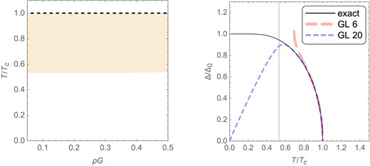
Left: Region in which the GL solution converges for BCS theory. The black dashed line denotes the second-order phase transition, and the orange shaded region indicates where the GL solution converges with Δ > 0. Right: BCS gap versus temperature, computed by solving the gap equation using the exact free energy (black), a 6th-order GL expansion (pink, dashed), and a 20th-order GL expansion (blue, dotted). The GL solution should converge to the right of the vertical gray line, i.e. T/T_c ≥ 0.53. These data are computed for ρG = 0.18.

Open in new tabDownload slide

Let us also comment on how the GL solutions in the right panel of Fig. 1 are calculated. Since solving the stationary equation ∂F/∂Δ = 0 for an Nth-order GL expansion involves finding the roots of an (N − 1)th-order polynomial in Δ, one should expect in general to find up to N − 1 potential solutions. Moreover, if the largest coefficient in such an Nth-order GL expansion is negative, then the free energy must eventually decrease toward −∞ as Δ → ∞, so one cannot determine the GL solutions simply by finding the global minimum. Instead, we essentially just search for the local minimum with the smallest free energy over 0 ≤ Δ ≤ Δ_conv. Although many more real roots of the stationary equation can appear with increasing N, in practice these occur far outside the radius of convergence, and hence they are easily neglected. The only additional complication is that the minimum in the 20th-order case gradually shifts and moves outside the convergence region as T/T_c drops below 0.53, and we continue to plot this minimum in the right panel of Fig. 1 (blue dotted curve left of the vertical line). We treat this as the solution because it remains close to the convergence region and is continuously connected to the solution at higher T. Note that this minimum remains well defined at all T because α₂₀ is positive; by contrast, the red dashed curve vanishes for T/T_c < 0.69 because the relevant local minimum at 6th order truly vanishes at these temperatures.

3. GL expansion in the NJL model

In this section, we show how the expression J₂(x, y) appears in the GL expansion for the dynamical quark mass in the NJL model and how it can be regularized in this setting. We then solve for the nth-order GL coefficients and convergence radius.

3.1. Microscopic theory and free energy

The two-flavor NJL Lagrangian is given by [7,12–14]:

Here ψ = (u, d)^⊤ is a two-flavor quark field, |$\hat{m} = \operatorname{diag}(m_{\rm u}, m_{\rm d})$| is the bare quark mass matrix in flavor space, G is a four-fermion coupling constant, and τ^a are the Pauli matrices acting in flavor space. This model retains the approximate chiral symmetry of QCD, which becomes exact in the chiral limit |$\hat{m} \rightarrow 0$|⁠. We will assume the chiral limit from now on.

In vacuum, chiral symmetry is spontaneously broken by the formation of a quark–antiquark pairing |$\sigma = \langle \bar{\psi }\psi \rangle$|⁠, called the chiral condensate. To study the behavior of the condensate σ as a function of temperature T and quark chemical potential μ, we expand Eq. (23) about the ansatz:

We note that at sufficiently large densities, or even small finite densities and in the presence of a magnetic field, this ansatz is known to be disfavored over various spatially inhomogeneous condensates within the mean-field approximation [15], the simplest being the so-called chiral density wave, given by |$\langle \bar{\psi }\psi \rangle + i \langle \bar{\psi } i \gamma ^5 \tau ^3 \psi \rangle = \sigma e^{iqz}$|⁠. In this paper, we restrict to the homogeneous case for simplicity.

In the mean-field approximation, one can show that the free energy is given by [13,14]:

where M = −2Gσ can be interpreted as the dynamical mass of quarks due to the chiral condensate; N_f = 2 and N_c = 3 are the numbers of flavors and colors, respectively; and |$E_{\boldsymbol k} = \sqrt{\boldsymbol k^2 + M^2}$|⁠. Making the transformations x = βk and y = βμ, we find

Here, the divergence of J₂ reflects the zero-point vacuum energy, and this divergence must be regularized in order to carry out numerical calculations. Several schemes are in common use [12]. For consistency with the last section, we will impose a simple momentum cutoff Λ, and take Λ → ∞ on any terms that remain finite in this limit. Such a cutoff clearly violates Lorentz invariance, which can lead to undesired consequences when the condensate under consideration is inhomogeneous [15]. In that context, covariant regularization methods, such as the Schwinger proper time method [16], are typically used instead. Since we consider only homogeneous condensates in this paper, the following analytical results based on a simple cutoff are physically meaningful. However, the numerical accuracy of the approximation Λ = ∞ is somewhat limited in this setting, as we will discuss in Sect. 3.3. It is also possible to solve for the GL coefficients using the proper time method, and in fact, that allows for analytical formulas for the GL coefficients even without taking the limit Λ → ∞; these results are given in Appendix  A. For the sake of accuracy, we use the proper time method in the numerical results presented in Fig. 2.

Fig. 2.

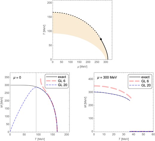
Top: Region in which the GL solution for the dynamical quark mass converges in the NJL model using Schwinger proper time regularization. The black curve shows the critical temperature, with solid (dashed) lines indicating the first-order (second-order) phase transitions. The orange shaded region indicates where the GL solution converges when M > 0. Bottom: Dynamical quark mass versus temperature at μ = 0 (left) and |$\mu = 300\, \text{MeV}$| (right), computed by solving the gap equation using the exact free energy (black), a 6th-order GL expansion (pink, dashed), and a 20th-order GL expansion (blue, dotted).

Open in new tabDownload slide

Imposing the momentum cutoff |$|\boldsymbol k| \lt \Lambda$| in Eq. (25), we find

3.2. nth-order coefficient formulas

As in the previous case, the GL expansion takes the form

The coefficient α₄ was previously computed in Ref. [17], but the expression for the generic coefficient α_2n has not been calculated explicitly, to the best of our knowledge. These coefficients are determined by the expansion coefficients of |$J_2^\text{cut}(x, y; \lambda )$| in powers of x,

via

which we will now derive. Finally, once the c_2n coefficients are known, the α_2n coefficients follow immediately from Eq. (27),

The two differences from the BCS case are that we now have J₂ rather than J₀, and we now have y ≠ 0. The appearance of J₂ adds a factor of t² to the integrand, which strengthens the UV divergence, and as a result, we will need to keep λ finite on the c₄ coefficient in addition to c₂. Having y ≠ 0 complicates the algebra, but does not significantly affect the overall approach.

Following the same procedure as in the BCS case, we start by taking a single derivative with respect to x², giving

where |$\bar{\omega }_k = (2k + 1)\pi$|⁠, as before. After applying the identity

we obtain

At this point, in close analogy to the comment after Eq. (12), we may see a hint of the final result for the radius of convergence. If one expands the integrand in powers of x², the resulting series has radius of convergence |$x_\text{conv}^2 = |t^2 + (\bar{\omega }_k + iy)^2|$|⁠. Taking t → 0 then gives |$x_\text{conv}^2 = |\bar{\omega }_k + iy|^2$|⁠, the minimum of which is |$x_\text{conv}^2 = \pi ^2 + y^2$|⁠; recalling that x = βM and y = βμ, this corresponds to |$M_\text{conv} = \sqrt{\mu ^2 + (\pi T)^2}$|⁠. However, this heuristic argument is fairly crude, partly because the quantity |$|t^2 + (\bar{\omega }_k + iy)^2|$| need not be minimized in the limit t → 0. We therefore proceed to the rigorous proof.

Taking n − 1 more derivatives of Eq. (34) with respect to x², introducing a variable |$s = t/(\bar{\omega }_k + iy)$|⁠, and letting λ → ∞, we find

The integral is easily performed by using Eq. (13), giving

Notice that the sum in Eq. (35) converges when n ≥ 3. Identifying the sum with the standard series representation of the nth-order polygamma function |$\psi ^{(n)}(z) = (-1)^{n+1} n! \sum _{k=0}^{\infty } 1/(z+k)^{n+1}$|⁠, we finally find

For c₂ and c₄, it is more convenient to avoid writing J₂ as a Matsubara sum, starting instead from the expression

For c₂, it is straightforward to calculate

where |$\operatorname{Li}_n(x) = \sum _{k=1}^{\infty } x^k/k^n$| is the nth polylogarithm. The first two terms under the sum in Eq. (39) vanish as λ → ∞, and for the last term we can apply the identity [18],

where B_n(x) is the nth Bernoulli polynomial. The result is

The c₄ coefficient is more subtle because a naive separation of Eq. (38) into vacuum and medium contributions leads to IR divergences. An efficient way to compute this coefficient is to note that after commuting the derivatives |$\partial _{x^2}^2$| with t² in the integrand, we can transform them as |$\partial _{x^2} \rightarrow (2t)^{-1} \partial _t$|⁠. This allows us to take the limit x → 0 and then take derivatives with respect to t. Performing only the rightmost derivative, we find

Integrating by parts, taking λ → ∞ on the boundary terms, and by applying the formula [19],

where ψ(z) is the digamma function defined by ψ(z) = dln Γ(z)/dz with Γ(z) the gamma function, we obtain

for large λ, and accordingly,

Finally, applying Eq. (31), we have

3.3. Radius of convergence

We will show that the expansion of |$J_2^\text{cut}(x, y; \lambda )$| has radius of convergence |$x_\text{conv} = \sqrt{\pi ^2 + y^2}$|⁠. Then, from Eq. (27), it will follow that the GL expansion has convergence radius |$M_\text{conv} = (x_\text{conv}|_{y = \beta \mu }) T = \sqrt{\mu ^2 + (\pi T)^2}$|⁠.

First, since the convergence of any series only depends on its infinite tail, and not on any finite initial segment, we can focus on the coefficients c_{2n ≥ 6} given by Eq. (37). It is straightforward to show that the radius of convergence is at least  |$\sqrt{\pi ^2 + y^2}$|⁠. Using the inequality |$|\operatorname{Re} (z)| \le |z|$| for complex z, we have

for 2n ≥ 6.

Using the identity |$\psi ^{(n)}(x) = (-1)^{n+1} n! \, \zeta (n + 1, x)$|⁠, where |$\zeta (s,a)=\sum _{k=0}^{\infty }1/(k+a)^{s}$| is the Hurwitz zeta function, one can show that

for |$\operatorname{Re}(x) \gt 0$|⁠, in the sense that the ratio of the quantities on the left and right sides of the arrow approaches unity as n → ∞. It follows that

Thus, the series for |$J_2^\text{cut}(x, y; \lambda )$| in Eq. (29) is bounded in magnitude by a series with radius of convergence |$x_\text{conv} = \sqrt{\pi ^2 + y^2}$|⁠, so the original series has a convergence radius of at least this value. In fact, one can show the exact convergence radius is indeed |$\sqrt{\pi ^2 + y^2}$|⁠, but the proof is more involved. In particular, if we do not take the upper bound of the coefficients using |$|\operatorname{Re} (z)| \le |z|$|⁠, then the ratio test does not work, because the quantity |$[\operatorname{Re} \psi ^{(2n - 4)}(\frac{1}{2} + i\frac{y}{2\pi })] / [\operatorname{Re} \psi ^{(2n - 2)}(\frac{1}{2} + i\frac{y}{2\pi })]$| oscillates erratically. One can instead use the Cauchy–Hadamard theorem; we sketch this proof in Appendix B.1.

Although the results of this section were computed using a simple momentum cutoff Λ, the radius of convergence is unaffected when using Schwinger proper time regularization. Whereas the former cutoff scheme involves taking the limit Λ → ∞ to obtain parts of c_2n and α_2n analytically, the latter scheme allows deriving their analytic expressions even without taking such a limit for a cutoff parameter Λ. As shown in Appendix  A, the α_{2n ≥ 6} coefficients are almost the same as in Eq. (48), except with small corrections proportional to inverse powers of Λ. The key fact is that these correction terms decay faster than the α_2n coefficients calculated in this section, so they do not increase the convergence radius. We prove these statements in Appendix  A.

Let us also mention that the assumption of Λ = ∞ made when deriving Eqs. (46)–(48) is only a rough approximation in the NJL setting. The values for the two parameters Λ and G are determined by a choice of values for M₀ and f_π, where M₀ is the dynamical quark mass and f_π is the pion decay constant at T = μ = 0. Choosing |$M_0 = 300\, \text{MeV}$| and |$f_\pi = 88\, \text{MeV}$| in the chiral limit [15,20], we find |$\Lambda = 614\, \text{MeV}$| and GΛ² = 2.15 [12]. With these values, one can numerically find |$T_{\rm c} = 182\, \text{MeV}$| at μ = 0, and |$\mu _{\rm c} = 311\, \text{MeV}$|⁠, where μ_c is the chemical potential at which M vanishes in a first-order transition with T = 0 fixed. Thus, Λ is not especially large on the scale of other characteristic quantities of the system, so taking Λ → ∞ is not fully justified. For instance, finding T_c by setting α₂ = 0 in Eq. (46) gives |$T_{\rm c} = 165\, \text{MeV}$|⁠. Although the series with coefficients given by Eqs. (46)–(48) converges with radius |$\sqrt{\mu ^2 + (\pi T)^2}$|⁠, the value does not converge exactly to Ω, even within this radius.

These issues are avoided when using Schwinger proper time regularization, described in Appendix  A, because there the finite size of Λ is captured in the analytical formulas for the coefficients. Therefore, the numerical results for this section, presented in Fig. 2, are computed using the Schwinger method. In this regularization scheme, again choosing |$M_0 = 300\, \text{MeV}$| and |$f_\pi = 88\, \text{MeV}$|⁠, we find |$\Lambda = 634\, \text{MeV}$| and GΛ² = 6.02. We calculated T_c over the range |$0 \le \mu \le 312\, \text{MeV}$|⁠, and we determined the region in the μ-T plane below T_c where M < M_conv, i.e. where the GL solution converges (top panel, orange shaded region). The bottom panels of Fig. 2 show M vs. T computed from the gap equation and also from the GL expansion at orders 6 and 20. For μ = 0 (bottom left panel), the GL solution converges only when |$T \gt 92\, \text{MeV}$| (right of the vertical line); both the 6th- and 20th-order solutions are very accurate near T_c, but the 6th-order solution becomes noticeably inaccurate at |$T \lesssim 130\, \text{MeV}$|⁠. On the other hand, when |$\mu = 300\, \text{MeV}$| (bottom right panel), the phase transition is first order, and the 20th-order solution is a noticeable improvement over the 6th-order solution across the entire range 0 < T < T_c. Moreover, the GL solution converges over this entire range, and hence the 20th-order solutions are very reliable all the way down to T = 0. This can be understood by considering the radius of convergence formula at T = 0, which reduces to M_conv = μ, and noticing that |$M \le 300\, \text{MeV}$| for |$\mu \gt 300\, \text{MeV}$|⁠.

We also note that the method used for determining the solutions of the 6th- and 20th-order GL expansions, plotted in the lower panels of Fig. 2, is exactly the same as in the BCS case, as discussed in the last paragraph of Sect. 2.3.

As mentioned above and shown in Appendix  A, the radius of convergence when using the proper time method is also |$\sqrt{\mu ^2 + (\pi T)^2}$|⁠. One could also ask about the radius of convergence in the cutoff method if not using the approximation Λ = ∞, i.e. if instead one were to calculate the GL coefficients from Eq. (27) numerically at finite Λ. It is possible to show that in this case the radius of convergence is still given by at least |$\sqrt{\mu ^2 + (\pi T)^2}$| when M > 0; we sketch a proof in Appendix B.2.

4. Discussions and outlook

In this paper, we studied the convergence of the GL expansion for two prominent examples—the BCS theory for superconductivity and the NJL model for chiral symmetry breaking at finite temperature T and chemical potential μ. We have shown that the convergence radii are given by Δ_conv = πT and |$M_{\rm conv} = \sqrt{\mu ^2 + (\pi T)^2}$|⁠, respectively. The difference between these two expressions can be understood physically as follows. In the BCS theory, Cooper pairing occurs close to the Fermi surface, so μ dependence enters only through the density of states, which is universal for all the GL coefficients. In the NJL model, on the other hand, the chiral condensate is a pairing between quarks and antiquarks inside the Dirac sea, so the GL coefficients depend rather nontrivially on μ, as shown in Eqs. (46)–(48). We also note that this difference leads to the known fact that the BCS instability appears for an infinitesimally small attractive interaction between fermions, whereas generation of the chiral condensate requires a sufficiently strong attractive interaction between quarks and antiquarks [7].

In this paper, we focused on the two-flavor NJL model, where only even powers of M appear in the GL expansion. In the three-flavor case, on the other hand, odd powers in M can also appear in the expansion [21] due to the instanton-induced interaction (or Kobayashi–Maskawa–’t Hooft interaction) [22–24]. It would be interesting to see how the radius of convergence may be affected by such terms. One can also ask about the radius of convergence of the GL theory for the chiral phase transition in QCD per se. For the mean-field approximation to be well justified, one can take the large-N_c limit [25,26]. Because the radius of convergence for the dynamical quark mass in the NJL model above does not depend on the details of the model, such as the four-fermion coupling constant G and cutoff Λ,³ one may conjecture that large-N_c QCD has the same radius of convergence, |$M_{\rm conv} = \sqrt{\mu ^2 + (\pi T)^2}$|⁠.⁴

It would be interesting to extend our approach to the diquark condensate for color superconductivity [28], the interplay between chiral and diquark condensates [29], the inhomogeneous condensates like Fulde–Ferrell–Larkin–Ovchinnikov (FFLO) pairing [30,31] or inhomogeneous chiral condensates [15], and other orders in condensed matter systems. We defer these questions to future work.

Acknowledgement

We thank T. Brauner for useful correspondence and comments on the manuscript. Furthermore, we acknowledge support from JSPS through the JSPS Summer Program 2023, where this collaboration was initiated.

Funding

Open Access funding: SCOAP³. N.Y. is supported in part by the Keio Institute of Pure and Applied Sciences (KiPAS) project at Keio University and Japan Society for the Promotion of Science (JSPS) KAKENHI grant numbers JP19K03852 and JP22H01216.

Appendix A. GL coefficients in the NJL model from the proper time method

The general idea of the proper time regularization amounts to making the following replacement by introducing a UV cutoff Λ:

For our purpose, we need the |$n=-\frac{1}{2}$| case,

for only the first term of Eq. (25), where we used |$\Gamma (-\frac{1}{2})=-2\sqrt{\pi }$|⁠. The replacement in Eq. (A2) arises more naturally when deriving the free energy Ω in the proper time framework, where the divergences appear as integrals of the form |$\int _0^\infty \frac{ds}{s^{3/2}} e^{-sE_{\boldsymbol k}^2}$| (see, e.g. Appendix A of Ref. [32]).

We can now express the free energy as a well-defined quantity,

where

Let us introduce the function

where |$\operatorname{erfc}(x) = \frac{2}{\sqrt{\pi }}\int _x^{\infty }dt\, e^{-t^2}$| is the complementary error function, and we have suppressed the dependence on L and y to reduce clutter. One can show that |$t^2 \mathrm{ F}(\sqrt{x^2 + t^2})$| is precisely the integrand of |$J_2^\text{Schw}(x, y; L)$|⁠, and this allows us to write |$J_2^\text{Schw} = \frac{1}{2} \int _{- \infty }^{+ \infty } dt \, t^2 \mathrm{ F}(\sqrt{x^2 + t^2})$|⁠. Note also that F(z) is an even function of z that vanishes rapidly at ±∞, which are important properties in what follows.

We then need to compute |$\partial _{x^2}^n \mathrm{ F}(\sqrt{x^2 + t^2}) \big |_{x = 0} = 2^{-n}(t^{-1} \partial _t)^n \mathrm{ F}(t)$|⁠. The n = 1 case combined with an integration by parts immediately yields

For the higher coefficients, we can put (t⁻¹∂_t)ⁿ into the form |$t^{-1} \partial _t^{2n + 1}$| using repeated integration by parts. One can show that [19,33]:

The above integrals |$\int _{- \infty }^{+ \infty } dt \mathrm{ F}(t)$| and |$\int _{-\infty }^{+ \infty } dt\, t^{-1} \partial _t^n \mathrm{ F}(t)$| can be analytically performed for all n [19]:

We therefore have

and

It now follows from Eq. (A3) that the GL coefficients are given by

Explicitly,

Note that the only differences between these coefficients and those given in Eqs. (46)–(48) are in the terms involving Λ, as expected. We also note that these coefficients can be regarded as a special case of those derived in Refs. [19,33] for the case of an inhomogeneous chiral condensate in a magnetic field, after setting B = 0 and considering only terms in the GL expansion that do not contain any gradients.

Let us now focus on the coefficients c_{2n ≥ 6} and consider the convergence of the corresponding series. Since each coefficient is a sum of two parts, |$c_{2n \ge 6} = c_{2n}^\text{vac} + c_{2n}^\text{med}$|⁠, the series for |$J_2^\text{Schw}(x, y; L)$| can be separated into two subseries,

This rearrangement of terms is justified because rearrangements can only affect a conditionally convergent series (or more accurately, a series for which some rearrangement converges conditionally), and power series can only converge conditionally at their exact radius of convergence. Thus, rearranging a power series cannot change its convergence radius. It is easy to check that the first subseries, whose coefficients are |$c_{2n}^\text{vac}$|⁠, has infinite radius of convergence, e.g. by applying the ratio test. Therefore, the convergence radius of the original series is determined by that of the second subseries, whose coefficients are |$c_{2n}^\text{med}$|⁠. But |$c_{2n\ge 6}^\text{med}$| are precisely the coefficients c_{2n ≥ 6} that were calculated in Sect. 3.2 using the momentum cutoff, so the radius of convergence here is the same as in the previous case.

Appendix B. Convergence radius for the GL expansion in the NJL model

When computing the GL coefficients for the NJL model in Sect. 3.2, we approximated Λ as being very large compared to other characteristic quantities of the system, resulting in the coefficients given by Eqs. (46)–(48). Let us denote the radius of convergence associated with these coefficients by |$M_\text{conv}^{\text{cut,}\Lambda \rightarrow \infty }$|⁠. One can also consider the radius of convergence of the GL expansion obtained using cutoff regularization, but without taking the limit Λ → ∞ (although we have not found simple analytical formulas for the coefficients in this case). Let us denote the latter radius of convergence by |$M_\text{conv}^{\text{cut}}$|⁠. Finally, let us denote by |$M_\text{conv}^\text{Schw}$| the radius of convergence of the GL expansion when using the Schwinger proper time regularization scheme.

Using the above notation, we can summarize the previous results as follows:

(i) was shown at the end of Appendix  A, and (ii) was shown at the end of Sect. 3.3. In the first part of this appendix, we show that equality holds in (ii), i.e. |$M_\text{conv}^{\text{cut,}\Lambda \rightarrow \infty } = \sqrt{\mu ^2 + (\pi T)^2}$|⁠. In the second part of this appendix, we consider the case of cutoff regularization without assuming Λ → ∞, and we show that |$M_\text{conv}^{\text{cut}} \ge \sqrt{\mu ^2 + (\pi T)^2}$| over the region in the μ-T plane where M > 0, after fixing Λ and G such that |$M_0 = 300\, \text{MeV}$| and |$f_\pi = 88\, \text{MeV}$|⁠.

B.1. Cutoff regularization with Λ → ∞

According to the Cauchy–Hadamard theorem, the radius of convergence of the series c₂x² + c₄x⁴ + ⋅⋅⋅ is given by

Applying this theorem to c_2n given by Eq. (37), and using the formula |$\psi ^{(n)}(x) = (-1)^{n + 1} n! \, \zeta (n + 1, x)$| and the fact that |$\sqrt[n]{|a|} \rightarrow 1$| as n → ∞ for any a ≠ 0, we find

It is easy to show that the first factor in the limit approaches 1. For the second factor, the terms except for j = 0 in the sum over j become negligible as n → ∞, so we have

where |$z = 1/\left({\tfrac{1}{2} + i\tfrac{y}{2 \pi }} \right)$| and |$\hat{z} = z / |z| = e^{2\pi i\phi }$| is a complex phase of unit magnitude. The result will follow if we can show that the remaining lim sup evaluates to unity. First, we have |$\sqrt[2n]{|\operatorname{Re}(\hat{z}^{2n - 3})|} \le \sqrt[2n]{|(\hat{z}^{2n - 3})|} = 1$|⁠, so we must only show that |$\sqrt[2n]{|\operatorname{Re}(\hat{z}^{2n - 3})|}$| contains a subsequence converging to 1. If ϕ is rational, then |$\hat{z}^{2n - 3}$| will cycle through finitely many values infinitely many times. Letting |$a = |\operatorname{Re}(\hat{z})|$|⁠, there is a subsequence |$\sqrt[2n]{a}$|⁠, which converges to 1. If ϕ is irrational, then the set of points |$\lbrace e^{2\pi i\phi n} \, | \, n \in \mathbb {N} \rbrace$| is dense in the unit circle, and hence so is the set |$\lbrace e^{2\pi i\phi (2n - 3)} \, | \, n \in \mathbb {N} \rbrace$|⁠. Thus we can choose a subsequence {a_n} of e^{2πiϕ(2n − 3)} whose elements all have real part at least |$\frac{1}{2}$|⁠, and then |$\sqrt[2n]{|\operatorname{Re}(a_n)|} \rightarrow 1$|⁠.

B.2. Cutoff regularization with finite Λ

Starting from Eq. (34) and repeating the calculation without taking λ → ∞, we find

where we have defined A_k ≔ (2k + 1)π + iy. Because λ/A_k is complex, the integral in Eq. (B5) must now be interpreted as a contour integral. Let C_k be some contour that starts at the origin, ends at λ/A_k, and avoids the poles at |$s = \pm i$|⁠; we will consider two different choices of C_k. Let |C_k| denote the length of the contour C_k.

Applying the Cauchy–Hadamard theorem (B2), we have

Recall that Eq. (B6) holds for any valid choice of contours C_k. Let us first consider contours that follow the straight line from the origin to λ/A_k. If y ≤ π, then y ≤ (2k + 1)π for all k, and it is easy to show that |1 + s²| ≥ 1 for all s ∈ C_k. We therefore have

which shows that |$x_\text{conv} \ge \sqrt{\pi ^2 + y^2}$| if y ≤ π.

More generally, for any |$y \in \mathbb {R}$|⁠, one can derive the weaker lower bound

from which we find

Thus, we always have |$x_\text{conv} \ge \sqrt{2\pi y}$|⁠, or equivalently, |$M_\text{conv} \ge \sqrt{2\pi \mu T}$|⁠. It is easy to check that the previous lower bound |$x_\text{conv} \ge \sqrt{\pi ^2 + y^2}$|⁠, which holds (at least) if y ≤ π, is always an improvement over |$\sqrt{2\pi y}$| (except precisely at y = π, where the two bounds are equal).

Finally, by considering a different choice of the contour C₀, one can show that the improved lower bound |$x_\text{conv} \ge \sqrt{\pi ^2 + y^2}$| holds over a larger region of parameter space. Let C₀ now be the contour that runs first along the positive real axis from 0 to |λ/A₀|, and then along a circular arc of constant radius from |λ/A₀| to λ/A₀ (we let C_k for k > 0 be the same as before). It is then easy to show that if |$|\lambda / A_0| \ge \sqrt{2}$|⁠, then again |1 + s²| ≥ 1 for all s ∈ C₀. We also have |C_k| ≤ (1 + π/2)|λ/A_k| for all k, from which we find

We have shown that |$x_\text{conv} \ge \sqrt{2\pi y}$| for all |$y \in \mathbb {R}$|⁠, and that the improved lower bound |$x_\text{conv} \ge \sqrt{\pi ^2 + y^2}$| holds if y ≤ π or |$|\lambda / A_0| \ge \sqrt{2}$| (in fact, these conditions are sufficient, but not necessary). The condition |$|\lambda / A_0| \ge \sqrt{2}$| is equivalent to |$y \le \sqrt{\frac{1}{2} \lambda ^2 - \pi ^2}$|⁠, and it follows that

Fig. B1 shows the region in the μ-T plane where the two conditions in Eq. (B11) hold, along with T_c computed using cutoff regularization.

Fig. B1.

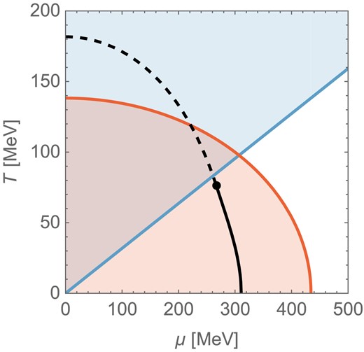
Convergence behavior of the GL expansion using cutoff regularization without assuming Λ = ∞. In the shaded regions corresponding to the conditions given in Eq. (B11), we have |$M_\text{conv}^\text{cut} \ge \sqrt{\mu ^2 + (\pi T)^2}$|⁠, and in the unshaded region we have the weaker lower bound |$M_\text{conv}^\text{cut} \ge \sqrt{2\pi \mu T}$|⁠. The blue shaded region corresponds to |$T \geq \mu / \pi$|⁠, and the red shaded region corresponds to |$T \leq \frac1\pi \sqrt{\frac12 \Lambda^2 - \mu^2}$|⁠. The black curve shows T_c, computed by solving the gap equation numerically with cutoff regularization, with solid (dashed) lines indicating the first-order (second-order) transitions. We use |$\Lambda = 614\, \text{MeV}$| and GΛ² = 2.15 as described in Sect. 3.3.

Open in new tabDownload slide

Footnotes

References