


Abstract
In recent years, advances in computing hardware and computational methods have prompted a wealth of activities for solving inverse problems in physics. These problems are often described by systems of partial differential equations (PDEs). The advent of machine learning has reinvigorated the interest in solving inverse problems using neural networks (NNs). In these efforts, the solution of the PDEs is expressed as NNs trained through the minimization of a loss function involving the PDE. Here, we show how to accelerate this approach by five orders of magnitude by deploying, instead of NNs, conventional PDE approximations. The framework of optimizing a discrete loss (ODIL) minimizes a cost function for discrete approximations of the PDEs using gradient-based and Newton’s methods. The framework relies on grid-based discretizations of PDEs and inherits their accuracy, convergence, and conservation properties. The implementation of the method is facilitated by adopting machine-learning tools for automatic differentiation. We also propose a multigrid technique to accelerate the convergence of gradient-based optimizers. We present applications to PDE-constrained optimization, optical flow, system identification, and data assimilation. We compare ODIL with the popular method of physics-informed neural networks and show that it outperforms it by several orders of magnitude in computational speed while having better accuracy and convergence rates. We evaluate ODIL on inverse problems involving linear and nonlinear PDEs including the Navier–Stokes equations for flow reconstruction problems. ODIL bridges numerical methods and machine learning and presents a powerful tool for solving challenging, inverse problems across scientific domains.
Inverse problems are fundamental in science and engineering, often revealing solutions unattainable through direct methods. Inspired by efforts to solve such problems using physics neural networks (PINNs), we present the framework of optimizing a discrete loss (ODIL). ODIL deploys conventional discretizations on a grid instead of neural networks. ODIL is a drop-in replacement for PINNs in many scientific and engineering problems, while being several orders of magnitude more efficient in terms of computational cost and achieving higher accuracy.
Introduction
The numerical solution of physical models expressed as partial differential equations (PDEs) is indispensable across all areas of science, engineering, and medicine. Commonly, solutions are presented for the so-called forward problems where the PDEs are discretized on grids or particles (1–3), and the discrete problems are solved to determine quantities of interest given initial and/or boundary conditions. In recent years, the advent of data science has prompted intense interest in solving PDEs in the context of “inverse problems” where the parameters and even the structure of PDE models are inferred from data (4–7). Solving inverse problems in science and engineering entails formidable challenges as the PDEs need to be solved while observing physical and geometrical constraints as well as noisy data (8). Such problems are encountered in several fields of science and engineering, and they have been handled by methods such as PDE-constrained optimization (9), data assimilation (10), optical flow in computer vision (11), and system identification (12). As there is an ever increasing number of problems that involve noisy or missing data, there is a strong need to develop efficient methods for solving such problems and machine learning has emerged as a potent modality (7, 13, 14), albeit with certain limitations (8).
Physics-informed learning using neural networks (NNs) for partial and ordinary differential equations were introduced three decades ago, by Dissanayake and Phan-Thien (15), van Milligen et al. (16), and Lagaris et al. (17). In these works, the unknown fields were represented by NNs with weights obtained by minimizing a loss function composed by the residuals of the governing equations. Related efforts used NNs for modeling nonlinear dynamical systems (18, 19), back-tracking of an N-body system (20), and deep NNs for reconstructing the flow field in the near-wall region of a turbulent flow using wall only information (21). At the time of their introduction, these methods were not favored for solving forward or inverse problems, in particular due to their computational cost and the speed of available computing architectures. Twenty years later, the method was revived by Raissi et al. (22) who used modern machine-learning methods and software (such as deep neural networks, automatic differentiation, and TensorFlow) to carry out its operations. The method has been popularized by the term physics-informed neural network (PINN).
PINNs have created a lot of enthusiasm in the scientific community as they offered an alternative to solving complex physical problems using convenient representations at a significantly reduced cost of implementation. However, it is broadly accepted that PINNs cannot match conventional numerical methods for solving well-posed forward problems involving PDEs but they are positioned as a convenient tool for solving ill-posed and inverse problems and data-driven modeling (7). The proper assessment of this claim hindered by the fact that to date there is no baseline for assessing the capabilities of PINNs with respect to conventional methods for solving forward and inverse problems. Raissi et al. (22) admit that conventional numerical solvers are more efficient for forward problems, a direct comparison with such solvers reveals important drawbacks of the neural network approach (23).
The overall computational cost of PINNs originates from the cost of evaluating the solution in each collocation point. Represented by a fully connected network, the solution in each point depends on all weights of the neural network, therefore the cost of evaluating it in one point is proportional to the number of weights. In contrast to neural networks, conventional grid-based methods represent the solution with local approximations resulting in a constant cost per point. Consequently, the gradient of the residual with respect to the weights in one point is a dense vector and the Hessian of the loss function a dense matrix. This makes higher order optimization methods such as Newton’s method unsuitable for training NNs. Furthermore, the convenience of representation and ease of formalism by PINNs comes with limitations. While PINN evaluates the differential operator exactly on a set of collocation points, it makes no allowance for physically and numerically motivated adjustments that speed up convergence and ensure discrete conservation such as deferred correction, upwind schemes, and discrete conservation laws as represented, for example, in the finite volume method. Furthermore, decades of development and analysis that went into conventional solvers enables understanding, prediction, and control of their convergence and stability properties. Such information is not available with neural networks and recent works aim to remedy this situation (24, 25). Application of PINN to equations with high-order derivatives is also limited (26, 27) as the computational cost of nested automatic differentiation is exponential in the order of differentiation (28, 29), while in the case of finite differences, the cost is linear.
More recently, the architectures deployed in PINNs have undergone significant enhancements, including the introduction of positional encodings, exact enforcement of boundary conditions, incorporation of adaptive activation functions, and improving the treatment of constraints and invariances (30–34). While these techniques significantly improve the performance in certain cases, they do not guarantee a universal improvement in accuracy or training speed. When it comes to studies involving PINNs, it is generally not advisable to start with these techniques, considering the numerous hyperparameters that already require tuning. For instance, there are cases where enforcing exact boundary conditions can lead to worse performance. In such scenarios, a more effective approach may involve blending the boundary conditions into the approximation, even if it diverges from the reference solution. The same principle applies to positional encodings, which entail adding sine waves to the input. While this approach clearly boosts performance in scenarios like the wave equation with periodic boundary conditions, where the solution is a linear combination of sine waves, it may not yield the same benefits for more general conditions. Nevertheless, in our experimentation with PINNs, we applied several well-known algorithmic modifications. Our observations did not indicate any noteworthy enhancements, consistent with similar experiences by other groups (35–37). Moreover, the effects of these modifications were similar to the variations observed when changing the random seed (see SI Appendix). Our observations align with a recent paper authored by one of the co-creators of PINNs, wherein the attempt to solve the
Here, we present a framework that is based on conventional numerical methods that overcomes many of the challenges encountered by PINNs. We show that this valuable approach can be accelerated by five orders of magnitude by deploying conventional numerical algorithms that are facilitated by machine-learning tools. We cast the framework as optimizing a discrete loss (ODIL) by combining discrete formulations of PDEs with modern machine-learning tools to extend their scope to ill-posed and inverse problems.
The framework of ODIL minimizes a cost function for the discrete forms of PDEs using gradient-based and Newton’s methods. We demonstrate that ODIL is effective in solving inverse problems for equations with missing parameters and with limited data. This framework has two key aspects. First, the discretization itself that defines the accuracy, stability, and consistency of the method. Second, the optimization algorithm to solve the discrete problem. Our method uses efficient computational tools that are readily available for both of these aspects. The discretization properties are inherited from the conventional numerical methods building upon the advances in this field over multiple decades. Since the sparsity of the problem is preserved, the optimization algorithm can use a Hessian and achieve a quadratic converge rate, which remains out of reach for gradient-based training of neural networks. We remark that solving the discrete equations as a minimization problem is not a new idea. It has been developed in various forms in different domains, including the discretize-then-differentiate approach in the context of PDE-constrained optimization (9), as the penalty method (39), and is related to the 4D-VAR problem in variational data assimilation (10, 40), in addition to regularization techniques (41). Differentiable solvers (42–45) serve as a tool for computing the gradients of the solution with respect to parameters of the problem. They can be combined with a gradient-based optimization method to fit the solution to known data and infer the parameters. However, they assume that the forward problem is well-posed, which is not always the case as demonstrated by the “notorious test problem” in optimal control (46, 47) discussed in Fig. S4.
Another related approach is the neural bootstrapping method (NBM) (27, 48). NBM represents the solution with a neural network as in PINN but evaluates conventional discretization schemes on a set of random collocation points using a local stencil around each point. The authors have applied this approach to elliptic problems with discontinuities. Although NBM does not reduce the cost of evaluating the solution in each point introduced by a fully connected NN, it can be less computationally expensive than PINN if the equations contain high-order derivatives. The cost of nested automatic differentiation in PINN grows exponentially with the order of the derivative, but NBM uses finite differences for which the cost is linear. While the authors do not provide a direct comparison with conventional solvers in terms of the accuracy and computational cost, they use small neural networks (e.g. 1,000 parameters) and evaluate the loss on a grid with significantly more cells (e.g.
In the following, we present a potent computational framework for solving forward and inverse problems with missing and noisy data and facilitate its deployment by adopting machine-learning tools. Adopting modern machine-learning tools, such as automatic differentiation, renders the implementation of ODIL as convenient as applying gradient-based methods in PINNs, providing a baseline for the comparison of these methods. We present a number of solutions to prototypical and benchmark problems to evaluate the performance of ODIL. Our results indicate that ODIL outperforms PINNs by up to five orders of magnitude in computational speed and with better accuracy while covering the same class of inverse and ill-posed problems. Finally, we note that ODIL is an example of bridging numerical methods and machine learning. The successful fusion of these two domains with complementary potentials can create further developments of computational methods for challenging scientific and engineering problems described by PDEs.
Methods
Formulation of ODIL
Here, we formulate the ODIL framework to solve forward and inverse problems for PDEs. Using a given discretization of the PDEs, we construct a loss function from the residuals of the discretization, data terms, and regularization terms. The applications in this article involve discretizations on a uniform Cartesian grid, but this general formulation is applicable to other cases, e.g. an unstructured triangular grid. Let C denote the cell indices of a grid in a d-dimensional space
where
with the loss function
where
We consider two approaches to solving this minimization problem. The first approach is to use a standard gradient-based method, such as Adam (51) or L-BFGS-B (52), with the gradients of
The second approach is the Gauss–Newton method, which iteratively solves the problem by updating the solution based on linearization of the residual operators about the current solution. Let
where
which is now a quadratic function of
On the other hand, a minimum of
which is a system of linear equations. To derive the system, we combine all unknowns in one column vector
all residuals in one column vector
and the corresponding derivatives in one matrix
In this notation, the linearized operators (4) take the form
where
Finally, the optimality conditions (7) are now equivalent to
Solving this linear system for
Calculating sparse Jacobians
Discrete equations (1) that result from approximations of PDEs are often local, i.e. the residual in each cell depends on values of unknown fields in a limited number of neighboring cells. In such cases, the Jacobians with respect to the unknown fields in Eq. (10) are sparse. To calculate them, we intend to use automatic differentiation of scalar functions. Coloring techniques (57, 58) can be used to estimate a sparse Jacobian using multiple evaluations of a Jacobian-vector product. However, we use a more explicit approach that directly tracks the dependencies on the neighboring cells. For simplicity, assume that
where
and calculate the desired Jacobian as
where the derivatives of
Multigrid decomposition
Here, we propose a multigrid technique to accelerate the convergence of optimization methods for problems that involve discrete fields on a grid. Multigrid methods are generally accepted as the fastest numerical methods for solving elliptic differential equations (59). A standard multigrid method consists of the following parts: a hierarchy of grids including the original grid and coarser grids, discretizations of the problem on each grid, interpolation operators to finer levels, and restriction operators to coarser levels. The method iteratively updates the solution on each level, interpolates the update to finer levels, and restricts the residuals to coarser levels.
As discussed above, the optimization problem in ODIL can be solved with Newton’s method which involves a linear system at each step, so the multigrid method can be applied directly to that linear system. However, then we need to construct the linear system explicitly and rely on a general multigrid solver which may have limited efficiency especially on GPUs (60). Furthermore, if the equation involves unknown parameters, such as parameters of a neural network, as demonstrated on the problem of inferring conductivity from temperature, in Results, the corresponding Jacobian matrix is dense, which makes Newton’s method impractical.
Instead of Newton’s method, we can solve the problem with a general optimization algorithm, such as Adam or L-BFGS. However, as we demonstrate on the lid-driven cavity flow in Results, they require orders of magnitude more iterations than Newton’s method. To accelerate the convergence, we propose the following technique. Consider a uniform grid with
where each
Note that this representation is over-parameterized and therefore not unique. The total number of scalar parameters increases from
Results
Wave equation: accuracy and cost of PINN
We apply ODIL and PINN to solve an initial-value problem for the wave equation in two dimensions and compare both methods in terms of accuracy and computational cost. The problem consists of the wave equation
with the initial conditions and boundary conditions
in a rectangular domain
Both methods reduce the problem to minimization of a loss function. ODIL represents the solution on a uniform Cartesian grid of size
for
for
using second-order extrapolation. ODIL solves the minimization problem for the loss function [3] computed from this residual operator. We choose
Figure 1 presents examples of the solutions obtained using both methods and also shows how the error and execution time of both methods depend on the number of parameters. The results of PINN include 25 runs with random initial weights and positions of the collocation points. In the case of ODIL, solutions from two optimization methods, L-BFGS-B and Newton, coincide. For each run of PINN or ODIL with L-BFGS-B, we determine the best error achieved during 80,000 epochs and estimate the required number of epochs as the number of epochs to achieve 150% of the best error. Then, we estimate the execution time per epoch as the mean over the last 100 epochs for L-BFGS-B and one epoch for Newton’s method, excluding the time spent on startup, building the computational graph, and output. The measurements are performed on one CPU core of Intel Xeon E5-2690 v3 and exclude the startup time spent on building the computational graph required on the first epoch. We report the execution time as the product of the required number of epochs and the execution time per epoch. Both methods demonstrate similar accuracy. The error of ODIL scales as
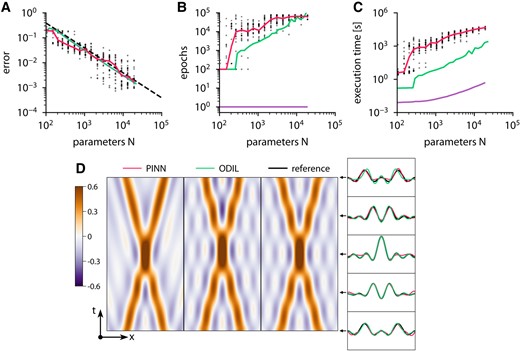
Wave equation solved using PINN and ODIL. A–C) Root-mean-square error relative to the exact reference solution (A), required number of epochs (B), and execution time on one CPU core (C) of various methods: PINN with L-BFGS-B  , ODIL with L-BFGS-B
  , ODIL with Newton
  , and line with slope
  . For PINN, the dots show samples with random initial weights and collocation points, and solids lines show the median value. The number of parameters is the number of weights for PINN and the number of grid cells for ODIL. D) Solution obtained using PINN with L-BFGS-B with two hidden layers of 25 neurons, ODIL with Newton on a grid of , and exact reference solution
  .
.
Poisson equation in two dimensions
We apply ODIL and PINN to solve the boundary-value problem for the Poisson equation
with zero Dirichlet boundary conditions in a unit domain
with
Figure 2 shows results of both methods compared to the reference solution along with the convergence history. The error is measured relative to the exact solution. In the case
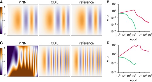
Poisson equation solved using PINN and ODIL. The exact reference solution is an oscillatory function  and ODIL with Adam
  compared to the exact reference solution for
Velocity from tracer
We consider the evolution of a tracer field governed by the advection equation in two dimensions. The problem is to find a velocity field
in a unit domain, and the initial
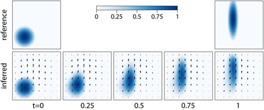
Inferring the velocity field from two snapshots of a tracer. The tracer satisfies the advection equation with an unknown velocity, and the reference tracer is imposed at the first and final time instants. Arrows show the inferred velocity field.
Inferring the velocity field from tracers is an example of the optical flow problem (11) in computer vision and the image registration problem (63) in medical imaging. Furthermore, reconstructing the velocity field from a concentration field can assist experimental measurements.
Inferring conductivity from temperature
Here, we consider an inverse problem of inferring a conductivity function from temperature measurements. We solve the problem in a unit domain
with zero Dirichlet boundary conditions
for
using second-order extrapolation. The loss function for the inverse problem consists of the residual and terms to impose the temperature measurements
where
where
To generate the temperature measurements and the reference solution, we specify the reference conductivity function as
and solve the forward problem using ODIL on a grid of
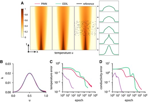
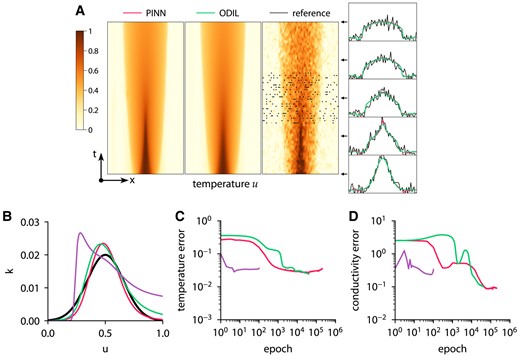
Inferring conductivity from temperature measurements using ODIL and PINN. Temperature field (A) and conductivity function (B) inferred by PINN with Adam , ODIL with Adam , and ODIL with Newton  compared to reference
  . The reference solution is from forward problem solved using ODIL on a finer grid. The temperature measurements in 200 points (black dots) are taken from the reference solution. History of root-mean-square error in temperature (C) and conductivity (D).
Inferring conductivity from noisy temperature measurements using ODIL and PINN. Temperature field (A) and conductivity function (B) inferred by PINN with Adam , ODIL with Adam , and ODIL with Newton compared to reference . The reference solution is from forward problem solved using ODIL on a finer grid. The temperature measurements in 200 points (black dots) are taken from the reference solution perturbed by Gaussian noise with
Lid-driven cavity: forward problem
The lid-driven cavity problem is a standard test case (64) for numerical methods for the steady-state Navier–Stokes equations in two dimensions
where
Figure 6 shows the streamlines for values of
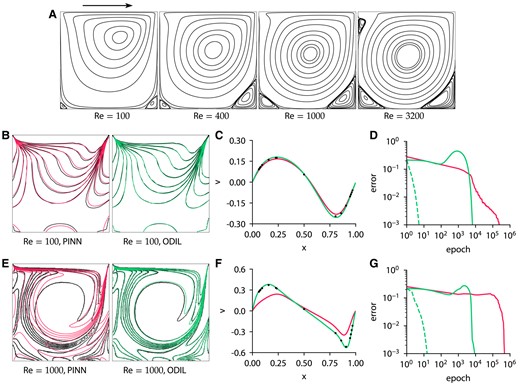
Lid-driven cavity problem solved using PINN and ODIL. A) Streamlines for and ODIL with Newton . E–G) Same for . Reprinted with permission from Elsevier. C, F) Profiles of velocity v along the centerline  . D, G) History of root-mean-square error in velocity u obtained using PINN with L-BFGS-B , ODIL with Newton
  , and ODIL with Adam . The error of PINN is relative to the solution after 500,000 epochs with L-BFGS-B. The error of ODIL is relative to the solution after 100 epochs with Newton.
Lid-driven cavity: flow reconstruction
Here, we solve the same equations [34] as in the forward problem, but we impose the known velocity values
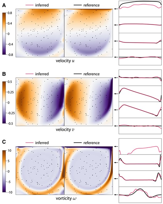
Lid-driven cavity flow at
Measure of flow complexity
Based on the flow reconstruction from velocity measurements using ODIL in the previous case, we introduce a measure of flow complexity. Consider a velocity field
where
To illustrate this complexity measure, we consider four types of flow: uniform velocity, Couette flow (linear profile), Poiseuille flow (parabolic profile), and the flow in a lid-driven cavity. The reference velocity fields in the first three cases are chosen once at an arbitrary orientation and such that the maximum velocity magnitude is unity. As in the previous case, we do not impose any boundary conditions for the velocity, replacing them with linear extrapolation. However, to generate the samples faster, we use a smaller
with

Fluid flow reconstruction error depending on the number of measurement points for various flows: uniform, Couette flow, Poiseuille flow, and lid-driven cavity. The dots show samples of random sets of K points and the minimum over them is an estimate of the minimal reconstruction error .
Inferring body shape from velocity in two dimensions
Here, we consider a 2D inverse problem of inferring the shape of a body from measurements of the flow velocity around the body. The model consists of the steady-state Navier–Stokes equations with penalization terms to impose the no-slip conditions on the body (67)
where λ is a penalization parameter and D is a characteristic length of the body. The shape of the body is described by the body fraction
To solve the inverse problem using ODIL, we formulate it as minimization of the loss function in terms of the unknown fields: velocities u and v, pressure p, and a level-set function
discretized using an upwind scheme (68). The parameter decays as
This approach with the level-set function ensures that the interface is diffused over a constant number of cells. The reference data are obtained from the forward problem. The chosen grid is sufficiently fine to resolve the flow based on the grid refinement study in Fig. S11. Figures 9–11 show the results of inference for three different bodies: a circle, an ellipse, and a nonconvex body. The characteristic length of the body is
describing a small circle. The optimization takes 20,000 iterations and completes in about 3 min on one CPU core. ODIL recovers the reference shape from velocity measurements in 100 points if the shape is convex. However, we observe that the method does not infer nonconvex shapes and instead finds a convex shape that matches the velocity measurements.
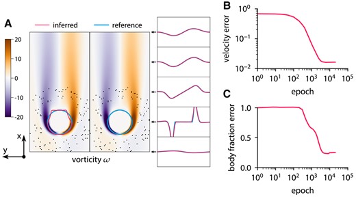
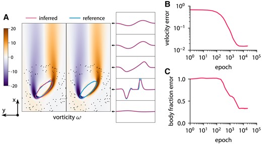
Inferring body shape from velocity measurements for a flow past a circle at and reference  vorticity ω overlapped by contours of body fraction
Inferring body shape from velocity measurements for a flow past an ellipse at and reference vorticity ω overlapped by contours of body fraction
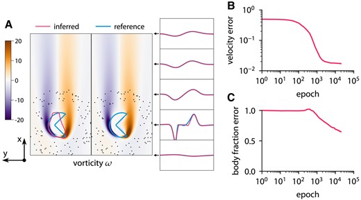
Inferring body shape from velocity measurements for a flow past a nonconvex body at and reference vorticity ω overlapped by contours of body fraction
Inferring body shape from velocity in three dimensions
Here, we consider a 3D inverse problem of inferring the shape of a body from measurements of the flow velocity around the body. The model consists of the steady-state Navier–Stokes equations with penalization terms to impose the no-slip conditions on the body (67)
where λ is a penalization parameter and D is a characteristic length of the body. The shape of the body is described by the body fraction
To solve the inverse problem using ODIL, we formulate it as minimization of the loss function in terms of the unknown fields: velocity
Figures 12 and 13 show the results of the inference from 684 measurement points for two different bodies: a sphere and a hemisphere. The convergence history includes the velocity error and the body fraction error which are defined relative to the solution of the forward problem. In both cases, ODIL recovers a body shape that qualitatively agrees with the reference, although the relative error in the body fraction field amounts to 50%, so the inferred body volume is larger. On a GPU Nvidia A100, the forward problem with a sphere takes 53 min in total and
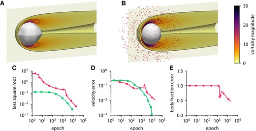
Inferring body shape from velocity measurements for a flow past a sphere using ODIL. A, B) Inferred (A) and reference (B) body shape and contours of vorticity magnitude. The velocity measurements are imposed in 684 points (red dots) chosen at a distance from the body. C–E) History of the square root of the loss (C), root-mean-square error in x-velocity (D), and body fraction χ normalized by the mean of reference (E) for the inverse problem  and forward problem
  . The error is relative to the solution of the forward problem after 10,000 epochs.
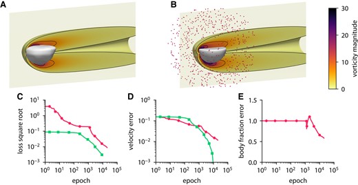
Inferring body shape from velocity measurements for a flow past a hemisphere using ODIL. A, B) Inferred (A) and reference (B) body shape and contours of vorticity magnitude. The velocity measurements are imposed in 684 points (red dots) chosen at a distance from the body. C–E) History of the square root of the loss (C), root-mean-square error in x-velocity (D), and body fraction χ normalized by the mean of reference (E) for the inverse problem and forward problem . The error is relative to the solution of the forward problem after 10,000 epochs.
Conclusion
We introduce the ODIL framework for solving inverse problems for PDEs by casting their discretization as an optimization problem and applying optimization techniques that are widely available in machine-learning software. The concept of casting the PDE as is closely related to the neural network formulations proposed by (15–17) and recently revived as PINNs. However, the fact that we use the discrete approximation of the equations allows for ODIL to be orders of magnitude more efficient in terms of computational cost and accuracy compared to the PINN for which complex flow problems “remain elusive” (71).
We remark that the error of PINN typically scales as a square root of the number of training points regardless of the space dimensionality (25), which can be beneficial for high-dimensional problems (72, 73). However, a recent attempt (36) to apply PINN for simulating an open quantum system has proven unsuccessful, outperformed by the Q-Flow method based on normalizing flows proposed therein. In ODIL, the grid-based discretization may suffer from the curse of dimensionality as the error of a p-order accurate method with N grid points scales as
We have presented the applications of ODIL to several forward and inverse problems involving PDEs, including the Poisson equation, the heat equation, the advection equation, and the Navier–Stokes equations. In most cases, the discrete loss has been formulated using second-order accurate finite volume discretizations and incorporate exactly the boundary and initial conditions through extrapolation. We emphasize that the primary scope of ODIL is in solving ill-posed and inverse problems. For forward, and in particular time-dependent problems, a multitude of classical solvers based on marching in time are far more efficient than PINNs and ODIL since they do not require storing all the time steps as unknowns.
The ideas and results presented in this article suggest that ODIL, and even more the ideas it entails, can serve as inspiration for advancing the solution of inverse problems. We remark that while ODIL is shown to vastly outperform PINNs, its development was motivated by the widespread use of PINNs and their treatment of equations and data. We believe that there are many promising venues at such interfaces (and competitions) of machine learning and scientific computing for solving inverse problems using physics and data informed methodologies. Ongoing works using ODIL include tracking the evolution of brain tumors from medical images (78), the derivation of material properties for specific heat conduction and the identification of submerged obstacles from surface information.
Acknowledgments
The authors thank Professors Michael P. Brenner (Harvard University), Georges-Henri Cottet (retired), and Thomas Y. Hou (Caltech) for several insightful discussions. They are also grateful to the five anonymous Reviewers for their multiple, valuable suggestions that helped us to improve this article.
Supplementary Material
Supplementary material is available at PNAS Nexus online.
Funding
This work was supported in part by funds from The European High Performance Computing Joint Undertaking (EuroHPC) Grant DCoMEX (956201-H2020-JTI-EuroHPC-2019-1). P.Ko. acknowledges support by the AFOSR program (FA9550-21-1-0058).
Author Contributions
P.Ka.: methodology, software implementation of ODIL, visualization, and writing (original draft). S.L.: methodology, software implementation of PINN, validation, and writing (review and editing). P.Ko.: conceptualization, methodology, supervision, and writing (review and editing).
Preprints
A preprint of this article is published at arXiv:2205.04611.
Data Availability
The source code of the implementation of the method is available at https://github.com/cselab/odil along with examples and instructions to reproduce the results.
References
Author notes
Competing Interest: The authors declare no competing interest.