


Abstract
Quantitative understanding of the process of knowledge creation is crucial for accelerating the advance of science. Recent years have witnessed a great effort to address this issue by studying the publication data of scientific journals, leading to a variety of surprising discoveries at both individual level and disciplinary level. However, before scientific journals appeared on a large scale and became the mainstream for publishing research results, there are also intellectual achievements that have changed the world, which have usually become classic and are now referred to as the great ideas of great people. So far, little is known about the general law of their birth. In this paper, we reference Wikipedia and academic history books to collect 2001 magnum opuses as representations of great ideas, covering nine disciplines. Using the year and place of publication of these magnum opuses, we show that the birth of great ideas is very concentrated in geography, and more concentrated than other human activities such as contemporary knowledge production. We construct a spatial–temporal bipartite network to study the similarity of output structures between different historical periods and discover the existence of a Great Transformation around the 1870s, which may be associated with the rise of the US in academia. Finally, we re-rank cities and historical periods by employing an iterative approach to study cities’ leadership and historical periods’ prosperity.
We collect metadata of 2001 magnum opuses written by notable people to analyze the spatial–temporal patterns of the birth of great ideas. We characterize precisely the geographic concentration of great ideas and their evolution over time. We construct a spatial–temporal bipartite network to study the similarity of output structures between different historical periods and discover a Great Transformation in academia around the 1870s. Our research shows that social factors play a non-negligible role in when and where great ideas arise; great ideas in the humanities, social sciences, and natural sciences follow the same spatial–temporal patterns. Besides, we re-rank cities and historical periods by measuring cities’ leadership and decades’ prosperity.
Introduction
Since de Solla Price discovered the exponential growth law of scientific literature (1), the quantitative study of scientific practice has been an active research field. Scientometrics has made much effort in evaluating scientific impact, analyzing citation relationships, and visualizing science (2). In recent years, broader research on science practice has begun to integrate research methods from fields such as machine learning, network science, and economics, with surprising results on expanded topics including scientific teamwork (3–6), research-interest evolution (7–9), and individual scientists’ careers (10–13), among others. This emerging interdisciplinary study is called the science of science (14, 15). At the same time, scientific activity is regarded as a process of knowledge production and innovation. Its imbalanced geographical distribution (16–20) and its relationship with other regional variables (21–23) have been extensively studied in spatial scientometrics and economic geography, with an important role in guiding the development of regional innovation policy.
These data-driven studies rely heavily on scientific literature databases. Since the digitization of scientific literature started much later than the entire scientific development process, most of the time periods covered by the available data in these databases only start at the late 19th or 20th century (14, 24, 25). This also results in quantitative research on the laws of scientific activities covering only a limited historical period. Before that, humans actually have produced a large number of important intellectual achievements. From Newton’s Mathematical Principles of Natural Philosophy, the progressive political thought of the Enlightenment, Kant’s critical philosophy, Darwin’s theory of evolution, Freudian psychoanalysis, to the Keynesian revolution, the striking feature of the last few centuries is the continued emergence of great ideas. Whether they were mathematicians, scientists, philosophers, economists, or politicians, these great people have brought us great ideas that have profoundly changed the world. The study on great ideas is imperative, but surprisingly, apart from qualitative studies of these great ideas from the perspectives of academic history and intellectual history (26, 27), quantitative studies have been missing. Therefore, we ask: What are the general laws for the production of great ideas? What are the similarities and differences between these general laws and those of contemporary paper-based scientific practice?
Great thinkers are gone, long live ideas. Publications of notable people printed, published, and circulated in cities are just the external representation of great intellectual achievements. These magnum opuses written by notable people contained their most profound, wise, and subversive intellectual achievements, which continue to exert their influence today, especially books—they are primary carriers for great ideas. Thus, we extract 2001 magnum opuses from Wikipedia and academic history books in nine disciplines: mathematics, physics, chemistry, biology, philosophy, economics, politics, sociology, and psychology. We collect bibliographic metadata including the year of publication and the place of publication. Using them, we examine the geographic concentration of great ideas and the evolution of concentration over time. The results show that the output of great ideas is more spatially concentrated than human activity in general. We construct a spatial–temporal bipartite network to study the similarity of output structures between different decades. Most notably, a universal pattern of temporal characteristics across disciplines is found, which may be associated with the rise of the US in academia. Finally, we design an iterative algorithm to re-rank the cities and historical periods that produced great ideas and find that some cities with high output were unable to maintain long-term advantages, reflecting the difference between organized professional science and amateur pattern relying on the Zeitgeist.
Results
Our goal is to represent the intellectual achievements in nine disciplines ranging from Newton’s Mathematical Principles of Natural Philosophy (1687) to Philosophical Investigations (1953) by Wittgenstein. Unlike bibliographic data science (28, 29), these publications we collected are only classic works in their fields or representative works of notable people who have made outstanding contributions in these nine disciplines during these 267 years and are therefore of cultural importance. We collect data by the process shown in Fig. 1. Table 1 is the basic statistics of the 2001 publications written by 1168 authors (including coauthors). We collected the author name(s), year of publication, and place of publication of all these publications, which contains 129 cities in total. We use these places to locate great ideas. All of these cities are located in Europe or the US.
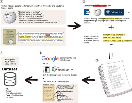
Data collection process. Step 1: Reference Wikipedia and books on academic history in nine disciplines, and collect notable people and their magnum opuses. Step 2: Search for notable people in the encyclopedia websites, and further identify their representative works through biographies. Step 3: Combine the magnum opuses collected in Step 2 and Step 1 to form a book list (or, to be precise, a publication list). Step4 : Google every title in the book list to find bibliographic metadata for these books. For the metadata of the paper, see Supplementary Material, section 6. Step 5: Establish a dataset, which contains the title, author, year of publication, place of publication, and other information of all 2001 magnum opuses. For a more detailed explanation of data collection, see Materials and methods.
Basic statistics of data.
| Discipline | Number of worksa | Number of authorsb | Number of cities |
|---|---|---|---|
| Physics | 350(61) | 220 | 46 |
| Philosophy | 313(5) | 173 | 54 |
| Mathematics | 290(48) | 194 | 48 |
| Economics | 234(3) | 153 | 48 |
| Biology | 197(16) | 128 | 40 |
| Chemistry | 179(13) | 127 | 38 |
| Psychology | 174(1) | 94 | 26 |
| Politics | 135(2) | 101 | 34 |
| Sociology | 129(1) | 96 | 31 |
| Total | 2001(150) | 1168 | 129 |
We prioritize the use of a person’s books as representations of his or her ideas. But there are some important ideas whose creators did not use books to present them, in which case we use papers instead. Therefore, the 2001 works are not all books but contain also 150 papers. The numbers in parentheses in the second column indicate the number of papers in the works of the corresponding discipline.
The total number of authors is less than the number of authors for the nine disciplines combined, because some authors span multiple disciplines. So does the number of cities.
Geographic concentration
Related research on knowledge production has shown that paper-based contemporary knowledge production has the place-dependent character (30–32), that is, papers are more likely to be produced where papers have already been produced. The data we collect have similar characteristics. Fig. 2A shows the top 40 cities in terms of publication output. The output of the top five cities accounted for more than half of the total output—London, Paris, New York, Leipzig, and Berlin published a total of 1176 out of 2001 works. Fig. 2B shows that the number of works and the number of locations follow Heaps’ law, i.e. . The smaller the exponent, the more likely the works are to appear in locations that already exist. The sublinear exponent of overall indicates that when the number of works becomes 10 times as many as before, the number of locations only becomes (about 4.37) times as many as before. There are differences in the exponents for different disciplines (see Supplementary Material Figure S1), but they are all less than 1. Fig. 2C shows the complementary cumulative probability of the city’s publications output in nine disciplines. In logarithmic coordinates, they are straight lines sloping downward, which also implies that the publications output by cities seems to follow Zipf’s law (see Supplementary Material Figure S2). It shows the heterogeneity in early knowledge production, which is also a sign for geographic concentration.
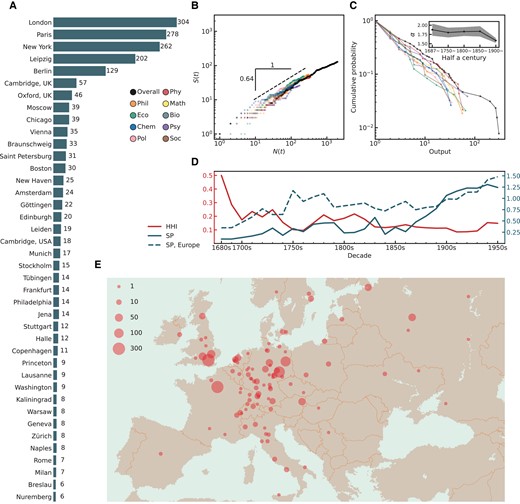
Geographic concentration of great ideas. A) Histogram of publications output for the top 40 cities. B) The number of works as a function of the number of locations , where the exponent of overall . See Supplementary Material Figure S1 for separate exponents for each discipline. C) Cumulative probability distribution for publication frequency in locations, by disciplines. In the inset, we divide the time span into five parts: 1687–1749, 1750–1799, 1800–1849, 1850–1899, and 1900–1953. We show the power-law exponent of the distribution of publication frequency within each period. The power-law exponent is calculated with an established method by Aaron Clauset et al. (33) The shaded area indicates the confidence interval. D) The evolution of concentration. We show changes over time in HHI, which reflects the degree of concentration, and SP, which reflects the degree of spatial separation. In general, HHI decreased over time with the diffusion of knowledge from London, and SP increased over time with the rise of the US in later periods. In the 1910s, the HHI reached its lowest value, 0.085. E) Map of publications output, European region. In 1954, J. D. Bernal drew a map titled “Scientific and Industrial Europe” in his monumental work Science in History, describing the distribution of scientific and industrial centers in Europe from the 18th to the 20th century to illustrate that the distribution of science and industry closely corresponded (34). Here, similarly, we draw the distribution of the output of great ideas in Europe, measured by magnum opuses. The size of the point scale with the square root of the city’s output. See Supplementary Material Figure S3 for the map of the US.
Based on the above analysis, we can say that the production of great ideas has a spatial characteristic of geographic concentration. We further observe changes in concentration through the Herfindahl–Hirschman Index (HHI) and the Spatial Separation Index (SP) (see Materials and methods for details). The closer HHI is to 1, the greater output concentrates in fewer cities. HHI is an index that does not consider the distance between cities, so SP is used as a complement to HHI. The higher the SP, the more spatially dispersed academic publishing is. The red line in Fig. 2D indicates HHI, the gray-blue line indicates SP. The HHI was high in the 1680s and 1690s when the production of publications was still disproportionately concentrated in London, and its influence continued into the 1740s. At the same time, knowledge spread to the European continent (SP rising) constantly. Subsequently, the two indices fluctuated in small ranges during 100 years. In the 1870s, things began to change. It can be seen that although two historical periods—from the 1750s to the 1760s and from the 1870s to the 1930s—had similar HHI, their SP were quite different. It is because of the rise of the US in academia, which first started with sociology and psychology, then economics, politics, and philosophy. By the 1940s, the US had its places in almost every discipline. As the US is far away from Europe, this change led to a constant increase in SP. Over the same period, the degree of concentration was slowly declining. Therefore, these two indices show the process about how knowledge spillover in Britain in the early years and the headlong rise of the US in the later years.
We further ask whether the rise in SP after the 1870s is only because of the US? And whether academic research in Europe was also in a state of separation during this period? The gray-blue dashed line in Fig. 2D indicates the SP calculated only for the European region, which can help us investigate the changes in Europe. After the influence of the UK waned, the SP reached a 40-year high point from the 1750s to the 1780s. During this period, the Enlightenment was at its peak. The Encyclopedia School began to publish the famous Encyclopédie from 1751; Chemical and biological works continued to appear in northern Europe; Italian economists took their place in the history of economics; The great mathematician Euler returned from Berlin to Saint Petersburg; As the end of this climax, Kant emerged in Königsberg (Kaliningrad), and his book was published in distant Riga. These places are scattered across Europe, resulting in high SP. The second rise of SP in Europe came after the 1870s, although we have excluded the influence of the US. It was slowly climbing as well, approaching the levels of the 1750s in the 1920s and 1930s, and then climbing further. This was a period of great development for many countries in Europe, for the Second Industrial Revolution brought out a rapid increase in productivity. Croce called the period from 1870 to 1914 (when World War I broke out) the era of freedom (35), which has also been referred to by others as the first globalization period. These social factors have all contributed to the continued increase of SP in Europe.
Finally, we compare the degree of the concentration of great ideas with other human activities. Spatial concentration is an important feature of human activity. It first manifested as human beings live and work in cities. In 1949, Zipf studied the city size distribution and believed that it can be approximated by the Pareto distribution with a parameter equal to 1 (36, 37). Subsequent studies have shown that the parameter is actually on average significantly larger than 1 from 1500 (38–40). In contrast, the generation of great ideas has a lower parameter. Fig. 2C illustrates that the output of great ideas also follows a Pareto distribution, with calculations showing parameters ranging from 0.5 to 1 for individual disciplines and overall. The inset in Fig. 2C shows the parameter changes by time period (for the overall). Shown on the inset is the exponent of the power law, whose value minus one is the parameter of the corresponding Pareto distribution. The inset implies that the parameters of the Pareto distribution for different time periods are all less than 1. On the other hand, we compare the HHI of great ideas and city size over the time period we consider. Using a new dataset of European urban populations (41), we calculate the HHI of city size spanning the period 1700–1950 in steps of half a century. For a reasonable comparison, we recalculate the HHI using the great ideas belonging to Europe in our data. As shown in Supplementary Material Figure S21, great ideas’ HHI is substantially higher than the city size’ HHI. All this shows that great ideas are more concentrated than the city size during the time period we consider.
Contemporary knowledge production is another comparable human activity. Spatial Scientometrics shows that scientific research activities were disproportionally concentrated in a small number of countries (16–19). The results of regional innovation are similar, and one of the reasons behind them is believed to be the existence of tacit knowledge (42). In Polanyi’s view, the art of science, like the art of craftsmen, relies on localized master-apprentice teaching to pass on tacit knowledge (43). Here, we use the study by Mu-Hsuan Huang et al. as a comparison, which is about the trend of global concentration in scientific research and technological innovation from 1981 to 2008 (20). The study showed that the HHI value on the production of paper (in the country level) remains between 0.1 and 0.2 during this period. We recalculated the HHI in the country level, which is generally higher than 0.2, as shown in Supplementary Material Figure S22. This suggests that the production of great ideas is generally more concentrated than the production of contemporary papers.
Output structure and academic development path
For different historical periods, the output of publications in different cities accounts for different shares of the total output, and we call this the output structure. Changes of the output structure in different periods can help us observe the history of academic development. We analyze this by constructing a spatial–temporal bipartite network with time: One type of nodes in this bipartite network represent cities and the other type of nodes represent time periods. Therefore, unlike the region-subfields network (32, 44), our network itself contains temporal information. We group time by decade, so a time period node represents 10 years. Further, we use an approach similar to generating the product space (45) to obtain a similarity network of the output structure of the decades, which we call “decade space.” In the decade space, decade nodes with more similar output structures have higher proximity and thus are connected. See Materials and methods for the detailed construction process of the network.
As an example, Fig. 3A shows the decade space of philosophy. It can be found that the decade nodes that are closer in time are also closer in decade space as a whole. The nodes from the 1680s to the 1750s are clustered in the upper left of the decade space, and the decade nodes representing the time closer to the present are closer to the right. This shows that the development of philosophy as a whole is a gradual change. Despite this, there are a small number of node pairs that are connected to each other and represent decades far apart, which means the existence of long-range correlations. For example, in philosophy, the 1800s are only connected to the 1910s; the 1950s are connected with the 1830s and 1850s. This kind of long-range correlation appears in various disciplines (see Supplementary Material Figures S5–S12), and its significance is related to the details of specific academic history. Technically speaking, the node pair has a long-term correlation because they have more common cities which have comparative advantages in both decades. Therefore, we mark the decades that the top cities in terms of publication output have comparative advantages in with colors to observe the impact of these cities on the structure of the decade space. Fig. 3B–D shows, respectively, the decades that London, Leipzig&Berlin, and New York have comparative advantages in (the nodes with color marking). We can see that the comparative advantage of Leipzig or Berlin contributed to the connection between the 1800s and the 1910s, and the comparative advantage of London contributed to the connection between the 1950s and the other two decade nodes. This suggests that the renaissance of cities in academic history is the reason for the long-term correlation.

An example of the decade space. A) The decade space of philosophy. We use Gephi to generate the network with Force Atlas layout. The size of each decade node scales with the output of publications in that decade. The width of an edge scales with the proximity between two nodes. Here, the different colors of the edges are just to distinguish different edges. In general, decade nodes that are close to each other in time are located close to each other and more tightly connected in the decade space. The nodes from the 1680s to the 1750s are clustered in the upper left area of the decade space, and the farther to the right, the closer the decade node is to the present. The node of the 1800s, however, is an exception. The output structure of the 1800s (Herbart in Göttingen, Hegel in Bamberg) is not very similar to any other decades, it is linked to the 1910s by the comparative advantage of Berlin and Tübingen (Schelling’s System of Transcendental Idealism and Husserl’s Philosophy as Rigorous Science) (proximity 0.22). B–D) The decades that London, Leipzig&Berlin, and New York have comparative advantages in are color-marked. We can see that the decades that a certain city has comparative advantages in are close. The emergence of London is a reason why the output structure in the 1950s was closer to that of a century earlier.
Furthermore, we can find that the decades that different cities have comparative advantages in are quite different, and they occupy different positions in the decade space. This reflects the rising progress of different cities in the history of philosophy and how these cities influenced the path of philosophy’s development. London’s comparative advantages (Fig. 3B) from the 1680s to the 1770s reflected the development of British empiricism and the philosophy of the Scottish Enlightenment (some of the monumental works of the Scottish Enlightenment were published in Edinburgh, while some in London). But then the continued popularity of Deism eventually hindered the further development of British philosophy. The 1780s and 1790s were another beginning (Fig. 3C), and from Kant, Fichte, Schleiermacher, Schelling, Hegel, Schopenhauer, Feuerbach, to Nietzsche, German philosophy gave out another path in decade space—the advantage extended upwards from the lower left section, and finally converged in the 1870s. The output structure in the 1870s not only inherited the past but also determined the future (see The Great Transformation around the 1870s for a detailed discussion). Therefore, publications from Leipzig and Berlin dominated the output structure for a period after the 1870s. Another force that emerged from the 1890s to the 1940s was American pragmatism (Fig. 3D). It is representative of American philosophy in the first half of the 20th century, and due to its late appearance, it occupies the right position in the decade space.
The phenomenon that different cities occupy different positions in decade space also occurs in other disciplines (similar analyses in other disciplines are presented in Supplementary Material Figures S5–S12). This shows that the academic center with dominant position of each discipline has continued to shift with historical development. In this regard, sociology of science and geographies of science had put forward a similar point of view—from the 17th century to the 20th century, the scientific center was constantly shifting from the UK, France, Germany, and finally to the US (46, 47). Our results show that this shift occurs not only in natural sciences, but also in social sciences (economics, politics, psychology, and sociology) and humanities (philosophy).
The great transformation around the 1870s
Across different disciplines, we focus on the consistency of the output structure of decade spaces. If such consistency exists, it means that there is a stable pattern in different disciplines’ academic development history.
Fig. 4A–I shows the decade space of all nine disciplines, where Fig. 4A–F represents physics, philosophy, mathematics, economics, biology, and politics. These six decade spaces all can be divided into two parts—the left part contains earlier decades, while the right part contains later decades. This shape looks like an hourglass laid horizontally, so we call this hourglass-shaped structure. It means that they all have more similar output structures in the decades before a certain decade, and so do in the decades after the certain decade, but the proximity of the output structure between the two parts is very low. Moreover, these “certain decade” in the different decade spaces, as the dividing line in time, have much in common. In Fig. 4J, we marked these nodes in the six decade spaces, which happen to be the nodes with the largest or the second largest betweenness centrality in each decade space. More importantly, most of these nodes denote periods around the 1870s. Therefore, it is reasonable to consider that these six disciplines share the same pattern. More specifically, around the 1870s, the world of academic research changed dramatically, and the world before it was markedly different from the world after it. To the best of our knowledge, little has ever observed this phenomenon before. We call this the Great Transformation around the 1870s.
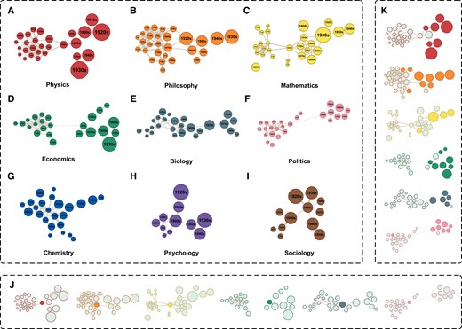
The Great Transformation around the 1870s. A–G) The decade space of physics, philosophy, mathematics, economics, biology, politics, and chemistry. These decade spaces show an hourglass-shaped structure, except for chemistry. H and I) show the decade space of psychology and sociology, respectively. Since these two disciplines appeared late, the decade spaces of them are not able to form the hourglass-shaped structure. J) The nodes with the largest or second largest betweenness centrality in the first six decade space are color-marked. Except for mathematics, these “bridge nodes” all belong to the period around the 1870s: the 1880s for physics, the 1870s for philosophy, the 1870s for economics, the 1860s for biology, and the 1860s for politics. Mathematics also has an hourglass-shaped structure, but its “bridge node” appeared in the 1830s, just after the most prosperous decade in mathematics. K) We mark the decades that the top three US cities in that discipline’s publication output have comparative advantages in with colors. The color-marked nodes are all located in the right group that representing the post-1870s.
We further move to understand the reason behind this phenomenon. One possible explanation is the rise of the US in academia. After the Civil War, the US entered the Gilded Age and the Progressive Era. The rapid growth of economic and other developments provide the possibility for the emergence of professional academic researchers. Fig. 4K shows the rise of America in academia after the 1870s. The decades that the top three US cities in that discipline’s publication output have comparative advantages in every discipline’s decade space are color-marked. It is clear that the US mainly has comparative advantages in the decades after the Great Transformation instead of before it. This obviously increases the proximity between the decades after the Great Transformation and decreases the proximity between the two decade groups before and after the Great Transformation. In addition to the reasons for the US, this Great Transformation of decade space may also have other more complex historical contexts, which need to be further studied.
City’s leadership and decade’s prosperity
We can see in previous sections that some cities, such as London, Paris, New York, Leipzig, and Berlin, tend to have decades of dominance in many disciplines. As academic centers with leadership, they lead the development of the discipline. How to rank for this long-term advantage of them? We believe it is biased to consider it solely in terms of output. We design an iterative method on the spatial–temporal bipartite network to help us achieve this goal, and it can measure city’s leadership and decade’s prosperity . For each iteration, the city’s leadership is positively related to the prosperity of the decade to which it is connected, while the decade’s prosperity is nonlinearly related to the leadership of the city to which it is connected. After many iterations, the and will stabilize, resulting in a final result (see Materials and methods). High leadership means that the city has advantages in many prosperous decades. High prosperity means that the decade is in a situation where a large number of small cities were productive and different cities prospered and developed together in academic history.
Fig. 5 shows an example of the comparison of the publications output ranking and our iterative results (leadership or prosperity ranking). It is about mathematics and Supplementary Material Figures S13–S20 provide the comparison of rankings in all other disciplines. According to Fig. 5B, although Paris ranks first in mathematical publications output, it ranks fifth in leadership. This is because the publications published in Paris were concentrated in the early 19th century. At that time, the École Polytechnique and École normale supérieure trained a large number of well-known figures, especially mathematicians (48). Unlike Paris, which lacked leadership in many other decades, Berlin ranks third in publications output and first in leadership. This shows the influence of the Berlin school—a group of German mathematicians represented by Weierstrass gathered in Berlin to study mathematics in the second half of the 19th century.
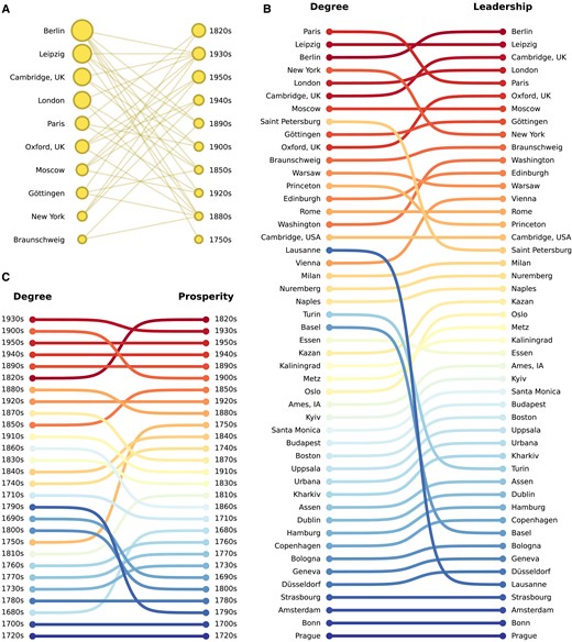
Comparison between degree and our new results, in mathematics. A) The bipartite network of the top 10 cities for leadership and the top 10 decades for prosperity. Node size scales with leadership or prosperity. B) City’s degree (i.e. the publications output of the city) vs. city’s leadership. Colors are assigned by the leadership ranking. C) Decade’s degree (i.e. the publications output of the decade) vs. decade’s prosperity. Colors are assigned by the prosperity ranking.
The imbalance in Paris in terms of leadership and publications output is not only reflected in mathematics. Although Paris ranks second overall in output (see Fig. 2A) and tops in every discipline, its leadership ranking compared to its output ranking decreases in varying degrees in six disciplines (see Supplementary Material Figures S13–20). This is also because France’s output is too concentrated on certain times in its history. Before and after the French Revolution, rising scientific enthusiasm led Paris to become the academic center of the world. This caused the high state of HHI during this period (see Fig. 2D). But the institutionalization of science caused France to decline rapidly, after which Germany immediately overshadowed the brilliance of France (see Supplementary Material Figure S4). These show that in the process of the emergence of great ideas, some regions systematically produce great ideas by organized professional science, thus maintaining a long-term advantage, while others like Paris are fleeting, that is only the ephemeral product of a Zeitgeist (49).
As shown in Fig. 5C, according to our calculations, the 1820s is the most prosperous decade in the history of mathematics, although it ranks sixth in publications output. During this period, Paris’ dominance of mathematics was drawing its end (Cauchy, Poncelet, Fourier, and Legendre), Gauss was doing his research in solitude in Göttingen, and Dirichlet published his famous article on Fourier series in Berlin. The dissemination of knowledge also bore fruits in other parts of the Continent—Jacobi in Königsberg (Kaliningrad) published New Foundations of the Theory of Elliptic Functions (1829); Abel, a frustrated contributor, published the famous Memoir on algebraic equations, in which the impossibility of solving the general equation of the fifth degree is proven (1824) in Oslo at his own expense; Lobachevsky pioneered non-Euclidean geometry in distant Kazan (1829).
Our algorithm successfully reveals this boom, and it is also effective in other disciplines. In addition to mathematics, the most prosperous decades for other disciplines were concentrated in the interwar years—the 1920s for biology, psychology, and sociology, and the 1930s for philosophy, economics, and politics. The most prosperous decades in physics and chemistry were in the 1940s, but their subprosperous decades were not much different from their most prosperous decades (for physics, the of the 1940s and the 1920s are 2.03 and 2.01, respectively; for chemistry, the of the 1940s and the 1920s are 1.76 and 1.72, respectively). Therefore, it can be argued that the interwar period was the most prosperous period of academic development in the time span of our data. During this period, many countries that were originally in a marginal position ushered in rapid academic development, such as psychoanalysis and logic in Vienna, mathematics in Eastern Europe, and the Swedish school in economics. And the Soviets also started to make their marks in mathematics, physics, biology, and psychology during this period.
Conclusion
We collect 2001 academic magnum opuses using Wikipedia and academic history books and study the spatial–temporal patterns in the generation of great ideas on this new dataset. It can be found that, on the whole, the production of great ideas is very concentrated in geography, and more concentrated than other human activities such as contemporary knowledge production. And within our time-window, this kind of concentration has gradually diminished. We construct a decade space to study the similarities in the output structure of great ideas of different historical periods. In the decade space, the decades that are close to each other in time are also closer in the network, and the decades that different cities have comparative advantages in clearly show the academic development paths and the shift of academic center. Six of the nine disciplines’ decade spaces exhibit the same pattern—an hourglass-shaped structure, which indicates the existence of the Great Transformation in academia around the 1870s. Finally, we re-ranked cities and decades to identify the highest leadership cities and the most prosperous decades for each discipline.
Our results quantitatively support some of the views in history of science and sociology of science and extend them to the humanities and social sciences. First, the early sociology of science has always been concerned with the relationship between the production of scientific knowledge and social factors (46, 50, 51). More specifically, people study the social construction (52, 53), linguistic context (54), spatial factor (55), etc. behind great ideas. The sociology of scientific knowledge (SSK), which emerged in the 1970s, further claims that the content of scientific knowledge itself is constructed by society, emphasizing that scientific research as a human social activity will be affected by social conditions (52, 53, 56, 57). This claim has caused quite a bit of controversy in the scientific community. And such arguments, known as social constructionism, also hold that not only scientific knowledge, but all knowledge in everyday reality, including commonsense knowledge, is socially constructed (58). In this paper, we found that great ideas exhibit geographic concentration, shifts of center, and the presence of the Great Transformation. These characteristics are considered by us to be related to social context. We therefore come to an important conclusion that social construction plays a non-negligible role in the generative form of great ideas. Although great ideas do not contain all knowledge, our results are still representative. Note that our results only imply social construction on the form (i.e. spatial–temporal patterns), not content, because our data have no bearing on the content of great ideas.
Second, unlike the sociology of science or SSK described above, we are concerned not only with the natural sciences but also with the humanities and social sciences. Economics, politics, and philosophy all have similar characteristics to natural sciences such as mathematics, physics, and biology, both in terms of geographic concentration and shift of academic center. The hourglass-shaped structure of the decade space also shows that the humanities and social sciences follow a pattern similar to that of the natural sciences. In a word, there is not much difference between the ideas of humanities and social sciences and that of natural science in terms of the spatial–temporal characteristics. Our research deserves the attention of researchers in the sociology of science, those in the history of the natural sciences, those in the history of the humanities and social sciences, and anyone else interested in the progress of human reason and intellect over the past few centuries. Third, compared to contemporary knowledge production based on papers, the generation of great ideas also has the phenomenon of geographic concentration, but a shift in the center of concentration can be observed over a larger time span. Our results demonstrate how the US has gradually achieved the position it holds today, and this influences the spatial–temporal pattern of the output of great ideas.
We note several limitations of our research. Our data lack some disciplines such as earth science, jurisprudence, and history to provide more complete support for our conclusions. Another limitation is about the interpretation of the results: Why chemistry does not exhibit an hourglass-shaped structure in decade space remains to be further investigated; we already know the impact of the rise of the US on the spatial–temporal patterns of great ideas, but it is unclear whether there are other factors behind this; we have yet to rigorously prove causality between the patterns and the rise of the US. In addition, this paper may be considered Western-centrism due to the lack of so-called “global turn”: The great ideas involved in this article are only those of Western civilization. This is related to the data sources we used.
Fortunately, the method we developed has generality and can be easily applied to other datasets. Theoretically, any data that contains both date and location information about a research subject can be analyzed for spatial–temporal patterns using our methods, such as the data about Chinese classic books, the data about classic literature, the paper data of WoS, and even the patent data of the USPTO. Therefore, from a method perspective, it might be an interesting extension to do similar research on non-Western civilizations, world literature, modern knowledge production, and innovation. On the other hand, from a data perspective, as representatives of great ideas in history, the magnum opuses in our data themselves have cultural value, and exploring the connections between their content in a quantitative way may be a more ambitious and meaningful work.
Materials and methods
Data collection
Book selection was a manual collection process utilizing academic history books and web sources such as Wikipedia. Refer to Fig. 1 for details on how to determine the book list. Also see Supplementary Material, section 2 for a detailed introduction to the data for each discipline and specific references to the academic history. We prioritize the use of books published by a person to represent his ideas. If a notable person does not publish any books or his books do not reflect all of his important ideas, we would use his papers as a substitute. So, the 2001 magnum opuses are not all books but contain also 150 papers apart from the books. In order to avoid collecting too much data on the most famous people, we selected a maximum of six representative works for a person. However, there are still a few who break this limit for they have so many important works that it is difficult to eliminate any of these works. They are Einstein (eight works), Helmholtz (seven works), Marx (seven works), and Euler (seven works). The best introductions to notable people come from the encyclopedia site Encyclopedia.com, other sites include Wikipedia, Britannica.com, and so on. Our choice of the time span was both realistic and symbolic, see also Supplementary Material, section 1.
After determining the book list, we need to determine the bibliographic metadata for each book. The bibliographic metadata we collected is the data for the first editions of those books. For example, the original German edition of Heidegger’s Being and Time was published in Halle in 1927 by the publisher Max Niemeyer, while the English edition of the book was published in 1962 by the New York publisher Harper and Row, then the metadata we recorded is the metadata of the original German version, that first published in 1927. For books that are continuously updated, expanded, or revised, only the first edition information is recorded. Books published in multiple volumes usually only include the information of the first volume.
Usually, the title page of a book records the book’s title, authors, place of publication, year of publication, and the publisher. We record this information, and the publisher for some books is not recorded. Digital libraries such as Internet Archive, WorldCat, The Online Books Page, Wikisource, Project Gutenberg, etc. may provide title page images or publication information for the editions of books we need. The first editions of many classic books are currently in the hands of some private collectors, instead of libraries, and thus have not been digitized by libraries. However, pictures of the title pages of these books are still available through some auction sites (such as BIBLIO.com, an antiquarian book trading site), and private collectors may provide detailed information or clear pictures of the books when they are auctioned off. In fact, there is a simpler way: We directly google the book title to get the information on all relevant websites, the results may lead us to websites that mentioned above, or any other website that may provide accurate information. For a detailed explanation of the year of publication, the publisher, the place of publication, and the structure of the data, see Supplementary Material, sections 3–6.
HHI and SP
In order to quantify the geographic concentration of the output of academic masterpieces, we employ some indicators from economic geography.
The first indicator is the HHI (59), which is derived from the Simpson index in biology. It measures species diversity and, in economic geography, can be used to measure the concentration of industries. It also can be used to study the diversity and concentration of scientific research and technological innovation (20). Applying this indicator to our data, there are a total of 28 decades, and for a decade i, the total number of works is , and there are a total of N places of publication in this decade, and the number of works published by the place of publication j is , then the HHI of this decade is
The higher the number, the more concentrated the output of academic masterpieces in this decade is. It means that fewer cities publish a higher proportion of publications.
A problem with this indicator, however, is that it does not take the geographic distances between places of publication into account. For the two cases—50% London books and 50% Cambridge books; 50% London books and 50% Paris books, the degree of geographic concentration of publications is different, but HHI cannot reflect this. Therefore, K. H. Midelfart-Knarvik et al. proposed the Spatial Separation Index (SP) (60), which also takes geographic distance into account when measuring the degree of concentration. A variant of this indicator (61) is also used to measure journal interdisciplinarity (62). Applying this indicator to our data, for a decade k, the places of publication are distributed in N cities, the share of output of the city i is , then the SP of the decade k is
where is the distance between city i and city j. C is a constant, here we set it as the reciprocal of SP calculated using all the decade data, i.e.
For the decade k, the higher the , the more geographically dispersed the cities that published works in this decade are.
The construction of bipartite network and the decade space
We construct the “decade space” by a set of methods similar to constructing the product space, which can measure the complexity of products and analyze the evolution of a country’s productive structure based on international trade data (45). The so-called decade space is the network between decade nodes constructed by using the proximity between decades, and the proximity is calculated by using the Revealed Comparative Advantage (RCA) (63). Specifically, each work has a place and year of publication. Grouping our data in units of every decade, then each city c has a publication output for each decade i. For a decade i, we can calculate the ratio of all cities’ publications output of this decade to all cities’ publications output of all decades . In a city c, we can also calculate the ratio of the publications output of the city c to this decade to the publications output of the city c to all decades . Define the RCA of city c to decade i as
If , it means that the publications output of the city c to the decade i is higher than the world average, and this city has an advantage over other cities in the decade i.
Now, let us construct a matrix with the number of rows for the number of cities and the number of columns for the number of decades. For city c and decade i, if is greater than 1, we fill in 1 in the corresponding position of the matrix; otherwise, we fill in 0. This matrix represents which decade a city has a comparative advantage in. Next, for decade i and decade j, we calculate the probability that the equals 1 when the equals 1 and the probability that the equals 1 when the equals 1. The smaller of these two values is the proximity between decade i and decade j:
represents the similarity of two decades in the matter of “which cities have a comparative advantage in this decade,” i.e. the similarity of the output structure of the two decades. The higher of two decades means that two decades have a higher proportion of the same cities with comparative advantages in this two decades.
can be calculated between every two decades, which results in a new matrix, called the proximity matrix, with the number of rows and columns being the number of decades. According to the proximity matrix, a new network can be constructed. The node is the decade. If the proximity between the two decades is not zero, there is an edge between two nodes, and the weight of the edge is the proximity. But such a network has too many edges, and edges with small proximity are not our concern. So, we generate the Maximum Spanning Tree of the network, plus the strongest links (the edges with the proximity in the top 25%) to get the final decade space.
City’s leadership and decade’s prosperity
We develope an iterative algorithm to measure cities’ leadership and decades’ prosperity based on Method of Reflections (MR) (64) and Fitness and Complexity Algorithm (65). This method uses the matrix to define the leadership of the city and the prosperity of the decade :
where and is the intermediate variables. The initial conditions do not affect the final iteration result. Our conception for decade’s prosperity is as follows:
We believe that for a decade, the more cities that have a comparative advantage in the decade are, the more prosperous the decade should be.
At the same time, we believe that a decade when even a large number of small cities (cities with smaller leadership) can publish works is a prosperous decade. In the case of the same number of cities that have revealed comparative advantages in the decade, the more small cities among these cities, the higher the prosperity of the decade.
Therefore, in this formula, the is positively related to the number of cities with a comparative advantage in this decade (i.e. ), and the more cities with low leadership in this decade are, the higher the prosperity. The can be regarded as a kind of diversity, which is not simply measured in terms of quantity, and we call this “prosperity.”
Note that this does not mean that high-leadership cities do not occur in high-prosperity decades. Actual results show that high-prosperity decades also occur a large number of high-leadership cities. It is just that their impact on the prosperity of the decade is lowered. And this just happens to help us define the leadership of the city : Cities with comparative advantages in more prosperous decades are cities with more leadership. In the prosperous decade, even small cities could publish works, and the academic competition in each city was fierce. Therefore, cities that could stand out in such decades many times must have strong production capabilities and lead these low-level leadership cities to carry out idea production activities. Low-leadership cities also appear in prosperous decades, but they appear infrequently and cannot publish consistently across prosperous decades, and thus do not have high leadership.
Acknowledgments
We thank the anonymous referees for their excellent suggestions that have substantially improved our manuscript.
Supplementary material
Supplementary material is available at PNAS Nexus online.
Funding
This work is supported by the National Natural Science Foundation of China (NSFC) (Grants No. 11775034, 72274020, and L2224029) and the Fundamental Research Funds for the Central Universities (Contract No. 2019XD-A10 and 2022RC26).
Authors’ contributions
X.L., P.Z., and A.Z. conceived and designed the study. X.L. collected the data, processed the data, and performed the analysis. X.L., P.Z., and A.Z. contributed to the interpretation of the results and wrote the manuscript.
Data availability
Original data used in this study is available at Github (www.github.com/ffzdshz/great_ideas). For a detailed explanation of the data, see Supplementary Material.
References
Author notes
Competing Interest: The authors declare no competing interest.