


Abstract
This article explores the role of long-term relatedness between countries, captured by an index of genetic distance, in driving worldwide differences in income inequality. The main hypothesis is that genetic distance gives rise to barriers to the international diffusion of redistributive policies and measures, and institutions, leading to greater income disparities. Using cross-country data, I consistently find that countries that are genetically distant to Denmark—the world frontier of egalitarian income distribution—tend to suffer from higher inequality, ceteris paribus. I also demonstrate that genetic distance is associated with greater bilateral differences in income inequality between countries. Employing data from the European Social Survey, I document that second-generation Europeans descending from countries with greater genetic distance to Denmark are less likely to exhibit positive attitudes towards equality. Further evidence suggests that effective fiscal redistribution is a key mechanism through which genetic distance to Denmark transmits to greater income inequality.
1. Introduction
The conventional wisdom in development economics is that an unequal distribution of income is a major impediment to sustaining long-run economic growth (Galor and Zeira, 1993; Alesina and Rodrik, 1994; Berg and Ostry, 2013; Halter et al., 2014). Previous studies, in particular, provide evidence of the detrimental impact of income inequality on socio-economic performance, such as reduced human capital accumulation, higher fertility rates, lack of social consensus, and the prevalence of political instability (Persson and Tabellini, 1994; Alesina and Perotti, 1996; Easterly, 2007; Berg et al., 2018; Madsen et al., 2018). Therefore, countries characterized by persistent income disparities tend to suffer from multidimensional underdevelopment. Against this backdrop, reducing income inequality within countries is incorporated in the United Nations’ Sustainable Development Goals (SDGs) under SDG10, and is considered as key to fostering sustainable development (United Nations General Assembly, 2015). This points to the importance of obtaining a comprehensive understanding of the driving forces of egalitarian income distribution, which is central to designing effective policy interventions towards sustained and inclusive economic growth.
Prior studies examining the causes of income inequality place emphasis on the distributional impact of economic development (Kuznets, 1955; Lee and Vu, 2020), globalization (Goldberg and Pavcnik, 2007; Furceri and Loungani, 2018; Li and Su, 2021), financial development (Galor and Moav, 2004; Jauch and Watzka, 2016; Haan and Sturm, 2017), and institutions (Berggren, 1999; Gupta et al., 2002; Scully, 2002), among others. The existing literature has predominantly explored the extent to which domestic socio-economic characteristics help shape income inequality (see Förster and Tóth, 2015; Furceri and Ostry, 2019; Nolan et al., 2019). However, the distribution of income within a country does not necessarily evolve in isolation due to the interdependence between world economies. In a globalized and interconnected world, the formulation and adoption of socio-economic policies plausibly transcend national borders (Aidt et al., 2021). It follows from this line of reasoning that the implementation of redistributive policies and measures, such as taxes, transfers, and social benefits, inevitably goes beyond national borders. As such, factors shaping the international diffusion of progressive income redistribution plausibly have an influence on the level of income inequality within a country. Hence, understanding the determinants of income inequality requires identifying possible barriers to the cross-border dissemination of redistributive policies and measures.
This article attempts to provide evidence of long-term cultural and biological impediments to establishing egalitarian income distribution by using an index of genetic distance or proximity between countries. More specifically, the current research draws upon previous studies postulating that countries that are genetically distant to the global technological frontier are characterized by persistent underdevelopment (Spolaore and Wacziarg, 2009; Ang and Kumar, 2014; Spolaore and Wacziarg, 2016b; Proto and Oswald, 2017). The underlying idea is that genetic distance, associated with the length of time elapsed since two countries departed from a common ancestor, impedes the diffusion of innovative technologies and inclusive institutions by giving rise to the divergence in inter-generationally transmitted traits and characteristics between countries. Therefore, long-term relatedness between countries plays a key role in shaping the cross-border movements of technologies, ideas, knowledge, and institutions, thus driving comparative economic development (Spolaore and Wacziarg, 2009; Spolaore and Wacziarg, 2016b,c). Building upon these ideas, I empirically explore the role of genetic distance in shaping international differences in income inequality.
I hypothesize that countries with greater genetic distance to the world frontier of egalitarian income distribution tend to suffer from higher levels of income inequality, holding other things equal. The central hypothesis of this article rests upon the argument that redistributive policies and measures, including progressive taxes, transfers, and social benefits, are important for reducing income inequality (Milanovic, 2000; Houle, 2017; Jäntti et al., 2020; Vu, 2022). On this basis, genetic distance, by widening the divergence in inter-generationally transmitted traits between countries, hampers the cross-border diffusion of redistributive policies and measures, leading to greater income disparities within a country. There are several explanations of why redistributive policies and measures successfully adopted in the world frontier of income distribution inevitably reach beyond national borders. For example, having an opportunity to observe and learn from the experience of other countries significantly reduces potential risks and uncertainties associated with policy formulation and adoption (Dobbin et al., 2007). Furthermore, the cross-border exchange of ideas, information, and knowledge facilitates policy emulation (Pitlik, 2007; Obinger et al., 2013).
Additionally, I contend that the international dissemination of progressive income redistribution decays with genetic distance. As proposed by Spolaore and Wacziarg (2016a), closely related countries tend to be similar along numerous traits that could be transmitted across generations (e.g., languages, norms, values, beliefs, predispositions, histories, cultures, and traditions), thereby enhancing interaction, communication, and knowledge exchanges. Furthermore, culturally proximate countries are arguably endowed with comparable social preferences, political ideologies, and other socio-economic characteristics. Specifically, Spolaore and Wacziarg (2016c) posit that genetically close countries tend to share similar preferences over the provision of public goods, policies, and types of government. Hence, policymakers can minimize potential risks associated with policy adoption by learning and replicating policies successfully implemented in culturally proximate nations, characterized by, for example, similar public perceptions of inequality, and/or the opposition and influence of powerful/wealthy groups. Additionally, Spolaore and Wacziarg (2016b) indicate that genetic distance hampers the cross-border diffusion of inclusive institutions. Several scholars demonstrate that well-functioning institutions are central to tackling income inequality because they help constrain the exploitation of impoverished groups by powerful and wealthy elites in economic bargaining (Gupta et al., 2002; Furceri and Ostry, 2019). In addition, the presence of legitimate laws, policies, and regulations contributes to strengthening the tax base and progressivity of tax regimes, leading to less income inequality (Gupta et al., 2002; Vu, 2021a). These narratives underlie that genetic distance is associated with a more unequal distribution of income by giving rise to long-term barriers to the international diffusion of redistributive polices and measures, and inclusive institutions.
According to the dataset constructed by Solt (2020), Denmark recorded the average Gini coefficient of inequality of post-tax, post-transfer household income of 24.05 between 2000 and 2015, and has been consistently ranked among the most egalitarian countries. Moreover, Atkinson and Søgaard (2016) demonstrate that Denmark experienced a substantial reduction in the percentage of income accrued to the top 1% of the population from 28% in 1917 to approximately 6% in 2010. Such low levels of inequality are primarily attributed to the establishment of a progressive tax system, transfer programs, and state-level institutions. According to Kleven (2014), the tax-to-GDP ratio and top marginal tax rates of Denmark are much higher than those of other high-income countries, such as Germany, UK, and USA, thus improving the scope for effective income redistribution. Kleven et al. (2011), by conducting a tax enforcement field experiment in Denmark, reveal that tax evasion is negligible for income subject to third-party information reporting. For this reason, the estimated overall tax compliance of Denmark is extremely high given that most income is subject to double-reporting where tax avoidance is largely infeasible (Kleven et al., 2011; Kleven, 2014). Thus, high rates of tax compliance in Denmark mainly stem from the presence of well-functioning institutions, particularly the dominance of third-party information reporting that helps improve its rigorous tax enforcement (Kleven et al., 2011; Kleven, 2014). As suggested by Slemrod (2019), the near-absence of tax evasion contributes to strengthening the scope and efficiency of income redistribution, thereby fostering egalitarian income distribution within Danish society.
The welfare system of Denmark is characterized by various social policies, including universal access to high-quality healthcare, free college tuition, and generous childcare and maternity leave policy, which play a key role in mitigating market income inequality (Heckman and Landersø, 2022). It is noteworthy that such spending helps improve the efficacy of Denmark’s tax system and reduce tax distortions because the public provision of education, childcare, elderly care, and transportation, among other goods, contributes to sustaining long-run labour supply and attenuating the distortionary impacts of taxation (Lans Bovenberg and Jacobs, 2005; Blomquist et al., 2010; Kleven, 2014). Some scholars put forward that social capital is central to shaping individuals’ tax compliance (Dwenger et al., 2016) and, more broadly, incentives to contribute to the provision of public goods (Dellavigna et al., 2012). Consistent with this viewpoint, Kleven (2014) posits that Denmark’s success in tax collections lies in its social cohesiveness evidenced by high degrees of trust, leading to greater willingness to pay taxes and the near-absence of tax evasion. A strong tax base is key to providing financial resources for progressive income distribution, leading to lower inequality in Denmark. Therefore, I select Denmark as the base country, and investigate whether genetic distance to Denmark helps explain worldwide differences in income inequality.
A major distinguishing feature of this article is to explore the distributional consequence of long-term relatedness between countries, which helps improve our understanding of the deep origins of income inequality across the globe. Christopoulos and Mcadam (2017) are suggestive of the persistent nature of income inequality. According to Piketty (2014), income inequality remains an enduring feature of many societies across the world because the returns on capital are greater than GDP growth rates. In addition, persistent income disparities are attributed to low tax rates currently applied on inheritance pay-outs and the persistence of inter-generational earnings driven by investment in human capital (Piketty, 2014; Holter, 2015; Islam and Madsen, 2015; Ghoshray et al., 2020). Indeed, substantial resistance to progressive income (re)distribution still exists in many societies, making it difficult to mitigate income differences across individuals (Vu, 2021a; Merrefield, 2021). More recently, Vu (2021a) highlights that deep-rooted factors are relevant for explaining persistent income inequality within contemporary societies. This is because they have a persistent influence on the prevailing historical, cultural, and social environment within which distributional policies and measures are formulated and implemented (Vu, 2021a). Thus, I step back from the exploration of the ‘proximate’ determinants of income inequality, and investigate the deeper, more fundamental, causes of egalitarian income distribution. As reviewed by Furceri and Ostry (2019), conventional explanations of the drivers of income disparities rest upon several socio-economic characteristics, such as economic performance, globalization, financial development, and institutional quality. It is noteworthy that these ‘proximate’ factors are interrelated with and jointly determined by income inequality, thus providing an incomplete understanding of what fundamentally drives persistent income disparities in the first place. As discussed below, deep-rooted genetic distance offers a plausibly exogenous source of variation in income inequality across countries. In this regard, the exploration of the distributional impact of long-term relatedness between countries is less likely to suffer from reverse causation, which is a major concern in previous studies (Furceri and Ostry, 2019).
This study draws upon and contributes to empirical attempts at identification of the role of slowly evolving human characteristics in driving comparative economic development across countries (Spolaore and Wacziarg, 2013; Ashraf and Galor, 2018; Ashraf et al., 2021). An influential paper by Spolaore and Wacziarg (2009) empirically establishes that genetic distance to the word frontier of technological innovation fundamentally drives global income differences. Subsequent studies document that genetic relatedness helps explain worldwide differences in financial backwardness (Ang and Kumar, 2014), the prevalence of militarized conflicts (Spolaore and Wacziarg, 2016c), national happiness (Proto and Oswald, 2017), and institutional quality (Spolaore and Wacziarg, 2016b). More recently, Becker et al. (2020) reveal that genetic distance is linked to the cross-country variation in economic preferences, including social trust, risk aversion, altruism, and social preferences. The basic intuition is that these traits and characteristics are transmitted across generations, and longer periods of ancestral separation between countries capture the divergence in these inherited traits (Cesarini et al., 2009; Dohmen et al., 2012). Employing bilateral education-specific migrant data, Krieger et al. (2018) provide evidence of a non-linear relationship between genetic distance and migrant selection. Previous studies, however, remain largely vague when it comes to exploring the long-term legacy of genetic distance for income distribution. Hence, the current paper complements and extends the existing literature by investigating whether and how genetic distance matters for cross-country differences in income inequality.
Employing data for up to 118 countries, I consistently obtain precise estimates that countries with greater genetic distance to Denmark have higher levels of income inequality, ceteris paribus. Using data for up to 9,423 country pairs, I demonstrate that genetic distance between countries is positively associated with bilateral differences in income inequality. Exploiting individual-level data from the European Social Survey, I indicate that second-generation Europeans descending from countries with greater genetic distance to Denmark are less inclined towards equality. Additionally, a mediation analysis reveals that effective fiscal redistribution is a key mechanism underlying the relationship between genetic distance to Denmark and income inequality across countries.
The remainder of this article proceeds as follows. Section 2 discusses the data and econometric methods. Section 3 presents the main results, followed by robustness checks in Section 4. Section 5 contains evidence of the underlying mechanisms. Section 6 concludes.
2. Data and econometric methods
2.1 The baseline model
I set up the following cross-sectional model to test the relationship between genetic distance to Denmark and income inequality across countries:
in which
Descriptive statistics of key variables
| Variables | Observations | Mean | Std. Dev. | Min | Max |
|---|---|---|---|---|---|
| Gini | 118 | 0.394 | 0.082 | 0.239 | 0.655 |
| Gdist_DNK | 118 | 4.324 | 1.266 | 1.081 | 5.772 |
| Gdist_1500 | 116 | 6.175 | 1.905 | 0.000 | 7.735 |
| Absolute latitude | 118 | 0.276 | 0.178 | 0.004 | 0.675 |
| Distcoast | 118 | 3.631 | 4.633 | 0.204 | 23.856 |
| Landlockedness | 118 | 0.229 | 0.422 | 0.000 | 1.000 |
| Terrain ruggedness | 118 | 1.159 | 1.128 | 0.036 | 5.846 |
| Landsuit | 118 | 0.383 | 0.241 | 0.004 | 0.951 |
| Elevation | 118 | 5.749 | 5.001 | 0.215 | 28.365 |
| Landtrstr | 118 | 0.357 | 0.423 | 0.000 | 1.000 |
Source: Author’s calculations.
2.2 Disposable income inequality
To capture worldwide differences in income distribution, I employ the Gini coefficient of inequality of post-tax, post-transfer (disposable) household income (Gini) taken from the Standardized World Income Inequality Database (SWIID) (Solt, 2020). More specifically, Gini reflects the level of income disparities within a country after accounting for income redistribution through taxes, transfers, and fiscal policies. This provides an internationally comparable measure of disposable income inequality, taking into consideration the government’s implementation of redistributive policies and measures (Solt, 2020). By contrast, the index of market inequality measures income disparities driven purely by market processes. The exploration of the relationship between Gdist_DNK and Gini requires considering barriers to the international diffusion of redistributive policies and measures. Thus, I adopt Gini to explore whether countries with greater Gdist_DNK have higher levels of income inequality due to greater barriers to implementing effective fiscal redistribution. Data on Gini are averaged between 2000 and 2015 to estimate the cross-sectional models. Figure 1 depicts worldwide differences in disposable income inequality.
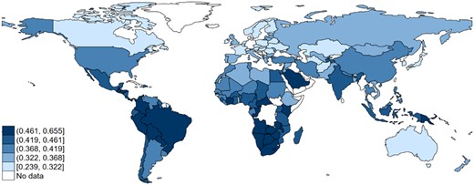
Cross-country differences in Gini.
2.3 Deep-rooted genetic distance
Spolaore and Wacziarg (2009) use the genetic distance index to capture long-term relatedness between countries. This indicator, developed based on the original genetic data of Cavalli-Sforza et al. (1994), reflects the difference in the distributions of genes between populations. More specifically, genetic distance is captured by the index of ‘expected heterozygosity’, which corresponds to the probability of genetic dissimilarity between two individuals randomly selected from a relevant population with respect to a given cluster of genetic markers (Ashraf and Galor, 2018). The ‘expected heterozygosity’ index is constructed by population geneticists based on data on allele frequencies, such as the frequency of occurrence of a gene variant (or allele) within a given population (Ashraf and Galor, 2018). Hence, two populations characterized by greater differences in the allele distributions are more genetically distant to each other. By contrast, genetically closer populations are those bearing greater similarities in the allele distributions.
Only neutral genes, of which the changes are random and independent of selection pressure, are considered when constructing the genetic distance index (Spolaore and Wacziarg, 2009). As most random changes in the distributions of genes occur regularly over time, genetic distance corresponds to the length of time elapsed since two populations were separated from a common ancestor driven by random genetic mutations over time (Cavalli-Sforza et al., 1994). This yields a comparable proxy for long-term relatedness between countries measured by the divergence in the distributions of neutral genes. To the extent that many human traits and characteristics are transmitted across generations with variation, genetically distant populations characterized by longer periods of ancestral separation tend to diverge in a variety of inter-generationally transmitted traits, such as norms, values, beliefs, predispositions, languages, and preferences. I use Nei’s (1972) measure of genetic distance to capture cross-country differences in genetic distance to Denmark (Gdist_DNK) as depicted in Figure 2.
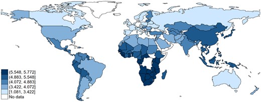
Cross-country differences in Gdist_DNK.
2.4 Main control variables
To mitigate plausible concerns about omitted variable bias, I incorporate several control variables in the baseline model. More specifically, a key challenge with estimating Equation (1) is that the long-term distributional legacy of Gdist_DNK can be attributed to various country-level fundamental factors that drive worldwide comparative development, such as geographic characteristics. For instance, Michalopoulos (2012) finds that Terrain Ruggedness is linked to the emergence of diverse social groups across geographically fragmented areas within a country. In addition, Elevation and the suitability of land areas for agricultural activities (Landsuit) have a persistent influence on population diversity, thus shaping long-run development (Michalopoulos, 2012). These geographic covariates, by increasing population diversity, could affect heterogeneity in preferences for redistributive policies and measures, thereby driving income inequality (Arbatlı et al., 2020; Vu, 2021a).
Moreover, the existing literature has established that Absolute Latitude, distance to the nearest waterway (Distcoast), Landlockedness, and the proportion of lands in tropics and subtropics (Landtrstr) help shape long-run comparative development through institutional, climatological, and trade-related mechanisms (see Arbatlı et al., 2020). In this regard, these geographic attributes plausibly matter for egalitarian income (re)distribution. Furthermore, geographical factors could affect genetic relatedness between societies via driving genetic drift and mutations throughout human history. The baseline model specification is augmented with the set of main geographic controls, including Absolute Latitude, Distcoast, Landlockedness, Terrain Ruggedness, Landsuit, Elevation, and Landtrstr. To control for unobserved region-specific (time-invariant) factors, I include dummy variables for East Asia and Pacific, Europe and Central Asia, Latin America and Caribbean, Middle East and North Africa, North America, and South Asia in the regression (sub-Saharan Africa is excluded as the base category).
3. Main results
Figure 3 presents a cross-plot for Gdist_DNK and Gini. It reveals that countries with greater genetic distance to Denmark have higher levels of disposable income inequality, consistent with the main hypothesis.
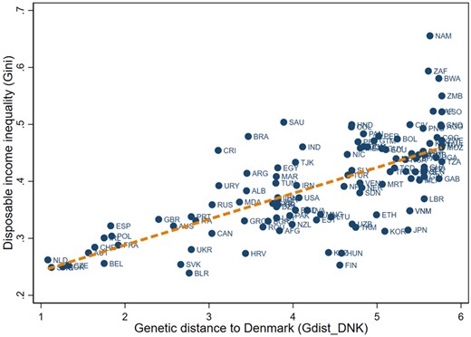
Scatter plot for Gdist_DNK and Gini.
3.1 OLS estimates
Table 2 contains OLS estimates of the effect of Gdist_DNK on disposable income inequality (Columns 1 and 2). I include the set of main geographic/agroclimatic controls in column (1). The benchmark model is also augmented with region dummies as shown in column (2). Accordingly, Gdist_DNK enters all the regressions with a positive and statistically significant coefficient. This lends support to the hypothesized relationship between Gdist_DNK and Gini. Furthermore, the magnitude and statistical significance of the estimated coefficient on Gdist_DNK remain insensitive to controlling for geographic characteristics and unobserved time-invariant heterogeneity across world regions. According to the baseline estimates, an extra standard deviation of Gdist_DNK is associated with an approximately 0.028-unit increase in Gini, holding other things equal (Column 2, Table 2). This equates to a third of a standard deviation of Gini, which is suggestive of the economic significance of the estimated impact of genetic distance on disposable income inequality. Overall, the OLS results indicate that genetic distance to Denmark has a statistically and economically significant impact on disposable income inequality across countries.1 Hence, genetic distance is a major barrier to achieving egalitarian income distribution within a country. This is attributed to the role of genetic distance in shaping the cross-border diffusion of redistributive policies and measures. Specifically, countries with longer periods of ancestral separation from the global frontier of income distribution are more likely to suffer from barriers to adopting effective fiscal redistribution, leading to greater income disparities.
The effect of Gdist_DNK on disposable income inequality, main results
| Dep_var: Gini | OLS estimates | IV estimates | ||
|---|---|---|---|---|
| (1) | (2) | (3) | (4) | |
| Gdist_DNK | 0.021*** | 0.022*** | 0.026*** | 0.019*** |
| [0.006] | [0.005] | [0.007] | [0.006] | |
| Absolute latitude | −0.199*** | −0.081 | −0.175*** | −0.086 |
| [0.053] | [0.065] | [0.052] | [0.060] | |
| Distcoast | −0.001 | −0.001 | −0.001 | −0.001 |
| [0.002] | [0.002] | [0.002] | [0.001] | |
| Landlockedness | −0.021 | −0.021 | −0.019 | −0.019 |
| [0.015] | [0.015] | [0.015] | [0.015] | |
| Terrain ruggedness | −0.012* | −0.004 | −0.011* | −0.004 |
| [0.007] | [0.005] | [0.006] | [0.005] | |
| Landsuit | −0.002 | −0.015 | −0.004 | −0.012 |
| [0.023] | [0.023] | [0.023] | [0.021] | |
| Elevation | 0.006*** | 0.005*** | 0.006*** | 0.005*** |
| [0.002] | [0.001] | [0.002] | [0.001] | |
| Landtrstr | −0.003 | 0.004 | −0.005 | 0.006 |
| [0.021] | [0.021] | [0.021] | [0.020] | |
| IV (First-stage) estimates. Dep_var: Gdist_DNK | ||||
| Gdist_1500 | 0.402*** | 0.414*** | ||
| [0.045] | [0.045] | |||
| Region dummies | No | Yes | No | Yes |
| Observations (number of countries) | 118 | 118 | 116 | 116 |
| R-squared | 0.635 | 0.709 | 0.624 | 0.702 |
| F-statistic of the joint significance of control variables [p-value] | 6.59 | 9.77 | 37.47 | 144.11 |
| [0.000] | [0.000] | [0.000] | [0.000] | |
| First-stage F-statistic | 80.15 | 84.01 | ||
| Anderson–Rubin confidence intervals | [0.013, 0.039] | [0.007, 0.030] | ||
Notes: This table reports empirical estimates of the effect of Gdist_DNK on Gini. Robust standard errors in squared brackets.
p < 0.01,
p < 0.05,
p < 0.1.
Source: Author’s calculations.
A key concern about the plausibility of the main results relates to potential measurement errors in the main outcome variable. It is argued that Gini might not be constructed in a consistent manner across countries, making it difficult to obtain an internationally comparable measure of inequality. This issue stems from the prevalence of informal income, low tax compliance, and a lack of adequate social welfare policies in many developing economies. To address this concern, I replicate the main analysis by using alternative measures of socio-economic inequality, as depicted in Figure 4. It is noteworthy that different proxies for inequality typically vary in terms of country coverage and the welfare definition employed (e.g., consumption or income). Hence, I use four alternative measures of inequality proxied by the shares of income and wealth owned by the top 1% and 10% of the population, provided by the World Inequality Database (WID) (https://wid.world). These alternative outcome variables are constructed using various data sources, including household surveys, tax data, inheritance records, and national accounts, thereby offering internationally comparable measures of inequality across countries and over time (Blanchet et al., 2020).2 I also use a measure of net income inequality provided by the World Income Inequality Database (WIID). Additionally, I exploit the welfare inequality indicator developed by the World Bank’s Poverty and Inequality Platform (https://pip.worldbank.org/home). This index, in particular, reflects inequality of income or consumption in different countries depending on whether the income or consumption approach is more relevant for measuring welfare. As depicted in Figure 4, the coefficient on Gdist_DNK remains positive in all cases, in line with my prediction. The estimated effect of Gdist_DNK on inequality is also statistically significant at conventionally accepted levels, except when using the top 1% wealth share from the WID as the outcome variable. Overall, these results consistently reveal that Gdist_DNK is a major barrier to establishing an egalitarian society.

The effects of Gdist_DNK on alternative measures of economic inequality.
3.2 Instrumental variable estimates
A key challenge with identification relates to potential endogeneity bias induced by unobserved confounding characteristics and/or measurement errors in Gdist_DNK. In particular, there exist many country-specific factors that cannot be identified and incorporated in the regression. To the extent that Gdist_DNK is correlated with unobserved confounders that are relevant for explaining worldwide differences in income distribution, the main results can be biased and inconsistent. For example, achieving a causal interpretation of the main results critically requires some attention to factors shaping the worldwide variation in genetic distance. As argued by Spolaore and Wacziarg (2016c), the driving forces of genetic relatedness typically differ between the Old World (Eurasia and Africa) and the New World (the Americas and Oceania). More specifically, differences in the allele distributions between populations in the Old World were largely determined by exogenous geographical and biogeographical factors in prehistoric times (before 1500CE). This is because long-term relatedness in the Old World was predominantly shaped over the prehistoric course of the exodus of Homo sapiens from East Africa starting around tens of thousands of years ago before the process of modern nation-state building (Cavalli-Sforza et al., 1994; Bellwood, 2014). For this reason, the distribution of genetic distance in the Old World is plausibly unrelated to forces shaping contemporary economic development, thus offering exogenous variation in today’s income inequality. Nevertheless, plausible endogeneity concerns mainly stem from mass post-1500 migration flows to the New World, leading to persistent variation in current-day genetic distance and economic development. One could argue that the divergence in contemporary income distribution can be attributed to the aforementioned geographic characteristics that shaped the pattern of European colonization around 1500CE, causing persistent differences in contemporary institutions and policies.
In line with Spolaore and Wacziarg (2009), I address the above concern by using genetic distance to the English population in 1500CE (Gdist_1500) to generate a plausibly exogenous source of variation in Gdist_DNK. To the extent that Gdist_1500 was predetermined by the prehistoric course in which H. sapiens gradually populated the entire globe, it is unlikely to be affected by contemporary income distribution. Moreover, predetermined Gdist_1500 affects Gini exclusively via shaping today’s genetic relatedness (via genetic drift or mutations over time) because it is presumably unrelated to factors driving contemporary income distribution. This lends support to the validity of the exogeneity condition. Spolaore and Wacziarg (2009) also highlight that the construction of Gdist_1500 is less likely to suffer from measurement errors because the original data on genetic distance were collected by Cavalli-Sforza et al. (1994) for ancestral populations in 1500CE. Hence, the process of matching the data of populations to countries would be easier for 1500 than for the post-1500 period as the former does not require tracing the ancestral origins of current-day New World populations. The instrumental variable (IV) estimates indicate that Gdist_DNK has a positive and statistically significant impact on Gini (Columns 2 and 3, Table 2). It follows from the first-stage estimates that Gdist_1500 is strongly correlated with Gdist_DNK, suggesting that the IV is relevant. Following the recommendation of Andrews et al. (2019), I report the first-stage F-statistic of excluded instruments developed by Olea and Pflueger (2013). As shown in Table 2, the F-statistic is much larger than the rule-of-thumb value of 10, thus mitigating concerns about weak instrument bias. Additionally, Andrews et al. (2019) suggest reporting identification-robust Anderson–Rubin confidence intervals regardless of the first-stage F-values. Hence, I construct and report these in Table 2, and all exclude zero. This is suggestive of the statistically significant influence of Gdist_DNK on Gini irrespective of the relevance of the IV in the first-stage regression. Overall, I consistently find precise estimates of the positive impact of the plausibly exogenous component of Gdist_DNK on Gini.
3.3 Long-term persistence
This article establishes that long-term relatedness between populations provides a fundamental explanation for worldwide differences in income inequality. As explained earlier, genetic distance impedes the international diffusion of redistributive policies and measures, thus triggering initial variation in inequality across countries. Given that genetic distance is a proxy for the duration of ancestral separation between populations, the global divergence in income inequality attributed to genetic distance would exhibit a remarkable degree of persistence over time. This is consistent with the idea of ‘long-term persistence’ in comparative economic development (Guiso et al., 2016). The main findings reveal that long-term relatedness between countries is highly predictive of cross-country differences in Gini averaged between 2000 and 2015. However, the level of inequality has witnessed an increasing trend over the last decades. This justifies the motivation of examining evidence of persistence in the role of Gdist_DNK in shaping international differences in egalitarian income distribution.
For this purpose, I follow Maseland (2021) to regress Gini for each year between 1990 and 2015 on Gdist_DNK. I also augment all these repeated cross-sectional regressions with the set of main control variables. A key challenge with this empirical exercise is that the comparability of the empirical estimates derived from these regressions can be confounded by changes in the feasible sample size stemming from measuring the dependent variables in different years. Hence, I use Gini for each year of the period 1900–2015 as the dependent variables to obtain comparable samples of countries. Additionally, I estimate the repeated cross-sectional regressions using the top 10% income share taken from the WID for each year between 1980 and 2021 as alternative outcome variables. Figure 5 illustrates the point estimate and 95% confidence interval of the coefficient on Gdist_DNK. Consistent with my prediction, the coefficient on Gdist_DNK remains positive and precisely estimated at conventionally accepted levels of statistical significance in all cases. These results suggest that long-term relatedness between countries consistently plays a key role in driving cross-country differences in egalitarian income distribution over years. A possible explanation is that the worldwide distribution of income inequality fundamentally driven by long-term relatedness exhibits a remarkable degree of persistence over time albeit an increasing trend in inequality in several countries. Therefore, the results depicted in Figure 5 provide evidence of the persistent impact of Gdist_DNK on disposable income inequality between 1980 and 2021.
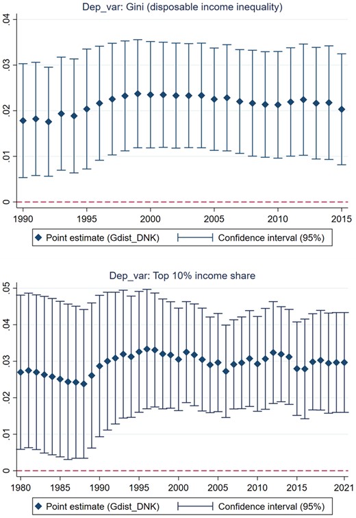
‘Long-term persistence’ in the distributional impact of Gdist_DNK.
Notes: This figure illustrates the effect of Gdist_DNK on two alternative measures of inequality from estimating numerous repeated cross-sectional regressions. All the regressions are augmented with key control variables.
4. Robustness checks and extensions
4.1 Controlling for the ‘proximate’ causes of inequality
To rule out the possibility that the main results can be confounded by conventional explanations of worldwide differences in income inequality, I allow additional control variables to enter the model specifications; the results are reported in Table 3. Specifically, I control for log of GDP per capita (Lgddpc) and its quadratic term (Lgddpc_sqr) following Kuznets (1955). Motivated by Gupta et al. (2002), I augment the regression analysis with the average of six dimensions of governance (Institutions). I also follow Sturm and De Haan (2015) to control for two alternative proxies for population diversity, including Fractionalization (Alesina et al., 2003) and Polarization (Desmet et al., 2012).3 Consistent with a review of the existing literature by Furceri and Ostry (2019), I incorporate trade openness (Trade), financial development (Credit), age dependency ratio (Age), and the quality of human capital (Hci) in the regressions. In all cases, the core results withstand their signs and statistical precision. Thus, the distributional legacy of long-term relatedness between countries is unlikely to be confounded by the ‘proximate’ determinants of income inequality.
Controlling for the ‘proximate’ causes of income inequality
| (1) | (2) | (3) | (4) | (5) | (6) | (7) | (8) | |
|---|---|---|---|---|---|---|---|---|
| Panel A. OLS estimates. Dep_var: Gini | ||||||||
| Gdist_DNK | 0.020*** | 0.027*** | 0.023*** | 0.022*** | 0.020*** | 0.022*** | 0.020*** | 0.024*** |
| [0.005] | [0.007] | [0.006] | [0.005] | [0.005] | [0.005] | [0.006] | [0.007] | |
| Panel B. IV (Second-stage) estimates. Dep_var: Gini | ||||||||
| Gdist_DNK | 0.018*** | 0.023*** | 0.020*** | 0.019*** | 0.016** | 0.017*** | 0.015** | 0.015** |
| [0.006] | [0.008] | [0.006] | [0.006] | [0.006] | [0.006] | [0.006] | [0.007] | |
| Panel C. IV (First-stage) estimates. Dep_var: Gdist_DNK | ||||||||
| Gdist_1500 | 0.406*** | 0.389*** | 0.410*** | 0.412*** | 0.397*** | 0.415*** | 0.386*** | 0.362*** |
| [0.042] | [0.050] | [0.047] | [0.046] | [0.040] | [0.045] | [0.048] | [0.051] | |
| Lgdppc | Yes | Yes | ||||||
| Lgdppc_sqr | Yes | Yes | ||||||
| Institutions | Yes | Yes | ||||||
| Fractionalization | Yes | Yes | ||||||
| Polarization | Yes | Yes | ||||||
| Trade | Yes | Yes | ||||||
| Credit | Yes | Yes | ||||||
| Age | Yes | Yes | ||||||
| Hci | Yes | Yes | ||||||
| Geographic/agroclimatic controls | Yes | Yes | Yes | Yes | Yes | Yes | Yes | Yes |
| Region dummies | Yes | Yes | Yes | Yes | Yes | Yes | Yes | Yes |
| Observations | 114 | 117 | 117 | 118 | 112 | 118 | 109 | 101 |
| First-stage F-statistic | 91.97 | 59.48 | 76.37 | 79.63 | 99.64 | 85.19 | 64.27 | 50.57 |
| [Anderson–Rubin confidence intervals] | [0.006, 0.030] | [0.008, 0.038] | [0.008, 0.032] | [0.007, 0.030] | [0.004, 0.028] | [0.0005, 0.028] | [0.003, 0.027] | [0.002, 0.028] |
Notes: This table replicates the main analysis by controlling for the conventional ‘proximate’ determinants of income inequality.
Source: Author’s calculations.
4.2 Controlling for the fundamental causes of inequality
The main results can also be confounded by slowly evolving characteristics that fundamentally drive cross-country differences in income inequality. Previous studies, for example, emphasize the importance of colonial legacies in shaping long-run development (La Porta et al., 1999; Acemoglu et al., 2001; Easterly and Levine, 2016). Accordingly, inherited colonial rule and the identity of the former colonial powers have a persistent impact on today’s institutions and economic performance, and hence affect contemporary income distribution (Vu, 2021a). For this reason, I incorporate binary variables for colonial rule (Colonial dummies) and inherited legal traditions (LO dummies) in the regression. Motivated by Naveed and Wang (2018), I control for the proportion of the population practicing major religions (Religion). Consistent with Vu (2021a), I allow the state history index developed by Borcan et al. (2018) to enter the regression in a quadratic form.
Other scholars suggest that deep-rooted genetic diversity undermines the ability to establish egalitarian income (re)distribution by giving rise to heterogeneity in interpersonal preferences for the provision of public goods (Ashraf and Galor, 2018; Arbatlı et al., 2020; Vu, 2021b). It is also argued that highly diverse countries tend to suffer from persistent mistrust, thus hampering long-run development (Ashraf and Galor, 2013; Arbatlı et al., 2020; Vu, 2021c).4 Therefore, I include the ancestry-adjusted genetic diversity index (Pdiv_aa) constructed by Ashraf and Galor (2013) in the regression.5 Following Arbatlı et al. (2020), I control for accumulated experience with democratic and autocratic political regimes between 1960 and 2017 (Democratic and Autocratic experience). Nikolaev et al. (2017) place emphasis on the distributional impact of the cultural dimension of individualism/collectivism. Therefore, I include individualism and social trust in the baseline model. Controlling for these additional factors, however, does not affect the relationship between Gdist_DNK and Gini (Table 4).
Controlling for the fundamental causes of income inequality
| (1) | (2) | (3) | (4) | (5) | (6) | (7) | (8) | (9) | |
|---|---|---|---|---|---|---|---|---|---|
| Panel A. OLS estimates. Dep_var: Gini | |||||||||
| Gdist_DNK | 0.022*** | 0.020*** | 0.022*** | 0.021*** | 0.023*** | 0.026*** | 0.023*** | 0.017*** | 0.020*** |
| [0.006] | [0.005] | [0.006] | [0.005] | [0.005] | [0.006] | [0.006] | [0.006] | [0.006] | |
| Panel B. IV (Second-stage) estimates. Dep_var: Gini | |||||||||
| Gdist_DNK | 0.017*** | 0.018*** | 0.019*** | 0.012** | 0.019*** | 0.021*** | 0.020*** | 0.014** | 0.012** |
| [0.006] | [0.006] | [0.006] | [0.006] | [0.006] | [0.007] | [0.007] | [0.006] | [0.006] | |
| Panel C. IV (First-stage) estimates. Dep_var: Gdist_DNK | |||||||||
| Gdist_1500 | 0.415*** | 0.405*** | 0.406*** | 0.428*** | 0.412*** | 0.408*** | 0.363*** | 0.417*** | 0.383*** |
| [0.046] | [0.046] | [0.057] | [0.046] | [0.046] | [0.047] | [0.058] | [0.064] | [0.076] | |
| Colonial dummies | Yes | Yes | |||||||
| LO dummies | Yes | Yes | |||||||
| Religion | Yes | Yes | |||||||
| Statehiste | Yes | Yes | |||||||
| Statehiste_sqr | Yes | Yes | |||||||
| Pdiv_aa | Yes | Yes | |||||||
| Democratic experience | Yes | Yes | |||||||
| Autocratic experience | Yes | Yes | |||||||
| Individualism | Yes | Yes | |||||||
| Social trust | Yes | Yes | |||||||
| Geographic/agroclimatic controls | Yes | Yes | Yes | Yes | Yes | Yes | Yes | Yes | Yes |
| Region dummies | Yes | Yes | Yes | Yes | Yes | Yes | Yes | Yes | Yes |
| Observations | 118 | 118 | 118 | 118 | 118 | 118 | 83 | 75 | 66 |
| First-stage F-statistic | 82.93 | 76.48 | 50.83 | 87.04 | 81.04 | 74.99 | 39.73 | 42.23 | 25.14 |
| [Anderson–Rubin confidence intervals] | [0.004, 0.029] | [0.007, 0.029] | [0.007, 0.031] | [0.0004, 0.023] | [0.008, 0.031] | [0.008, 0.033] | [0.008, 0.033] | [0.001, 0.026] | [−0.001, 0.023] |
Notes: This table replicates the main analysis by controlling for the fundamental drivers of income inequality.
Source: Author’s calculations.
4.3 Fixed effects filtered estimates
A major issue with estimating the benchmark model is that the results can be explained away by unobserved country-specific factors. However, the parameter of interest would not be identified if I were to include country-fixed effects (FE) in the regression because the FE transformation eliminates all time-invariant covariates. As reviewed by Furceri and Ostry (2019), the evolution of income inequality within countries over time can be driven by several time-varying socio-economic characteristics. The presence of such confounding factors, if not being explicitly accounted for, may yield an invalid basis for statistical inference on the relationship between Gdist_DNK and Gini.
To address this concern, I employ the FEs filtered estimator developed by Pesaran and Zhou (2018). This method is suitable for examining the effect of a time-invariant variable in panel data models where N is large, and T is small and fixed. The implementation of this method follows a two-step regression procedure. In the first step, I estimate panel data models for 104 countries spanning the period 1990–2015. In particular, I regress the Gini coefficient of disposable income inequality on its time-varying determinants, including the linear and quadratic terms of log of GDP per capita, age dependence ratio, financial development, trade openness, human capital, and the quality of governance following Furceri and Ostry (2019). The regression is augmented with country and year FEs to account for unobserved country- and year-specific factors. Then, I calculate the predicted residuals and average them between 1990 and 2015. In the second-step regression, I re-estimate the baseline cross-sectional model using the time averages of the residuals as an alternative outcome variable. As shown in Online Appendix Table A1, the coefficient on Gdist_DNK remains positive and precisely estimated at conventionally accepted levels of statistical significance. This suggests that the core findings are insensitive to accounting for unobserved country- and year-specific factors, and several time-varying observed confounders.
4.4 Other sensitivity tests
To check whether the main results are attributed to the inclusion of specific groups of countries with similar histories, cultures, and geography, I replicate the main analysis using different sub-samples of countries. I also exclude potential outliers from the regression and re-estimate the benchmark model. Furthermore, I calculate Conley’s standard errors that correct for potential spatial autocorrelation in the error terms. My findings remain intact in all cases (see Online Appendix Tables A2–A4). As discussed earlier, my findings are robust to controlling for the potential deep determinants of inequality, but this does not necessarily imply that long-term relatedness between countries is the only fundamental driver of income distribution across the world. If two countries have similar levels of genetic distance to the selected base country but differ in income inequality, other countries’ fundamental characteristics could be relevant for explaining such outliers. Motivated by Vu (2021a), I test for the interactional effect between state history and Gdist_DNK on Gini. The results, available on request, show that the interaction term is negative and statistically significant at the 5% level, which suggests that accumulated statehood experience helps mitigate the detrimental impact of genetic distance on income distribution.6 In this regard, a potential avenue for future research is to explore the role of other countries’ fundamental characteristics in shaping the distributional legacy of genetic distance, which is important for policy interventions.
4.5 Further evidence from a bilateral approach
I now move towards exploring the extent to which genetic distance between countries affects bilateral differences in income inequality. Specifically, a bilateral approach permits examining whether country pairs with greater genetic distance are characterized by larger absolute differences in income inequality due to barriers to the cross-border diffusion of redistributive policies and measures, and institutions. Hence, I specify the following model.
where
Genetic distance and bilateral differences in income inequality
| Dep_var: Absolute difference in Gini | OLS estimates | IV estimates | ||||
|---|---|---|---|---|---|---|
| (1) | (2) | (3) | (4) | (5) | (6) | |
| Gdist | 0.504*** | 0.663*** | 0.518*** | 1.762*** | 2.235*** | 1.628** |
| [0.068] | [0.079] | [0.085] | [0.334] | [0.520] | [0.762] | |
| Geographic distance | 0.216*** | 0.193*** | 0.217*** | 0.104*** | 0.048 | 0.119 |
| [0.017] | [0.019] | [0.027] | [0.035] | [0.052] | [0.074] | |
| Contiguity | 0.350 | 0.665* | 0.467 | 0.884** | 1.227** | 0.819 |
| [0.289] | [0.364] | [0.393] | [0.362] | [0.479] | [0.501] | |
| Absolute difference in Absolute Latitude | 0.183*** | 0.121*** | 0.121*** | 0.168*** | 0.112*** | 0.113*** |
| [0.006] | [0.007] | [0.007] | [0.007] | [0.007] | [0.009] | |
| Absolute difference in Distcoast | −0.001*** | −0.001*** | −0.001*** | −0.001*** | −0.001*** | −0.001*** |
| [0.000] | [0.000] | [0.000] | [0.000] | [0.000] | [0.000] | |
| A dummy for difference in Landlockedness | 0.963*** | 1.311*** | 1.265*** | 0.924*** | 1.339*** | 1.270*** |
| [0.144] | [0.160] | [0.168] | [0.146] | [0.163] | [0.168] | |
| Absolute difference in Terrain Ruggedness | −0.004*** | −0.005*** | −0.006*** | −0.004*** | −0.005*** | −0.006*** |
| [0.001] | [0.001] | [0.001] | [0.001] | [0.001] | [0.001] | |
| Absolute difference in Landsuit | 1.751*** | 1.862*** | 2.577*** | 1.916*** | 1.972*** | 2.600*** |
| [0.330] | [0.360] | [0.393] | [0.334] | [0.365] | [0.393] | |
| Absolute difference in Elevation | 0.0004*** | 0.001*** | 0.001*** | 0.0004** | 0.001*** | 0.001*** |
| [0.0002] | [0.0002] | [0.0002] | [0.0002] | [0.0002] | [0.0002] | |
| Absolute difference in Landtrstr | −0.073 | 0.227 | 0.078 | −0.599** | −0.331 | −0.213 |
| [0.210] | [0.223] | [0.234] | [0.238] | [0.284] | [0.296] | |
| IV (First-stage) estimates. Dep_var: Gdist | ||||||
| Gdist_1500 | 2.109*** | 1.549*** | 1.125*** | |||
| [0.098] | [0.119] | [0.123] | ||||
| Absolute difference in the proximate causes of Gini | No | Yes | Yes | No | Yes | Yes |
| Absolute difference in the fundamental causes of Gini | No | No | Yes | No | No | Yes |
| Pairwise region dummies | Yes | Yes | Yes | Yes | Yes | Yes |
| Observations (number of country pairs) | 9,423 | 7,358 | 6,763 | 9,423 | 7,358 | 6,763 |
| R-squared | 0.273 | 0.342 | 0.350 | 0.165 | 0.230 | 0.262 |
| First-stage F-statistic | 459.99 | 168.49 | 82.89 | |||
| [Anderson–Rubin confidence intervals] | [1.133, 2.391] | [1.258, 3.213] | [0.194, 3.213] | |||
Notes: This table reports empirical estimates of the effect of genetic distance on bilateral differences in income inequality.
Source: Author’s calculations.
5. Mechanisms
5.1 Gdist_DNK and preferences for equality among second-generation Europeans
The reduced-form relationship between Gdist_DNK and Gini is primarily explained by the role of long-term relatedness between countries in driving the worldwide dissemination of redistributive policies and measures. A possible explanation is that genetically proximate countries tend to have similar preferences over the provision of public goods, or, more broadly, income redistribution, thereby enhancing policy emulation and adoption. This line of reasoning rests upon the argument that genetic distance between populations is conducive to the divergence in numerous inter-generationally transmitted traits, including values, beliefs, predispositions, and preferences, thus shaping cross-border interactions, communications, and knowledge exchanges. To provide empirical support for these propositions, I use individual-level data from nine rounds of the European Social Survey between 2002 and 2020. Specifically, I exploit variation in Gdist_DNK of the country of origin of second-generation Europeans (e.g., EU-born individuals whose parents are foreign-born) to explain differences in surveyed respondents’ attitudes towards equality. This allows examining whether genetic distance helps shape heterogeneity in interpersonal preferences towards redistribution. I propose that Europeans descending from countries with greater Gdist_DNK are less likely to exhibit positive attitudes towards equality.
To capture individuals’ preferences for equality, I rely on survey participants’ responses to the statement that ‘it is important that people are treated equally and have equal opportunities’. I create a dummy variable taking a value of one if survey participants’ responses are recorded as ‘very much like me’, ‘like me’, or ‘somewhat like me’. By contrast, the dummy variable is assigned a value of zero if the answers are recorded as ‘a little like me’, ‘not like me’, or ‘not like me at all’. The empirical analysis is carried out using three different samples of second-generation immigrants to European countries. I first consider EU-born individuals whose parents are from the same foreign country to account for the confounding impact of the mixture of different cultures. I also adopt alternative samples of Europeans whose father and/or mother are from a foreign country. It is noteworthy that using data for second-generation Europeans helps control for many unobserved confounding characteristics, which would be the case when using those for first-generation immigrants (e.g., socio-economic discrimination or language/cultural barriers).
I include country-of-residence FEs in the regression to explore whether Gdist_DNK helps explain the variation in attitudes towards equality among second-generation immigrants residing in the same European country who are presumably exposed to similar institutions and many other country-level socio-economic characteristics. In line with the main analysis, I augment the individual-level regressions with several geographic/agroclimatic characteristics of the country of origin. I account for round-specific factors by incorporating survey round FEs in the regression. Furthermore, a number of individual characteristics are allowed to enter the regression model. I cluster the standard errors at the country-of-origin level. The results indicate that Gdist_DNK of the country of origin is negatively associated with preferences for equality among second-generation Europeans (Table 6). The coefficient on Gdist_DNK remains statistically significant at the 1% or 5% levels in all cases. This provides support for the central hypothesis that genetic distance, by increasing the divergence in individual-level preferences for redistribution between countries, hampers the international diffusion of redistributive policies and measures, and hence leads to a more unequal distribution of income.
The effect of Gdist_DNK on preferences for equality, individual-level evidence
| Second-generation Europeans | (1) | (2) | (3) |
|---|---|---|---|
| Parents are from the same foreign country | Father is from a foreign country | Mother is from a foreign country | |
| Dep_var: Preferences for equality | |||
| Gdist_DNK | −0.049*** | −0.051*** | −0.027** |
| [0.019] | [0.016] | [0.013] | |
| Country-of-origin controls | Yes | Yes | Yes |
| Individual-level controls | Yes | Yes | Yes |
| Country-of-residence FE | Yes | Yes | Yes |
| Survey round FE | Yes | Yes | Yes |
| Observations | 20,728 | 30,661 | 29,778 |
| Pseudo R-squared | 0.033 | 0.038 | 0.038 |
Notes: This table reports probit estimates of the effect of Gdist_DNK of the country of origin on preferences for equality among second-generation Europeans (e.g., EU-born individuals whose parents are foreign-born). Country-of-origin controls include Absolute Latitude, Distcoast, Landlockedness, Terrain Ruggedness, Landsuit, Elevation, and Landtrstr. Individual-level controls include a dummy variable for female, the linear and quadratic term of age, employment status, and dummy variables for educational attainment and income status. Robust standard errors, clustered at the country-of-origin level, in squared brackets.
p < 0.01,
p < 0.05,
p < 0.1.
Source: Author’s calculations.
5.2 The average controlled direct effect of Gdist_DNK on Gini
The main findings suggest that countries with longer periods of ancestral separation from Denmark find it more difficult to establish an equal distribution of income. In this regard, a better understanding of the underlying mechanisms is important for formulating relevant policies that help attenuate such disadvantages. To check for the proposed mechanisms, I capture international differences in effective fiscal redistribution by the absolute (aRedist) and relative (rRedist) differences between market and disposable income inequality using data from the SWIID, following Berg et al. (2018) and Solt (2020).7 Consistent with Vu (2022), I also use public expenditure on health (Healthexp) and education (Eduexp) as a proportion of total GDP to measure the government’s efforts to redistribute income. Additionally, I calculate the average of six dimensions of worldwide governance to measure institutional quality (Institutions). Then, I investigate the role of aRedist, rRedist, Healthexp, and Eduexp (mediators) in driving the relationship between Gdist_DNK and Gini across countries.
Prior to exploring the underlying mechanisms, I regress potential mediating covariates on Gdist_DNK and the set of key control variables. Consistent with my prediction, I find that Gdist_DNK has a negative and statistically significant impact on aRedist and rRedist (Online Appendix Table A5). Furthermore, countries that are genetically distant to Denmark tend to exhibit less redistributive effort proxied by public expenditure on health. However, the impact of Gdist_DNK on Eduexp is imprecisely estimated at conventional levels of statistical significance. The results also reveal that Gdist_DNK exerts a negative influence on the quality of institutions. Therefore, Gdist_DNK helps explain cross-country differences in redistribution and institutional quality, which are key to shaping income inequality.
Following Acharya et al.’s (2016) adoption of sequential g-estimation, I implement their two-stage estimation method to examine whether the aforementioned mechanisms play a key role in explaining the main findings. The first-stage regression involves regressing Gini on Gdist_DNK, the mediator(s) (e.g., aRedist), and the set of control variables including pre-treatment variables and intermediate confounders. Next, I calculate the transformed (demediated) outcome variable by removing the impact of the mediator. In the second-stage regression, I regress the demediated outcome variable on Gdist_DNK and the pre-treatment controls, excluding all the intermediate confounders from the regression. This yields the average controlled direct effect (ACDE) of Gdist_DNK on Gini, holding the potential mediator(s) fixed at a particular level. I treat the baseline geographic/agroclimatic controls and region dummies as pre-treatment covariates as they are alternative fundamental causes of income inequality. Intermediate confounders are variables that are shaped by Gdist_DNK and have an impact on Gini. Hence, I treat the ‘proximate’ determinants of income inequality included in Table 3 as the intermediate confounders.
Figure 6 depicts the ACDE results. Compared with the core results, the ACDE estimates turn out to be less precise when controlling for the impact of aRedist. There exist substantial reductions in the magnitude and statistical precision of the coefficient on Gdist_DNK when I account for the mediating impact of rRedist. However, the ACDE estimates display trivial changes, relative to the total effect, when I partial out the distributional impacts of Healthexp, Eduexp, and Institutions. Therefore, I find evidence that effective fiscal redistribution is a key mechanism underlying the main findings of this article.
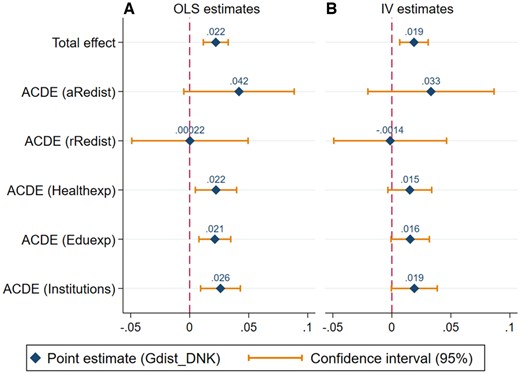
The ACDE of Gdist_DNK on Gini.
Notes: This figure illustrates the ACDE results. For instance, ACDE (rRedist) reflects the distributional effect of Gdist_DNK when holding rRedist fixed at a particular level. For ease of interpretation, I also replicate the baseline estimates (total effect). See Online Appendix Table A6 for the full estimates.
6. Concluding remarks
This article examines the role of long-term relatedness between countries in shaping worldwide differences in disposable income inequality. It proposes and empirically establishes the hypothesis that genetic distance to the world frontier of income distribution impedes the cross-border diffusion of redistributive policies and measures and institutions, leading to greater income inequality. Using cross-country data, I find that countries with greater genetic distance to Denmark have higher levels of disposable income inequality, ceteris paribus. The main results withstand numerous robustness exercises. Based on bilateral data, I document that genetic distance is positively associated with the absolute differences in income inequality between countries. The individual-level analysis reveals that genetic distance to Denmark increases the divergence in preferences for equality between countries. Furthermore, effective fiscal redistribution is a key mechanism through which genetic distance to Denmark transmits to higher income inequality. Therefore, effective policy interventions towards less inequality at least partially require strong commitments to establishing progressive income redistribution. This helps mitigate the persistent impact of long-term relatedness between countries on income inequality.
Supplementary material
Supplementary material is available on the OUP website. It contains data, replication code, and an Online Appendix.
Funding
The author received no financial support for this work.
Footnotes
The main results are robust to using Finland, Sweden, and Norway as the frontier country (Online Appendix Figure A1). According to Kleven (2014), these Scandinavian countries are characterized by very low tax evasion, high tax-to-GDP ratio, and generous welfare policies that help reduce income inequality. In addition, the core findings do not hold when using Slovenia as the base country although it is among the most egalitarian countries worldwide (Online Appendix Figure A1). As suggested by an anonymous reviewer, Slovenia’s low levels of income inequality are primarily attributed to redistribution through taxes and transfers adopted within a transitional economy.
Using an extended sample of 139 countries, based on data from the WID, helps rule out the possibility that the main results can be confounded by failure to include several (developing) countries where data on Gini are not available.
Becker (1957) puts forward that people tend to exhibit greater empathy preferentially towards members of their own group. Thus, ethnically fragmented countries are less likely to implement redistribution, which is key to reducing inequality (Desmet et al., 2012). For example, many American countries are endowed with much higher levels of ethnic fractionalization and income inequality, compared with their European counterparts. To the extent that ethnolinguistic fractionalization is linked to societal non-cohesiveness and heterogeneity in preferences for public goods provision, it plausibly undermines egalitarian income (re)distribution (Alesina et al., 2003; Desmet et al., 2012; Arbatlı et al., 2020). Therefore, existing differences in income inequality between several European and American countries can be attributed to their divergence in ethnolinguistic fractionalization.
According to the ‘out of Africa’ theory of comparative development of Ashraf and Galor (2013), the prehistoric course of the exodus of H. sapiens from East Africa has a persistent influence on cross-country differences in genetic diversity, thereby driving worldwide comparative development. Specifically, African societies, which are among the most genetically fragmented countries, tend to suffer from persistent underdevelopment due to the detrimental effect of diversity on social trust and public goods provision. Incorporating the genetic diversity index and dummy variables for African countries in the regression helps address a key concern that the main results can be confounded or driven by the inclusion of highly heterogeneous African countries.
This empirical exercise allows checking whether Gdist_DNK matters for cross-country differences in income inequality holding within-population genetic diversity fixed at a particular level. A potential avenue for future research is to explore whether genetic diversity within countries affects egalitarian income distribution through shaping mutual trust and heterogeneity in interpersonal preferences for public goods provision.
East Asian economies, relative to their European counterparts, have comparable levels of income inequality but higher degrees of Gdist_DNK. It has been established that East Asian economies, such as Japan, South Korea, and Taiwan, maintained robust economic growth over a long period, driven by land reform policies and structural transformation towards producing high-productivity products (Studwell, 2013). Such policies attributed to strong state capacity are arguably important for reducing poverty and inequality in East Asia (Vu, 2021a). By contrast, Latin American countries, characterized by significantly weaker statehood experience, tend to suffer from a more unequal distribution of land and income (see Guereña, 2016).
Specifically,
Acknowledgements
My gratitude goes to Professor Dorian Owen for many helpful discussions during early stages of this research. I also thank two anonymous reviewers for several useful suggestions that improved the article. The usual disclaimer applies.
