


ABSTRACT
Although the MEST-C classification is among the best prognostic tools in immunoglobulin A nephropathy (IgAN), it has a wide interobserver variability between specialized pathologists and others. Therefore we trained and evaluated a tool using a neural network to automate the MEST-C grading.
Biopsies of patients with IgAN were divided into three independent groups: the Training cohort (n = 42) to train the network, the Test cohort (n = 66) to compare its pixel segmentation to that made by pathologists and the Application cohort (n = 88) to compare the MEST-C scores computed by the network or by pathologists.
In the Test cohort, >73% of pixels were correctly identified by the network as M, E, S or C. In the Application cohort, the neural network area under the receiver operating characteristics curves were 0.88, 0.91, 0.88, 0.94, 0.96, 0.96 and 0.92 to predict M1, E1, S1, T1, T2, C1 and C2, respectively. The kappa coefficients between pathologists and the network assessments were substantial for E, S, T and C scores (kappa scores of 0.68, 0.79, 0.73 and 0.70, respectively) and moderate for M score (kappa score of 0.52). Network S and T scores were associated with the occurrence of the composite survival endpoint (death, dialysis, transplantation or doubling of serum creatinine) [hazard ratios 9.67 (P = .006) and 7.67 (P < .001), respectively].
This work highlights the possibility of automated recognition and quantification of each element of the MEST-C classification using deep learning methods.
What is already known about this subject?
The MEST-C classification is an international consensus-based classification linked to kidney prognosis in immunoglobulin A nephropathy (IgAN).
The MEST-C grading lacks reproducibility between specialized pathologists and others.
To obtain a reliable and reproducible evaluation of this classification, we trained and evaluated a tool using a neural network.
What this study adds?
In this study, we developed an image analysis of IgAN kidney biopsies stained with Masson's trichrome.
This tool using deep learning can automatically perform the MEST-C classification.
This automated evaluation provided results close to those of four trained kidney pathologists.
What impact this may have on practice or policy?
This new deep learning methodology for scoring the MEST-C could change our approach to IgAN.
We hope that this tool will help to pinpoint lesions and reduce interobserver variability.
A better assessment of MEST-C classification could improve patients management.
INTRODUCTION
Immunoglobulin A nephropathy (IgAN) is the most common primary glomerulonephritis worldwide [1]. This disease is caused by glomerular deposits of degalactosylated IgA1, which can locally lead to inflammation, fibrosis and nephron destruction [2]. There is a great disparity in the evolutionary profiles of patients with IgAN. Some will only suffer from chronic benign haematuria, while others will rapidly progress to end-stage kidney disease [2, 3]. Apart from supportive care, the aetiological treatment is not strictly codified [4, 5]. Nonetheless, some studies have highlighted a beneficial impact of corticosteroid treatment in patients at risk of progression [4, 6, 7]. Rauen et al. [4] showed an impact on the proteinuria whereas Lv et al. [6] showed an impact on the eGFR decline. Therefore, a better assessment of kidney prognosis seems mandatory to adapt monitoring and therapeutic management.
The MEST-C score is an international consensus-based classification of IgAN that identifies and quantifies kidney histological lesions [8, 9]. It was designed by the Working Group of the International IgA Nephropathy Network and the Renal Pathology Society [8]. This classification is currently one of the best prognostic tools in IgAN patients [3, 10–20]. Yet, the multiplicity of features and the low reproducibility limit its use [11, 19, 21, 22] particularly for endocapillary lesions as discussed by Roberts [21]. In the study of Bellur et al. [23], the mesangial hypercellularity, endocapillary hypercellularity and crescent had poor interrater reproducibility between an expert and a non-expert pathologist. The use of the MEST-C score is thus limited in non-specialized pathology centres.
Convolutional neural networks (CNNs) have recently led to many advances in kidney pathology. Our team and others have demonstrated the feasibility of automated segmentation of kidney histological structures from digitized biopsy images [24–27]. We have thus trained a CNN on two datasets that enable us to obtain a precise and reproducible measurement of interstitial fibrosis and tubular atrophy (IF/TA) [24]. Extending this work to get an automated MEST-C score could improve reproducibility. This preliminary study sought to set up and evaluate a deep learning–based methodology to automatically evaluate each element of the MEST-C classification.
MATERIALS AND METHODS
Patients
Included patients underwent a kidney biopsy at the French University Hospital of Dijon between January 2010 and January 2020 or of Besançon between January 2016 and January 2020. Only biopsies associated with a diagnosis of IgAN were included. IgA vasculitis biopsies were excluded in MEST-C grading and prognosis evaluation (Application cohort). Transplanted kidneys, glomerulonephritis secondary to infection and lupus were excluded. Patients had to be ≥14 years of age.
Clinical and biological data at the time of the biopsy were retrospectively collected for all patients, including age, sex, serum creatinine (SCr), proteinuria, renin–angiotensin system inhibitors and immunosuppressive regimen. The evaluation of the estimated glomerular filtration rate (eGFR) was performed using the Chronic Kidney Disease Epidemiology Collaboration formula. Follow-up data up to January 2022 were collected for patients included in the Application cohort. When available, proteinuria (n = 57) and eGFR (n = 70) at 1 year of follow-up were collected and their variations from baseline values were calculated. The survival composite endpoint was the occurrence of death, transplantation, dialysis or the doubling of SCr. The end of follow-up was the date of either the last visit, death, transplantation or dialysis. Patients gave oral informed consent before the study. This work complied with the Helsinki Declaration and was approved by the local ethics committee.
Kidney biopsies
Kidney biopsies were formalin fixed, paraffin embedded and cut into 2-μm sections. To match with our previous CNN algorithm, only Masson's trichrome stains were evaluated (125 green, 71 blue) [24]. Nanozoomer 2.0 C9600-12 (Hamamatsu Photonics, Hamamatsu, Japan) was used to digitize biopsy slides. The initial image resolution was 454 nm/pixel. Samples of cortical images designated as regions of interest (ROI) were annotated (Analytical Solutions and Products, Amsterdam, The Netherlands) at a magnification of 200×. Whole slide images were inferred at a magnification of 25×.
Training, Test and Application cohorts
A total of 196 IgAN kidney biopsies were split into three independent cohorts. Forty-two were randomly selected to be included in the Training cohort. Among the remaining biopsies, primary IgAN with less than eight non-globally sclerotic glomeruli (NGSG) or IgA vasculitis were included in the Test cohort and primary IgAN greater than eight NGSG were included in the Application cohort. For the Training and Test cohorts, annotations of the histological lesions were blindly made. The annotated ROI was used to train the CNN in the Training cohort and was compared with automated predictions for the Test cohort (n = 66). The evaluation of the Application cohort (n = 88) was performed on whole biopsies of primary IgAN. It compared automated predictions by CNN to the gold standard visual scores. This gold standard was obtained by merging independent evaluations made by four kidney pathologists with a French degree in kidney pathology (two individual analyses and one made by two pathologists together). The gold standard results were the mean of pathologists’ lesions scores. In case of disagreement for endocapillary hypercellularity, active crescent or sclerosis lesions, the four pathologists reviewed the biopsy to reach a consensus decision.
Neural network
Training and evaluations were carried out on a PC Titan RTX (Nvidia, Santa Clara, CA, USA) graphics card (24 GB VRAM). The CNN used was a Mask R-CNN Inception ResNet V2 from the Tensorflow/models GitHub repository. The only data modification performed was a spatial augmentation, with a 50% probability at each epoch (number of times the algorithm worked through the entire training).
None of the biopsies from the Test and Application cohorts were used for CNN trainings. The first algorithm aimed at detecting the cortical and medullary areas and the capsule. The second one, limited to the previously delineated cortical area, aimed to detect NGSG, globally sclerotic glomeruli, arteries, veins and healthy and atrophic tubules. The last algorithm evaluated within the previously selected NGSG the areas of mesangial hypercellularity (M), endocapillary hypercellularity (E), active crescent (C), segmental sclerosis (S), vascular stalk and necrosis.
The first and second algorithms were based on those previously carried out (see Supplementary Methods) [24]. To improve the performance of the second algorithm for the segmentation of NGSG with lesions, ROIs were added to this training. A total of 2798 vignettes from 227 regions were trained on 135 epochs [24]. The third algorithm used ROIs centred on the NGSG. During the sequence of the CNN, pre-processing was set up to create vignettes (1024 × 1024 pixels) centred on the NGSG previously detected. A total of 467 vignettes from 425 regions were used for this training on 400 epochs. Respectively, 473 M, 782 E, 217 S, 131 C, 94 necrosis and 130 vascular stalks were annotated (Supplementary Table 1). Inferred images were post-processed to merge masks from different vignettes and filter masks according to pre-established rules. The same 152 ROIs were used to assess the Test cohort of the second and third algorithms. The tool is freely available online (https://github.com/SkinetTeam/Skinet-MEST-C; Supplementary Methods).
Histological analysis of the Application cohort
Within the Application cohort, manual and automated analyses counted the glomeruli and the M, E, S, C and necrosis objects. Hypercellularity lesions inside the vascular stalk were excluded [8]. The percentage of NGSG with lesions was obtained. The percentage of IF/TA was assessed with a step of 5 for visual analysis. In the CNN analysis, the percentage of IF was assessed by the cortical area not annotated by the second algorithm relative to the total cortical area. TA was assessed by the number of atrophic tubules relative to the number of total tubules [24]. We assessed the mean bias of the algorithm's assessment for each criterion using Bland–Altman analyses. The evaluation of MEST-C was based on the previous definitions [9, 11]. An automated iMEST-C was based on the predictions of the CNN after we applied a corrective factor (derived from the mean bias previously observed). This calibrating factor was applied to the percentages of glomeruli with M and/or C, the number of glomeruli with E, S and/or C and the percentage of IF/TA to predict iM1, iC2, iE1, iS1, iC1 and iT1-2, respectively. This iMEST-C calibrated in the Application cohort was used to evaluate the interrater reliability and the kidney prognosis.
Junior pathologists
Three resident trainees in kidney pathology were considered as junior pathologists. They blindly graded the biopsies from the Application cohort. After a week of washout, they evaluated the biopsies knowing the CNN's predictions (marked with false colours, as shown in Fig. 1).
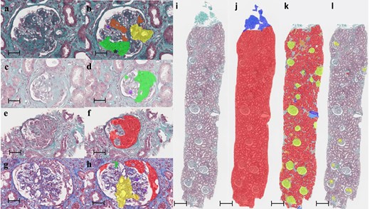
Evaluation by the algorithms of kidney lesions in IgAN. Kidney biopsies stained with Masson's trichrome. Comparison of images before processing (a, e, c, g) and after processing (b, f, d, h) by the third algorithm focused on glomerular lesions. Scale bars: 50 µm, 400× magnification. The lesions on the treated images were automatically and artificially coloured in red, green, purple, orange and yellow for lesions of the crescent, glomerular sclerosis, endocapillary hypercellularity, mesangial hypercellularity and vascular stalk, respectively. *Abnormally segmented endocapillary hypercellularity within fibrosis area. (i–l) Kidney biopsy M0E1S1T0C0 of a patient evaluated by the three consecutive neural network algorithms. Scale bars: 500 µm, 25× magnification. (i) Biopsy before segmentation. (j) Biopsy after segmentation by the first algorithm to isolate the cortical area. The capsule is coloured in blue and the cortex in red. (k) Cortical area isolated after segmentation by the second algorithm to assess T status and isolate glomeruli. Glomeruli are coloured in yellow, healthy tubules in red, atrophic tubules in orange, arteries in dark blue and veins in light blue. (l) Glomeruli within the cortical zone after segmentation by the third neural network to calculate M, E, S and C scores. There is an area falsely identified as a crescent.
Statistical analysis
Quantitative data were expressed as mean ± standard deviation (SD) or median [interquartile range (IQR)] depending on whether the distribution was normal or not. Comparisons of two variables were made with the Student’s t-test or Mann–Whitney test depending on whether the distribution was normal or not. For the comparison of more than two variables, a Kruskal–Wallis test was used. Correlations were calculated using a Spearman test. Semi-quantitative variables were expressed as number (percentage).
Performance for the detection and classification of objects was assessed by calculating Precision (percentage of items belonging to a class among all the items predicted to belong to it), Recall (percentage of items predicted to belong to a class among all the items belonging to it) and F-score: [2 × (Precision × Recall)/(Precision + Recall)] (Supplementary Fig. 1). Intersection Over Union (IOU) was also calculated: (common area between the predicted and the annotated object)/(area of the predicted object + area of the annotated object − common area) (Supplementary Fig. 2) [28]. Kappa coefficients were used as measures of interrater reliability. A kappa score <0.40 is poor, 0.40–0.59 is moderate, 0.60–0.79 is substantial and 0.80 is outstanding [29]. ROC curves were used to evaluate the prediction power of our algorithm (our classifier) for each MEST-C criterion. Bland–Altman analyses were conducted for bias evaluation.
Univariate survival analyses were performed with a logrank test. The statistical analyses were performed using GraphPad Prism 6.01 (GraphPad Software, San Diego, CA, USA) and SPSS 23 (IBM, Armonk, NY, USA).
RESULTS
Population characteristics
Among the 196 included patients who provided a biopsy sample, the mean age at inclusion was 48 ± 19 years and 73% (n = 143) were men. At the time of biopsy, mean SCr, eGFR and proteinuria were 2.2 ± 2.1 mg/dL, 61±41 ml/min/1.73 m2 and 2.7 ± 2.6 g/day, respectively. The distribution of biopsies in each cohort and the clinical and biological data of the patients are described in Fig. 2 and Table 1.
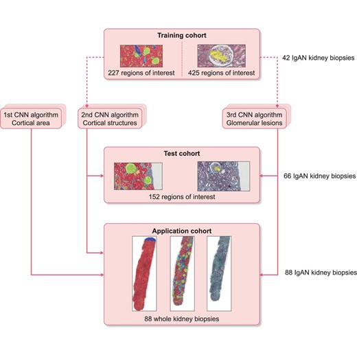
Distribution of kidney biopsies among the Training, Test and Application cohorts. The dotted arrows represent the use of CNN for training and the continuous arrows represent the use of CNN for inference. None of patients from the Application and Test cohorts were used for trainings.
Population characteristics.
| Data | Total populationa (N = 196) | Training cohorta (n = 42) | Test cohorta (n = 66) | Application cohort (n = 88) |
|---|---|---|---|---|
| Age (years), mean ± SD | 48 ± 19 | 47 ± 19 | 49 ± 20 | 47 ± 19 |
| Male, n (%) | 143 (73) | 28 (67) | 47 (71) | 68 (77) |
| Primary IgAN, n (%) | 159 (81%) | 32 (76) | 39 (59) | 88 (100) |
| IgA vasculitis, n (%) | 37 (19) | 10 (24) | 27 (41) | 0 (0) |
| Diabetes mellitus, n (%) | 26 (13) | 4 (10) | 11 (17) | 11 (13) |
| Hypertension at biopsy, n (%) | 124/195 (63) | 22/41 (54) | 46/65 (70) | 56 (63) |
| Renin–angiotensin system inhibitors (within 3 months after biopsy), n (%) | 133/192 (69) | 28/38 (74) | 50 (76) | 55 (63) |
| Immunosuppressant (within 3 months after biopsy), n (%) | 67/191 (35) | 14/40 (35) | 25/64 (39) | 28/87 (30) |
| eGFR at biopsy (ml/min/1.73 m2), mean ± SD | 61 ± 41 | 71 ± 42 | 51 ± 39 | 63 ± 40 |
| SCr at biopsy (mg/dl), mean ± SD | 2.2 ± 2.1 | 1.8 ± 1.6 | 2.4 ± 2.1 | 2.1 ± 2.4 |
| Haematuria at biopsy, n (%) | 172/183 (94) | 36/40 (90) | 59/62 (95) | 77/81 (95) |
| Gross haematuria, n (%) | 31/183 (17) | 6/40 (15) | 13/62 (21) | 12/81 (15) |
| Urine protein level at biopsy (g/day), mean ± SD | 2.7 ± 2.6 | 2.8 ± 2.5 | 2.6 ± 2.2 | 2.8 ±2.9 |
| Non-globally sclerotic glomeruli (number), mean ± SD | 13 ± 8 | 16 ± 9 | 8 ± 7 | 16 ±7 |
| Globally sclerotic glomeruli (number), mean ± SD | 3 ± 4 | 3 ± 4 | 3 ± 4 | 3 ±4 |
| Percentage of non-globally sclerotic glomeruli (%),mean ± SD | 80 ± 23 | 82 ± 23 | 73 ± 28 | 86 ± 15 |
| M1, n (%) | 21 (24) | |||
| E1, n (%) | 39 (45) | |||
| S1, n (%) | 63 (72) | |||
| T1, n (%) | 35 (40) | |||
| T2, n (%) | 9 (10) | |||
| C1, n (%) | 18 (20) | |||
| C2, n (%) | 12 (14) |
aNo evaluation of the MEST-C classification was performed due to an insufficient number of non-globally sclerotic glomeruli in some biopsies.
Comparisons of segmentations in the Test cohort
In the Test cohort, the second algorithm had a good capacity to identify the pixels of tubules and glomeruli (>87% of the corresponding pixels were correctly segmented). The weakest discriminative abilities were those of atrophic tubules and veins (87% and 70% of pixels correctly segmented, respectively) (Supplementary Fig. 3, Supplementary Table 2). The pixel confusion matrix for this algorithm is shown in Fig. 3. More than 80% of the pixels of the M, S and C lesions were correctly identified. The E class had the lowest recognition rate (73% of pixels correctly identified). The F-scores and IOU showed good lesion recognition performance (Table 2). The most common predictions errors are described in Supplementary Fig. 4.
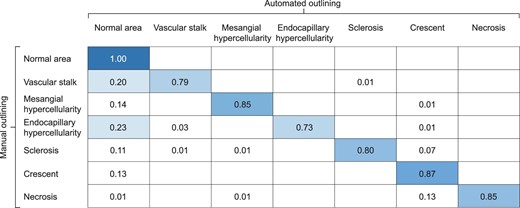
CNN confusion matrix per pixel assessing glomerular lesions within regions of interest in the Test cohort. For example, for pixels having been manually assigned to the mesangial hypercellularity category, the neural network correctly predicted the category for 85% of those pixels.
Ability of classification of the glomerular CNN in the Test cohort.
| Objects | Precisiona | Recallb | F-scorec | IOUd |
|---|---|---|---|---|
| Vascular stalk | 0.90 | 0.89 | 0.89 | 0.64 |
| Mesangial hypercellularity | 0.85 | 0.83 | 0.84 | 0.77 |
| Endocapillary hypercellularity | 0.83 | 0.75 | 0.79 | 0.65 |
| Segmental sclerosis/adhesion | 0.88 | 0.67 | 0.76 | 0.75 |
| Active crescent | 0.79 | 0.66 | 0.72 | 0.67 |
| Necrosis | 0.68 | 0.96 | 0.80 | 0.73 |
aPrecision (positive predictive value): percentage of items belonging to the class of interest among items identified as belonging to the class of interest.
bRecall (sensitivity): percentage of items identified as belonging to the class of interest among all items belonging to the class of interest.
cF-score: 2 × (Precision × Recall)/(Precision + Recall).
dIOU: (common area between the predicted and the annotated object)/(area of the predicted object + area of the annotated object − common area of the annotated and predicted object).
MEST-C in the Application cohort
This cohort aimed to compare pathologists’ and CNN assessments on whole biopsies of primary IgAN (Supplementary Fig. 5). The mean inference time per biopsy was 39 ± 21 min. There was a strong association between the predicted and observed percentages of M, C and IF/TA (r = 0.71, 0.75 and 0.85, respectively; all P < .001) and between the number of NGSG with observed and predicted E, S and C (r = 0.75, 0.61 and 0.77, respectively; all P < .001). The Bland–Altman analyses for bias calculation and calibration are described in Fig. 4 and Supplementary Fig. 6. The ROC curves of the three algorithms to predict M1, E1, S1, T1, T2, C1, C2 and fibrinoid necrosis had areas under the curve (AUCs) of 0.88 [95% confidence interval (CI) 0.81–0.95], 0.91 (95% CI 0.86–0.98), 0.88 (95% CI 0.79–0.97), 0.94 (95% CI 0.89–0.98), 0.96 (95% CI 0.92–0.99), 0.96 (95% CI 0.93–0.99), 0.92 (95% CI 0.85–0.99) and 0.81 (95% CI 0.71–0.91), respectively, with all P < .001 (Supplementary Fig. 7). The kappa coefficients between pathologists and the CNN assessments were substantial for E0–1, S0–1, T0–1/2 and C0–1/2 (with kappa scores of 0.68, 0.79, 0.73 and 0.70, respectively) but were moderate for M0–1 (kappa score of 0.52). The gold standard evaluations compared with the pathologists’ and CNN assessments are presented in Fig. 5. The interrater agreement scores between pathologists are described in Supplementary Table 3.
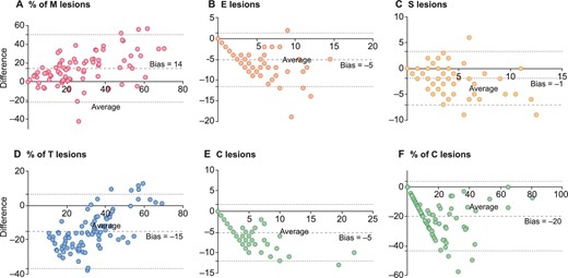
Bland–Altman plot between lesions observed and predicted in the Application cohort. The mean bias is represented by the large dashed black lines with the 95% limits of agreement represented by the small dashed lines.
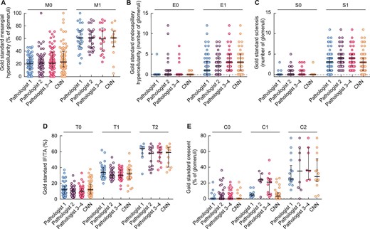
Gold standard evaluations compared with the pathologists’ scores. The bars correspond to the medians and the scales to the IQR.
Junior pathologists’ evaluations
The mean kappa coefficients of the three junior pathologists were poor to moderate and inferior to the CNN's predictions for M0–1, E0–1, S0–1, T0–1/2 and C0–1/2 (mean kappa scores of 0.45, 0.21, 0.35, 0.56 and 0.26, respectively) (Supplementary Fig. 8). After a second evaluation with the CNN's help, the kappa coefficients were slightly increased for M0–1, S0–1 and T0–1/2 (mean kappa scores of 0.47, 0.38 and 0.61, respectively) and decreased for E0–1, C0–1/2 (mean kappa scores of 0.19, and 0.21, respectively) (Supplementary Table 3).
Follow-up
In the Application cohort, mean SCr, eGFR and proteinuria at biopsy were 2.1 ± 2.4 mg/dl, 63 ± 40 ml/min/1.73 m2 and 2.8 ± 2.9 g/day. Patients with iS1, iT1–2, iC1–2 had significantly lower eGFR at biopsy compared with patients free of these lesions (Supplementary Fig. 9). At 1 year, the mean percentages of eGFR and proteinuria variations from baseline values were 29 ± 85% and −26 ± 79%, respectively. While the percentage of iS was associated with the eGFR Delta (r = −0.29, P = .034), the percentage of iM lesions was associated with the proteinuria Delta (r = −0.33, P = .011). Of note, correlation between iC/iT lesions and proteinuria Delta did not reach significance (P = .089 and P = .083, respectively).
During a mean follow-up of 41 ± 36 months, 4 (5%) patients died, 13 (15%) patients had to start dialysis, none had a transplantation and 23 (26%) had at least one of the individual outcomes of the survival composite endpoint (death, transplantation, dialysis or doubling of SCr). In univariate analysis, iS1, iT1, S1 and T1 status were associated with the occurrence of the survival composite endpoint [hazard ratio 9.67 (95% CI 1.44–10.31), P = .006; 7.67 (95% CI 2.91–14.95), P < .001; 5.41 (95% CI 1.32–7.24), P = .010 and 14.80 (95% CI 3.53–17.80), P < .001, respectively]. Only the T score was associated with the composite endpoint among the junior pathologists (Table 3). At follow-up, the mean percentage eGFR variation from baseline was 9 ± 97%. iS and iT were associated with the mean percentages of eGFR variation (r = −0.33, P = .003 and r = −0.31, P = .004, respectively) but the trend with iC did not reach significance (r = −0.21, P = .062).
Survival analysis of the composite criteria death, transplantation, dialysis or doubling of SCr in the Application cohort.
| Factors | Hazard ratio (95% confidence interval) | P-value |
|---|---|---|
| Age (per year) | 1.05 (1.02–1.08) | .002 |
| Male | 1.47 (0.57–3.80) | .421 |
| Hypertension | 1.71 (0.51–5.81) | .381 |
| Diabetes mellitus | 1.17 (0.39–3.47) | .780 |
| Renin–angiotensin system inhibitors | 0.95 (0.41–2.24) | .909 |
| Immunosuppressive therapy | 1.95 (0.86–4.43) | .105 |
| SCr at biopsy (per 0.1 mg/dl) | 1.18 (1.07–1.29) | <.001 |
| Proteinuria at biopsy (per 0.1 g/day) | 1.13 (1.02–1.27) | .023 |
| M1 gold standard | 2.31 (1.01–6.63) | .034 |
| E1 gold standard | 1.19 (0.54–2.68) | .655 |
| S1 gold standard | 5.41 (1.32–7.24) | .010 |
| T (1/2 versus 0) gold standard | 14.80 (3.53–17.80) | <.001 |
| C (1/2 versus 0) gold standard | 0.95 (0.42–2.10) | .889 |
| iM1 | 1.29 (0.49–3.53) | .591 |
| iE1 | 1.53 (0.69–3.58) | .317 |
| iS1 | 9.67 (1.44–10.31) | .006 |
| iT (1/2 versus 0) | 7.67 (2.91–14.95) | <.001 |
| iC (1/2 versus 0) | 1.26 (0.55–2.86) | .589 |
| M1 junior pathologist 1 | 1.73 (0.73–4.64) | .198 |
| E1 junior pathologist 1 | 1.66 (0.55–4.34) | .409 |
| S1 junior pathologist 1 | 1.54 (0.61–3.69) | .383 |
| T1/2 versus 0) junior pathologist 1 | 4.84 (1.46–7.90) | .005 |
| C (1/2 versus 0) junior pathologist 1 | 1.34 (0.51–3.27) | .598 |
| M1 junior pathologist 2 | 1.31 (0.34–4.97) | .701 |
| E1 junior pathologist 2 | 1.20 (0.46–3.09) | .719 |
| S1 junior pathologist 2 | 1.99 (0.38–7.47) | .491 |
| T1/2 versus 0) junior pathologist 2 | 3.96 (1.03–6.60) | .044 |
| C (1/2 versus 0) junior pathologist 2 | 2.35 (0.85–4.97) | .110 |
| M1 junior pathologist 3 | 1.84 (0.76–5.39) | .163 |
| E1 junior pathologist 3 | 1.07 (0.42–2.69) | .894 |
| S1 junior pathologist 3 | 1.04 (0.25–4.35) | .959 |
| T1/2 versus 0) junior pathologist 3 | 1.40 (1.06–5.76) | .039 |
| C (1/2 versus 0) junior pathologist 3 | 1.01 (0.41–2.48) | .986 |
Survival analyses were performed with a logrank test.
P-values of the factors statistically associated with the endpoint occurence are bolded.
DISCUSSION
This work highlights the possibility of automated recognition and quantification of each element of the MEST-C classification using deep learning methods. The CNN had a good ability to predict the concerted scores of four pathologists.
About 30% of the patients with IgAN will progress to end-stage kidney disease [2]. While other studies have used CNN on extracted data from IgAN patients’ records to develop prediction models for prognosis, we used CNN to automate a histological classification [30–32]. Indeed, recent work from Bellur et al. [23] observed poor reproducibility between local and central pathologists for M, E and C of the MEST-C. The advantage of segmentation by CNN is its reproducibility and accuracy and we think that better reproducibility would increase the scores utility and help patient management [22]. Another work has recently shown the potential for deep learning analysis of IgAN kidney biopsies. In that work, the training was performed without manual segmentation of the lesions [33]. Therefore the lesions could not be individually identified by the network, and apart from fibrosis, the results of the neural network correlated very little with the MEST-C criteria. We chose to automate the recognition of the lesions that are known for having an impact on renal prognosis [10, 12, 13, 20, 34]. To the best of our knowledge, this is the first CNN-based tool to provide a fully automated assessment of an entire international consensus-based classification with interstitial, tubular and glomerular lesions.
Zeng et al. [35] previously developed a tool for glomerular lesion recognition in IgAN biopsies. Their evaluation of segmental sclerosis and crescents yielded a kappa >0.78, while the mesangial score had a kappa of 0.42. In our study, >80% of M, S and C pixels were correctly segmented. We observed kappa close to that of Zeng et al. for S and C scores (0.79 and 0.70, respectively). We also faced the same limitation of moderate interrater reliability with the M score (kappa of 0.52), mainly related to incomplete recognition of areas with mesangial hypercellularity by the CNN. The performances of the CNNs (in both studies) might be enhanced by adding more images with mesangial hypercellularity in the training process. Perhaps a combination of machine learning and deep learning techniques would be better suited for this type of recognition. It should be noted that in the study of Zeng et al. [35], the training of intraglomerular mesangial hypercellularity was only performed in 240 ROI of NGSG with neither sclerosis nor crescents (versus 425 ROI with various lesions in our study). In addition, it did not allow recognition of endocapillary hypercellularity or IF/TA. Our algorithm also had a good capacity to predict the E, S and C scores with AUCs >80%. Given that MEST-C scoring can lead to significant clinical decisions, further studies are necessary to reach a better reliability. E lesions are known to suffer from low interrater reliability [9, 23]. In our study, even if the CNN tended to confuse endothelial cells with endocapillary proliferative ones, the interrater reliability was substantial and higher than expected. As the number of E lesions per affected glomerulus tended to be high, a relatively high number of E objects were included in the training, which could partly explain this good reliability. As the CNN tended to have a bias with systematic over- or underestimation of lesions, we added the bias values from the Bland–Altman analyses to calibrate the tool. This seemed necessary because the tool tends to overestimate E, S and C lesions and the presence of a single lesion is enough to score E1, S1 and C1. More training with more glomerular lesions could have improved these results.
The T score is a semi-quantitative evaluation of IF/TA. We used precise segmentation of the cortical elements to assess it. This evaluation of IF/TA is close to that of Hermsen et al. [25]. The number of objects used in the second training was not less than in previous publications [24, 25, 27]. We also added new ROIs to our previously published tool to enhance recognition of NGSG with hypercellularity or sclerosis [24]. The performance was equivalent to those previously published and even higher than our previous study (notably for atrophic tubules) [24, 25, 27]. Contrary to many studies, we used a specific algorithm to delineate the cortical area away from other structures [24], so that no manual segmentation was needed before assessing the IF/TA. We observed a good ability to detect T1 and T2 scores (AUC of 0.94 and 0.96, respectively).
Patients with iS1, iT1–2 and iC1–2 scores had a lower initial eGFR than those without. These observations are consistent with those of local pathologists and those previously published [23]. Unlike pathologists’ evaluations, CNN-assessed M and E scores were not associated with an initial worsening in eGFR. While the percentage of iS, iT and iC lesions tended to be correlated with eGFR variation at follow-up, the percentage of iM lesions on initial kidney biopsy was correlated with the proteinuria decrease at 1 year. In univariate analysis, iT1–2 and iS1 scores were associated with a higher risk of premature death, transplantation, dialysis or doubling of SCr. Unlike our local evaluation, no effect was observed with the M score on kidney survival. This was probably linked to the moderate reliability between iM and M scores. Even if the lack of association between proliferative scores and kidney survival weakens our results, several larger published IgAN studies have similar results [3, 16, 17, 19]. E, C and sometimes M scores are inconsistently associated with the patient's prognosis. However, the association between iMEST-C score, renal prognosis and response to immunosuppressive therapies needs to be evaluated in a larger independent cohort before this can be applied in clinical practice. No multivariate analysis and no subgroup analysis in patients with different treatment regimens were performed, as the number of events and treated patients was insufficient. The immunosuppressive treatments might have masked the impact of the E or C score [7, 12, 20]. A relatively short follow-up and small population could also explain why these scores did not reach significance. In addition, only one biopsy section per patient was used. However, the MEST-C is based on the evaluation of several sections and stains [8, 9].
To assess the potential impact of this CNN in regions lacking kidney pathologists, the biopsies were also analysed by trainees. The interrater agreement between them and the gold standard was lower than between the CNN and our gold standard, but was close to that between an expert and a non-expert [9, 16, 23]. Unlike the CNN, the S1 scores of each junior pathologist were unrelated to the composite endpoint. One could imagine using these CNNs in the absence of available specialists. Nevertheless, the use of CNN visual markers to help junior pathologists has shown only a moderate and inconsistent contribution.
Periodic acid–Schiff stain is classically recommended to evaluate the MEST-C score [23]. Indeed, cellularity is better assessed in tissue sections stained with periodic acid–Schiff [21]. Thus the use of Masson's trichrome limits the generalization of this study. We used Masson's trichrome, as our previously published algorithm to evaluate T scores and to isolate glomeruli was only trained and evaluated on this stain [24]. Masson's trichrome tends to highlight more sclerotic lesions, which could explain the high proportion of patients scored as S1 [36]. The eGFR at biopsy and the prognoses of the patients were more severe than in most studies [16, 19]. We believe that this is partly due to a restrictive kidney biopsy policy in our centres. This could also partly explain the increased observed number of E lesions [16, 23]. Even if larger studies had similar E1 scores, a centre effect with overestimation of the E parameter cannot be ruled out [12, 17, 34]. It is also the authors’ belief that Masson's trichrome tends to overestimate endocapillary hypercellularity due to poorer delineation of endothelial surfaces. As the CNN has never encountered other stains during training, it cannot be used with other stains. Thus another study with periodic acid–Schiff stain training is mandatory.
The MEST-C was initially developed to assess the prognosis of primary IgAN. However, many studies have shown that kidney biopsy of IgA vasculitis could be graded using the MEST-C [37–39]. Some patients with IgA vasculitis were included in the Training and Test cohorts to increase the number of ROI. Nevertheless, the MEST-C was not designed to evaluate the prognosis of those patients [40, 41] and Davin pointed out that the extra-renalmanifestations of IgA vasculitis are not the only difference with IgAN [40]. Thus only primary IgAN patients were evaluated in the Application cohort for MEST-C grading and prognosis purposes.
This new deep learning methodology for scoring the MEST-C could change our approach towards IgAN. Nevertheless, an larger external validation study is needed to assess its potential prognostic capacity and generalization.
ACKNOWLEDGEMENTS
An abstract from part of this work was presented at the 2022 ERA/EDTA Congress.
FUNDING
This work was funded by the NEPHRIN-APJ2019 (Appel d'offre jeunes chercheurs) GIRCI EST (47 755 euros) (to M.L.).
AUTHORS’ CONTRIBUTIONS
A.J., E.M. and M.L. contributed equally to this work as first and last authors. A.J., E.M., G.T., M.P., L.M., J.M.R. and M.L. were responsible for conception and analysis and interpretation of data. A.J., E.M. and M.L. drafted the article. M.C., M.F.V., M.C., C.R., D.D., T.C., S.F., A.J. and D.C. helped with data acquisition and analysis. G.T., L.M., M.F.V. and M.L. evaluated the kidney biopsies. E.M., M.C. and C.R. were the junior pathologists. C.T. and G.Z. provided intellectual content of critical importance to the work described. All authors approved the final version to be published.
DATA AVAILABILITY STATEMENT
The three algorithms are freely available at https://github.com/SkinetTeam/Skinet-MEST-C and the tutorials to use them and infer your images are located in the ‘docs’ folder. The data underlying this article will be shared upon reasonable request to the corresponding author.
CONFLICT OF INTEREST STATEMENT
None declared.


Comments