


Abstract
A fundamental analysis task for single-cell transcriptomics data is clustering with subsequent visualization of cell clusters. The genes responsible for the clustering are only inferred in a subsequent step. Clustering cells and genes together would be the remit of biclustering algorithms, which are often bogged down by the size of single-cell data. Here we present ‘Correspondence Analysis based Biclustering on Networks’ (CAbiNet) for joint clustering and visualization of single-cell RNA-sequencing data. CAbiNet performs efficient co-clustering of cells and their respective marker genes and jointly visualizes the biclusters in a non-linear embedding for easy and interactive visual exploration of the data.
Introduction
Visualization and clustering of cells are key tasks in the analysis of single-cell transcriptomics data. The genes common to the cells in a cluster and thus contributing as possible marker genes to the definition of a cell type are determined in subsequent differential expression analysis. The expectation is that given an overall similarity among cells in a cluster, these cells will share the relevant marker genes without a clustering program paying particular attention to this goal. Here, we want to remedy this problem by, from the beginning of the analysis, clustering and visualizing cells and genes jointly. Such a joint visualization of cells and genes together with their grouping into joint clusters aids in determination of marker genes, in interpretation of clusters and in assessment of clustering quality.
Principal component analysis (PCA) or the lesser known correspondence analysis (CA) represents given data in a high-dimensional space (1). A projection into, e.g. a plane may then help the visualization, but for complex data sacrifices too much information. Instead, it has become a common practice in single-cell RNA sequencing (scRNA-seq) to apply non-linear embedding methods like t-SNE (2) or UMAP (3) for visualization purposes. Using CA as a starting point rather than PCA has the advantage that CA creates a ‘biplot’, which is a joint, possibly high-dimensional, representation of both cells and genes. In this representation, proximity in space between a cell cluster and a gene reflects an association of the gene to this cell cluster. This feature makes this space particularly suited for joint clustering of cells and genes, combined with visualization by non-linear embedding of cells and genes.
Joint clustering of cells and genes is reminiscent of the task of biclustering for which algorithms have been proposed (4–13). Most of them, however, are not scalable and struggle with the increasing size of scRNA-seq data sets that are being generated today (11,12). Furthermore, biclustering toolkits do not include a visualization other than heatmaps which, on the order of magnitude of single cell data, are difficult to interpret. With respect to the visualization aspect, Chen et al. put forward SIMBA (14), which is a graph embedding tool that simultaneously embeds cells and features, although without clustering. The method we put forward is designed to remedy these issues.
We here present ‘Correspondence Analysis based Biclustering on Networks’ (CAbiNet) to produce a joint visualization and co-clustering of cells and genes in a planar embedding. CAbiNet employs CA to build a graph in which the nodes are comprised of both cells and genes. Then a clustering algorithm determines the cell–gene clusters from the graph. Finally, the cells, genes and the clustering results are visualized in a 2D-embedding. We call such an embedding a biMAP. Due to the geometry of correspondence analysis and cell–gene graph construction, the biMAP displays a cell cluster’s marker genes within or near the cell cluster, allowing for easy interpretation. Cells and genes from the same cluster are colored identically in the biMAP. CAbiNet is implemented as an R package and freely available to download from GitHub (https://github.com/VingronLab/CAbiNet). It is compatible with popular scRNA-seq analysis pipelines such as those from Bioconductor.
We will give an outline of the CAbiNet algorithm with the full details presented in the Materials and Methods. Its utility for faithfully embedding cells and genes into 2D will be demonstrated on three different scRNA-seq and spatial transcriptomic data sets in the Results. We will show how the CAbiNet-generated biMAP can be used to accelerate cell type annotation and discover cell-types. We comprehensively benchmarked CAbiNet on simulated as well as on expert annotated experimental data.
Materials and methods
Data pre-processing
Before applying CAbiNet to single-cell RNA-seq data, we recommend to pre-process the data. Removing unexpressed genes or cells with too many dropouts not only speeds up the computation but can also improve the clustering results. If not mentioned otherwise, we processed real and simulated scRNA-seq data as follows: first, outlier cells were filtered with the functions perCellQCMetrics and perCellQCFilters from the Bioconductor tool scuttle (15) based on the number of detected genes, total read counts and the percentage of reads from mitochondrial genes. They were then normalized by running quickCluster, computeSumFactors and finally logNormCounts from the Bioconductor package scran (16) with default parameters. Additionally, all genes that are expressed in less than 1% of all cells were discarded.
Correspondence analysis
The pre-processed m × n count matrix X with n cells and m genes is firstly transformed into a contingency table P by dividing each entry by n++, the overall sum of matrix entries.
Each entry pij of P represents the observed probability a gene i is expressed in cell j. The row-sums |$\vec{r} = \lbrace r_{i}\rbrace$| and column-sums |$\vec{c} = \lbrace c_{j}\rbrace$| of P each add up to 1, where
Thus one can define the expectation of an entry eij as the product of the i-th row-sum ri and j-th column-sum cj in P, that is eij = ricj. Finally, one can calculate the matrix S of Pearson residuals as
which describes the difference between observed and expected probabilities.
Applying singular value decomposition (SVD), the matrix S gets decomposed as
where Dα is a diagonal matrix with singular values αk as the elements. The eigenvalue |$\lambda _{k} = \alpha _{k} ^2$| is called inertia in CA. Let |$\tilde{c}$| be the vector containing entries |$\frac{1}{\sqrt{c_i}}$| and |$\tilde{r}$| the vector made up of |$\frac{1}{\sqrt{r_i}}$|. The standard coordinates of a single cell i are defined as |$\gamma _i = \tilde{c} v_i$|, where vi is the ith row in the (dimension reduced) singular vector matrix V. Similarly, the standard coordinates of a gene j are defined as |$\phi _j = \tilde{r} u_j$|, where uj is the jth row of U. Calling the matrix with rows γi Γ and the matrix of rows ϕj Φ, this can be written in matrix notation:
Scaling the standard coordinates by multiplying with the respective singular values αi gives the principal coordinates. Thus, the principal coordinates of cell i and gene j are defined as gi = αiγi and fj = αjϕj. Again summarizing into matrices G and F one obtains
According to the theory of correspondence analysis (1), Euclidean distances in the new space of principal coordinates equal χ2-distances among the untransformed data. This property inspires us to use the principal coordinates to calculate gene distances and cell distances.
It is the hallmark of correspondence analysis that one can overlay these two spaces and merge the gene and cell data points. The technical prerequisite is that the gene points should be plotted in principal coordinates while the cells are plotted in standard coordinates. This ensures the geometric interpretation that when a gene-point and a cell-point lie far from the origin in the same direction, then they are highly associated. Intuitively, the association between samples and genes can be quantified by the association ratio, which is defined as the observed frequency divided by the expected frequency of an entry in a contingency table minus 1:
The association ratio aij quantifies the deviation of the observed frequency at which a gene is expressed in a cell (pij) from the expected frequency (eij). A high association ratio of a gene indicates that this gene is highly specific to the observed cell. According to correspondence analysis theory, the association ratio can be reformulated as follows:
Note that for this relationship to hold, genes and cells need to be scaled such that one is in principal coordinates and one in standard coordinates. This formula means that the association ratio between a gene and a cell can be written as the inner product between the principal coordinates of gene i and standard coordinates of cell j. This relationship geometrically connects cells with their marker genes. The larger the inner product (or association ratio) between a gene and a cell is, the more likely the gene is a marker gene for the cell. The association ratio will be used to build up the cell–gene graph and to cluster genes and cells simultaneously.
Dimension reduction
In order to remove noisy, uninformative dimensions, we reduce the data into K dimensions which preserve the most principal inertia. This is done through the function cacomp from the R Bioconductor package APL (17).
Due to the reduced dimensions, the association ratio between genes and cells would also change slightly. Using the standard and principal coordinates, the inner product of the row-points and column-points in the K dimensional reduced space can approximate the association ratio such that
where δij is an error term. Similarly, the Euclidean distance between principal coordinates in the dimensional reduced space approximates the χ2 distance between items in the original data.
Gene ranking
In order to rank genes for each cluster, we borrow the concept of Sα-scores from Association Plots as described by Gralinska et al. (17). We computed the Association Plot coordinates (x, y) for genes in each cluster and then determined the angle α by randomly permuting the data to determine above which angle |$99\%$| of genes lie due to chance in the Association Plot. The Sα-score is then computed as:
Co-clustered genes were then ranked by their Sα-score.
Cell–gene graph
The cell–gene graph is constructed from four sub-graphs: a cell–cell graph, a gene–gene graph, a cell–gene graph and finally a gene–cell graph. Firstly, cell nodes are connected to the kc-nearest cell nodes determined by the Euclidean distance between the principal coordinates of cells in the dimension reduced space, denoted as the rows of matrix G in Equation 6. This distance approximates the χ2 distance between cells in the original data. Then each cell node is connected to the kcg gene nodes with the highest association ratio in dimension reduced space, which is calculated as the inner product between principal coordinates of genes and standard coordinates of cells in the dimensional reduced space, as indicated by Equation 8.
In practice, genes that are not connected to any cell are removed as they are unlikely to be marker genes. If a high kcg is chosen, there could also be genes erroneously connected with cells. CAbiNet provides users with an optional gene-pruning step to remove these genes: for each edge from a gene to a cell node, CAbiNet calculates how many of the cell’s direct neighbors also have an edge to this gene. If more than a user defined percentage of neighboring cells have an edge to the gene it is kept and removed otherwise.
The remaining genes are then connected to the kgg-closest gene nodes based on the Euclidean distance between principal coordinates of genes. Finally, the gene–cell graph is obtained by either simply transposing the adjacency matrix of the cell–gene graph or by connecting the genes with the cells with the highest association ratios. By doing so, the adjacency matrix of the cell–gene graph would be either symmetrical or asymmetrical.
The four sub-graphs are combined by joining their adjacency matrices to form a cell–gene graph. We further transform this nearest neighbor graph into an undirected, weighted shared nearest neighbor (SNN) graph. Shared nearest neighbors have been demonstrated to be a robust measure of similarity in high dimensions and to improve over the underlying primary measure such as the Euclidean distance (18). Edges in the SNN-graph are weighted by the Jaccard index (19) between the neighborhoods of two nodes. With the Jaccard index bounded between 0 (no overlap) and 1 (complete overlap), we remove an edge between two nodes if its weight is below a set cutoff. For our method we decided on a default pruning cutoff of |$\frac{1}{15}$|.
biMAP visualization
The SNN-graph also directly allows for the simultaneous visualization of cells and genes. CAbiNet converts the Jaccard similarities of the SNN-graph to a distance matrix and uses it as input to UMAP, which then produces what we call the biMAP. The biMAP embeds cells and genes in the plane as points of different size or shape to allow for quick distinction. For particularly crowded plots, cells can alternatively be summarized as hexagons, whose color will be mixed proportionally to the cluster representation. Similarly to a conventional UMAP, a biMAP can also be used to display the expression of a gene in the cells, but has the advantage to also show the location of the gene of interest in relation to all cells.
Biclustering
Many clustering algorithms can be applied to the SNN-graph and will automatically yield clusters containing both cells and genes. CAbiNet applies the Leiden algorithm (20) (as implemented either from the igraph or leiden packages) as the default clustering algorithm, and spectral clustering (21) as an alternative option.
PBMC10x data
The PBMC10x data set was pre-processed according to section Data Pre-processing and the top 2000 most variable genes were retained. This data matrix was subjected to SVD and 80 dimensions were kept using the Bioconductor package APL. The cell–gene graph was built up with CAbiNet with k = 20 for cell–cell subgraph, k = 20 for gene–gene subgraph, k = 10 for cell–gene subgraph and k = 50 for gene–cell subgraph. Then, Leiden clustering was applied to the graph to find biclusters. Getting the biclustering results from the function caclust in our package, we removed those clusters which contain fewer than 10 genes. The biMAP coordinates were calculated with the function biMAP with k = 10 and plotted with the function plot_biMAP. The feature biMAPs in Figure 2 C were drawn using plot_feature_biMAP.
Human cerebral organoids data
Data obtained from Rosebrock et. al (22) was subsetted to organoids generated with the Triple-i protocol while keeping cells from all four cell lines. Unannotated cells as well as cells marked as doublets were excluded from the data. We kept all cells with a mitochondrial gene count of up to 40%, as was done also in the original publication. Besides this filtering, counts were normalized and pre-processed as described in section Data Pre-processing.
Correspondence analysis was performed with the package APL on the 4000 most variable genes and the first 130 dimensions were retained. The package CAbiNet was then used for biclustering and joint visualization of cells and genes. The kNN sub-graphs were computed with the function caclust and the following parameters: k = 50 for the cell–cell, cell–gene and gene–cell sub-graphs and k = 25 for the gene–gene sub-graph. The gene–cell graph was calculated as the transpose of the cell–gene graph and the genes were filtered by setting overlap = 0.2. Known marker genes are kept throughout the graph pruning. Clustering was performed with the Leiden algorithm and biclusters that solely consisted of genes or cells were removed. Cell cycle scores were computed with the scran function cyclone.
Spatial Drosophila melanogaster embryo data
The E14-16h Drosophila melanogaster embryo scRNA-seq data by Wang et al. (23) was pre-processed as described in section Data Pre-processing and batch effects between spatial slices were removed with the ComBat (24) function from the sva package (https://doi.org/10.18129/B9.bioc.sva). The data was then reduced to 150 dimensions by CA, and the cell–gene kNN graph was built up by using k = 60 for the cell–cell subgraph and k = 10 for gene–gene/cell–gene subgraphs. The gene–cell graph was set to the transpose of the cell–gene graph and genes were trimmed by graph pruning with overlap = 0.1. The resolution of Leiden was 1.2. For a clearer visualization of results, we trimmed out clusters with only genes or cells when plotting Figure 4B–E.
Splatter simulated data
Single-cell RNA-seq data was simulated with the Bioconductor package splatter (25), which allows the estimation of simulation parameters from real data. Parameters such as mean gene expression levels, library size, number of outliers or dropouts and the Biological Coefficient of Variation (BCV) are estimated from the supplied real data set and applied to the simulated data. For benchmarking we used two scRNA-seq data sets to estimate parameters: Zeisel Brain Data (10) (zeisel) and the PBMC3k data from 10x Genomics (pbmc3k).
The zeisel data was downloaded through the R package scRNAseq (https://doi.org/10.18129/B9.bioc.scRNAseq) and the pbmc3k data through the R package TENxPBMCData (https://doi.org/10.18129/B9.bioc.TENxPBMCData). For each simulation we simulated 1000 cells, 10 000 genes and six clusters containing 25%, 10%, 10%, 20%, 30% and 5% of the cells respectively. For each set of estimated parameters six versions were made for which we varied the probability for a gene in a cluster to be differentially expressed as well as the shape of the log-normal distribution governing the magnitude of differential expression. The six combinations that were generated for each set of parameters as derived from the zeisel and pbmc3k data for a total of 12 data sets can be seen in Table 1 and Supplementary Figure S8.
Simulated data sets
| DE prob. | DE factor mean | DE factor var. | Name |
|---|---|---|---|
| 0.02 | 0.75 | 0.75 | (pbmc3k / zeisel)_0.02_0.75_0.75 |
| 0.06 | 0.75 | 0.75 | (pbmc3k / zeisel)_0.06_0.75_0.75 |
| 0.1 | 0.75 | 0.75 | (pbmc3k / zeisel)_0.1_0.75_0.75 |
| 0.02 | 1.5 | 1.5 | (pbmc3k / zeisel)_0.02_1.5_1.5 |
| 0.06 | 1.5 | 1.5 | (pbmc3k / zeisel)_0.06_1.5_1.5 |
| 0.1 | 1.5 | 1.5 | (pbmc3k / zeisel)_0.1_1.5_1.5 |
The six parameter combinations used to simulate scRNA-seq data based on either the zeisel or pbmc3k data sets. DE prob.: probability to be differentially expressed, DE factor mean: mean of log-normal distribution, DE factor var.: variance of log-normal distribution. Name: name of the 12 simulated data sets used in benchmarking.
Experimental scRNA-seq data with ground truth cell types
Table 2 lists the scRNA-seq data sets with expert annotated or flow cytometry cell sorted cell types. For a thorough comparison between CAbiNet and other algorithms, we included diverse data sets with different characteristics: The number of sequenced cells ranges from 466 to 35 192 and the data sets are produced through different scRNA sequencing methods such as 10x Genomics, Smart-seq2, Fluidigm C1, CEL-seq and Stereo-seq. Furthermore, they encompass data from different tissues such as brain, pancreas or blood as well as different organisms (mouse, human and Drosophila melanogaster). All these data sets were pre-processed as described in section Data Pre-processing.
Experimental scRNA-seq data sets discussed in the results and used for benchmarking
| Short Name | Dataset description | # Cells | # Genes | Protocol | Ref. |
|---|---|---|---|---|---|
| Darmanis | Human adult cortical samples | 466 | 22 085 | SMART-Seq2 | (30) |
| FreytagGold | Three human lung adenocarcinoma cell | 925 | 58 302 | 10x | (31) |
| lines, HCC827, H1975 and H2228 | |||||
| tabula muris | Tabula Muris Limb Muscle | 1960 | 23 433 | SMART-Seq2 | (32) |
| zeisel | Mouse somatosensory cortex and | 2874 | 14 508 | Fluidigm C1 | (10) (*) |
| hippocampal CA1 region (ZeiselBrain) | |||||
| pbmc3k | Human peripheral blood | 2700 | 32 738 | 10x | (**) |
| mononuclear cells | |||||
| Tirosh | Human melanoma tumor | 2887 | 23 686 | SMART-Seq2 | (33) |
| nonmaglignant cells | |||||
| PBMC10x | Human peripheral blood | 3362 | 33 694 | 10x | (34) |
| mononuclear cells (FACS sorted) | |||||
| BaronPancreas | Human Pancreas | 8569 | 20 125 | CEL-seq | (35) |
| DmelSpatial | Drosophila melanogaster late stage | 15 295 | 13 668 | Stereo-seq | (23) |
| embryo (14–16 h after egg laying) | |||||
| TabulaSapiens | Human endothelial cells | 32 701 | 58 559 | 10x | (36) |
| BrainOrganoids | Human cerebral organoids | 35 291 | 33 538 | 10x | (22) |
(*) zeisel data was downloaded with the R package scRNAseq (https://doi.org/10.18129/B9.bioc.scRNAseq), (**) pbmc3k data was downloaded with the R package TENxPBMCData (https://doi.org/10.18129/B9.bioc.TENxPBMCData).
Benchmarking
Simulated data sets were created as explained in section Splatter simulated data. Both simulated and experimental data were pre-processed and normalized as described in section Data Pre-processing.
To allow for a fair comparison between (bi-)clustering algorithms we tested 108 parameter combinations for each algorithm and tried to spread them evenly over the reasonable parameter space. As some algorithms have more parameters than others, in practice this can mean, e.g. 18 variations of two parameters for one algorithm and only two variations of many parameters for another. Where possible we included the default parameter choices in the benchmarking. The exact parameters used for all the algorithms can be found in the scripts on GitHub and figshare (see section Code Availability). In order to evaluate how the algorithms perform on varying number of genes, the 108 parameter choices include three choices for the number of highly variable genes used as input to the algorithms. We picked the top 2000, 4000 or 6000 most variable genes with the functions modelGeneVar and getTopHVGs from the Bioconductor package scran.
If an algorithm failed, we reran it up to two times with up to 500 Gb of memory and up to 1 day of running time. If they did not return a valid biclustering result after the second run, the run was not repeated. Runs that failed due to a tool’s implementation or inherent limitations were not rerun with other parameter choices.
Evaluation criteria
In simulated biclustering problems, the similarity between detected and ground truth biclusters is evaluated by the Clustering Error (CE) as defined by Horta and Campbello (26,27). The CE measures the proportion of matrix entries that are clustered differently after optimally matching the biclusters between the reference |$\hat{B}$| and the biclustering results B:
Here, |$\vert U \vert = \vert U_B \cup U_{\hat{B}}\vert$| where UB and |$U_{\hat{B}}$| are the union sets of the detected biclusters and ground-truth biclusters respectively. dmax represents the maximal sum of overlapping bicluster elements between B and |$\hat{B}$|. The CE ranges from 0 to 1, with 1 indicating a perfect match to the reference and 0 no match at all. For our benchmarking we slightly modified the CE implementation from the python package biclustlib (28) (see code in https://github.com/VingronLab/CAbiNet_paper).
The similarity between detected and annotated ground truth cell clusters was calculated by the adjusted Rand index (ARI) (29), which is no larger than 1. The larger the ARI the better detected clusters match with the ground truth. Negative values indicate a clustering worse than what would be expected from a random assignment of cluster labels. Some biclustering algorithms allow for overlapping biclusters, which hinders the assignment of an ARI score (see Supplementary Table S1). In the case of overlapping clusters, a cell can get assigned to several clusters. To still allow for comparison between algorithms, we break this tie by randomly selecting one of these clusters for the cell to be a member of. Summary statistics such as the mean and maximal ARI/CE are calculated using only successful runs. Runs that crashed or returned N/A (Not Applicable) are excluded.
Results
Visualization and biclustering of scRNA-seq data
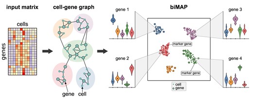
CAbiNet takes a gene expression matrix as input, in which genes are presented in rows and cells in columns. The algorithm builds on the transformation of the data into a matrix of Pearson residuals as done in correspondence analysis (CA). CA decomposes this matrix into a singular vector matrix of cells (matrix U in Figure 1, see also in section Correspondence analysis), a diagonal matrix with singular values and a singular vector matrix of genes (matrix V in Figure 1). Singular vectors are sorted by importance—‘inertia’ in CA—which allows for projecting the data into a lower dimensional space with the highest inertias. Notably, CA provides a scaling of U and V so as to overlay them in the same space. This gives rise to interpretable cell–cell and gene–gene distances and makes cell–gene associations possible (see section Correspondence analysis). Thus, we can create a k-nearest neighbor graph connecting both genes and cells (see Figure 1). This graph, in turn, is used to calculate the overlap among neighborhoods of nodes to generate a SNN graph.

Overview of the CAbiNet algorithm. Step 1: Following correspondence analysis practice, the gene expression matrix X gets normalized and converted into a matrix of Pearson residuals, which is then decomposed by singular value decomposition into the left (U) and right (V) singular vector matrices. Step 2: kNN-graphs are built from a dimension reduced space based on either the Euclidean distance, or, for the cell–gene/gene–cell graph, based on the association ratio (see Materials and Methods Correspondence analysis). The subgraphs are subsequently merged to form a single graph containing both cells and genes. If necessary, this graph is then pruned in order to remove spurious edges and converted to a shared nearest neighbor graph (SNN-graph). The SNN-graph is the basis of both the biclustering and the biMAP. Step 3: Detect cell–gene biclusters from the graph. Step 4: biMAP visualization which displays the biclustering results with both cells and genes. Note that the biMAP can be plotted before biclustering to give users an intuition of how many biclusters are in the data. CAbiNet allows for an interactive exploration of the data. Hovering the mouse cursor over a point displays relevant information such as the cell/gene name and the bicluster. The biMAP intuitively shows the detected marker genes of each bicluster and enables a quick annotation of biclusters. For example CD19 in bicluster 3 indicates that this bicluster consists of B cells and their marker genes.
The SNN graph serves as input to an embedding algorithm like UMAP to produce the biMAP. Since the SNN graph comprises both cells and genes, the embedding of the graph yields the joint visualization of cells and genes. The shared nearest neighborhood has been shown to be a good representation of similarity in high dimensional space for gene expression data (18). Genes that are specifically highly expressed in a group of cells will therefore gravitate towards this cluster, while genes with constant expression profiles will be located close to the center of the embedding. By highlighting cell type marker genes, the biMAP can be used to quickly and easily annotate cell clusters or to identify marker genes through interactive exploration of the data.
The cell–gene graph also immediately suggests an intuitive strategy for biclustering: established clustering algorithms for large networks such as Leiden (20) or Spectral clustering (21,37,38) can co-cluster cells and genes in the SNN graph. A cluster can then contain both cells and genes, where, due to the design of the graph, genes that co-cluster with a set of cells tend to be more highly expressed in the cells they cluster with compared to other cells. We call those genes ‘associated to’ or ‘specific for’ the cells in the same cluster. The co-clusters can easily be understood as cell clusters with their corresponding marker genes. Conveniently, we can further adopt the concept of Sα-scores from Association Plots (17) to rank genes by how specific they are for a cluster.
CAbiNet is implemented as an R package and can be installed from GitHub (https://github.com/VingronLab/CAbiNet). CAbiNet functions can replace corresponding procedures in routine scRNA-seq analysis piplines and are compatible with Bioconductor’s SingleCellExperiment object. The package will produce a biMAP with cells and genes colored according to the biclustering result. CAbiNet also allows for highlighting genes of interest in either a static or interactive biMAP. This promotes an intuitive exploration of genes and cells and facilitates cell type annotation. The Online Supplementary Material of this paper contains interactive html-files of biMAPs for the data sets discussed below. Users can mouse over the points in the biMAP to see the information of items including types (cell/gene), names and assigned biclusters of the points.
Analysing scRNA-seq data with CAbiNet: PBMC10x data
We demonstrate the basic functionality of CAbiNet with a single-cell Peripheral Blood Mononuclear Cell (PBMC10x) RNA-seq data set (34). This data set comprises 3176 cells annotated into nine cell types with 11 881 expressed genes detected. For our purpose, the advantage of this data set is that the authors have provided expert annotation of cells based on FACS. Among others, the nine annotated cell types include B cells, CD14+ monocytes, and natural killer cells.
As described above, CAbiNet performs dimensionality reduction, clustering and visualization. After standard pre-processing (Materials and Methods: Data Pre-processing), CAbiNet computes CA, projects the PBMC10x data into a lower dimensional space and builds the SNN graph. CAbiNet then detects the biclusters and visualizes the results in a biMAP (Figure 2A) by applying UMAP on the SNN graph.
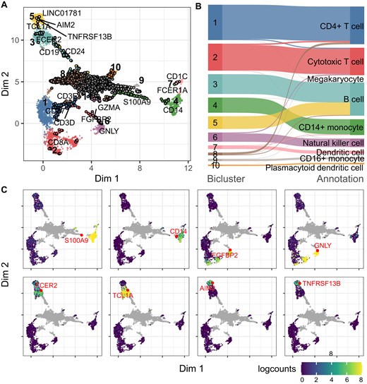
Application of CAbiNet on PBMC10x data. (A) Joint biMAP visualization of the cell–gene biclustering results by CAbiNet, with genes and cells from the same bicluster colored identically. Genes are black circles filled in with the color of the associated cell cluster and cells are smaller dots. Some known marker genes have been labeled manually. An interactive version of this Figure can be found in the Supplementary Data. (B) The agreement between the expert annotation and CAbiNet biclustering results is shown in the Sankey plot. (C) The expression levels and position of selected marker genes are shown on the biMAP. The grey points are genes and cells are colored by the log2-expression levels of genes highlighted in red. CD14+ monocytes marker genes S100A9 and CD14 in bicluster 4 are highly expressed in cells that co-clustered with them. The natural killer cells marker genes FGFBP2 and GNLY are highly expressed in the co-clustered cells in bicluster 6. FCER2 and TCL1A are highly expressed in bicluster 3, while AIM2 and TNFRSF13B are highly expressed in bicluster 5, indicating that cells in these two clusters are different B cell subtypes.
The clustering quality is commonly measured by the adjusted Rand index (ARI, see Materials and Methods: Evaluation criteria). CAbiNet achieves an ARI of 0.79 on this data set, indicating a good agreement between the CAbiNet clustering and the expert annotation. Figure 2B shows a Sankey plot illustrating the correspondence between annotation and computed clusters. The large agreement allows us to compare our results with the expert annotations.
The biMAP in Figure 2A shows clusters of cells and genes, the latter represented by black circles filled in with the color of the associated cell cluster. The clusters located in the center of the biMAP (clusters 11 and 12) are composed exclusively of genes, which are not specific to any cell cluster. Supplementary Figure S3 shows that these genes are ubiquitously expressed among cell types. As such they do not contribute information towards cluster annotation.
The biMAP places cell-type specific genes close to the corresponding cell groups. We manually labeled known marker genes for cell types to allow for easier interpretation and validation. For example, S100A9 and CD14 are located towards cluster 4 (Figure 2A) and are known marker genes for CD14+ Monocytes, immediately suggesting that cluster 4 corresponds to this cell type. The feature plots in Figure 2C confirm that indeed these two marker genes are highly expressed in this cluster. The Sankey plot in Figure 2B also confirms the identity of cluster 4 as CD14+ monocytes. Likewise, the natural killer cell marker genes FGFBP2 and GNLY are close to cluster 6, suggesting the identity for this cell cluster, which is also supported by their expression pattern in the feature plots (Figure 2C) and by the mapping to the expert annotation in the Sankey plot (Figure 2B).
Interestingly, the biMAP suggests a separation among the expert annotated B cells into two groups represented by the two clusters numbered 3 and 5 in Figure 2A and B. Each of the two subgroups has its own set of marker genes. Note that the color code for the genes coincides with that of the cells from the same cluster. Cluster 3 in cyan-blue appears to be naive B cells based on the proximity to naive B cell marker genes FCER2 and TCL1A (Figure 2A) (39). Likewise, genes AIM2 and TNFRSF13B belong to cluster 5 (light-yellow color) and their association with memory B cells (39,40) suggests this identity for cluster 5 (Figure 2A). The gene expression levels shown in the feature plot in Figure 2C support this interpretation.
We also illustrate the capability of CAbiNet in distinguishing sub-cell types with tabula muris limb muscle data set, when gene pruning is applied to remove redundant house-keeping genes (see Supplementary Material and Supplementary Figures S1 and S2).
CAbiNet correctly clusters developmental trajectories in cerebral organoids
In order to test the performance of CAbiNet on a highly complex data set, we analyzed a scRNA-seq data set comprising 35 291 cells derived from human cerebral organoids (abbrv.: brain organoids) (22). The data is of particular interest as it consists of fully differentiated neurons, undifferentiated neural stem cells, as well as cells in transitory states which can have a considerable overlap in their expression profiles. This data set thereby helps to highlight the capabilities and limitations of CAbiNet. For a detailed description of the data and the processing see Materials and Methods Human cerebral organoids data.
CAbiNet groups the organoids into 13 clusters (Figure 3A). The Sankey plot in Figure 3D shows that the biclusters overlap well with the 17 annotated cell types from the original publication (22) (ARI: 0.57). As can be observed in Figure 3A, the biMAP embedding divides the data into two major parts: The stem cells in the lower half, and more specialized cell types in the upper part. Additionally, cortical cell types are located on the left side while cell types towards the upper right belong to non-neural lineages. Furthermore, a clear developmental trajectory can be observed from the cortical neural stem cells (NSCs) expressing SOX9, towards cortical neurons via intermediate progenitors (IPs) (Figure 3A, B). Clusters 1, 6 and 7 consist of NSCs in different stages of the cell cycle (Supplementary Figure S5), with cells from cluster 7 comprised of dividing cells. Marker genes associated with differentiating neurons (NEUROG2) are situated in close proximity to cluster 4 (IPs), while markers for postmitotic cortical neurons (NEUROD2, NEUROD6) are embedded adjacent to the terminally differentiated cells (cluster 2) (Figure 3A, B, Supplementary Figure S4A). Clusters 2, 3 and 4 have a large overlap in their expression profiles, but cells from cluster 3 co-cluster with genes more associated with regions of the midbrain/thalamus such as FOXP2 and TCF7L2 (Supplementary Figure S4B-C). Cluster 3 can be further subdivided by their co-clustered genes into two subpopulations: GABAergic inhibitory neurons (LHX1, GAD1) and excitatory glutamatergic neurons (ADCYAP1, SLC17A6, see Supplementary Figure S4D–G). The myelination factors MPZ and EGR2 are embedded together with cluster 10, indicating that the cluster consists of Schwann cells (Supplementary Figure S4H, I). This is further confirmed by the co-embedding of SOX10, which has been shown to be required to maintain the Schwann cell identity (41) (Supplementary Figure S4J). Cells from cluster 13 are characterized by strong expression of NEUROD1, PPP1R17, ISL1, POU4F1 and SIX1, all of which are embedded within the cluster (Supplementary Figure S4K–O). NEUROD1, ISL1, POU4F1 (the gene producing BRN3A) and SIX1 have been shown to play vital roles in sensory neuron development (42–45) whereas PPP1R17 is a typical Purkinje cell marker (46). This makes it difficult to assign a specific cell type to the cluster. Accordingly, the cells were labelled as ‘posterior CNS/PNS’ cells in the original publication.
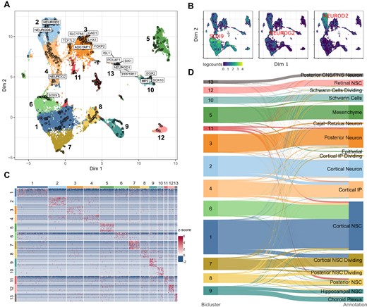
CAbiNet correctly clusters developmental trajectories in cerebral organoids. (A) biMAP of the brain organoid data set colored by CAbiNet biclusters. Marker genes discussed in the main text for specific brain regions and neuronal cell types are marked. An interactive version of the biMAP is available for download in the Supplementary Data. (B) The feature plots highlight the placement of marker genes along the developmental trajectory from neural stem cell (SOX9) to IPs (NEUROG2) to fully differentiated neurons (NEUROD2). (C) Heatmap showing the top 10 genes with the highest Sα-score per cluster. (D) The Sankey plot illustrates how the cell clusters relate to the expert annotations. The cell types are colored by the cluster that contains the largest number of cells from the cell type.
As shown in the heatmap in Figure 3C, the top 10 co-clustered genes show distinct expression patterns and are consistently more highly expressed in their respective cluster. This shows that the biclustering indeed recovers relevant marker genes.
CAbiNet constructs clusters consistent with spatial dimensions in Drosophila melanogaster spatial transcriptomics embryo data
Spatial transcriptomic data constitutes a particular challenge to the data analysis due to the large number of drop-outs (23,47). To further study the performance of CAbiNet on such sparse data, we applied it to spatial transcriptomic data of Drosophila melanogaster late-stage embryos (14–16 h after egg laying (E14-16h)) (23). The gene expression profile was resolved by Stereo-seq (47) yielding 14 808 pseudo-cells (bins of pixels on a chip which are recognized as equivalent to cells by the original publication) with 7178 genes. In the original publication 10 cell types were annotated based on unsupervised clustering. The standard UMAP projection shown in Figure 4A illustrates that the boundaries between cell types are ill defined (e.g. epidermis versus foregut and epidermis versus trachea). This highlights the difficulty of distinguishing cell types and identifying corresponding marker genes in spatial scRNA-seq data.
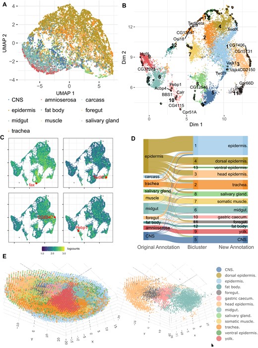
CAbiNet constructs clusters consistent with spatial dimensions in D. melanogaster Stereo-seq data. (A) UMAP embedding of expert annotated cell types. (B) biMAP embedding of cell–gene biclusters. The genes and cells from the same biclusters are colored identically. Genes are filled circles with a black outline and the cells are the smaller dots. Selected marker genes are labeled in the biMAP. (C) The feature-biMAPs show the expression levels of known marker genes (fax (CNS), TwldC (foregut), CG6347 (head epidermis) and Pebp1 (gastric caecum)) in the cells. The cells are colored by the log2-expression levels of the highlighted genes. (D) The Sankey plot shows the consistency among the expert annotation, the biclustering results from CAbiNet and the revised CAbiNet-based annotations. (E) Spatial distribution of the cells. The left panel is the 3D visualization of the embryo with cells colored by the biclustering. The right panel shows four cell types out of the left panel. From head to tail they are head epidermis, foregut, gastric caecum and midgut. Interactive versions of panel b and e can be found in the Supplementary Material.
CAbiNet recognizes 13 biclusters from the data with biologically meaningful co-clustered marker genes. For example, 12 out of 15 genes (fax, Bacc, Cam, Gbeta13F, 14-3-3ε, fabp, His4r, HmgZ, CG41128, ps, smt3, arm) in cluster 5 are known marker genes of the central nervous system (CNS), and 7 out of 12 genes (TwdlC, CG12164, Cpr50Cb, Cpr56F, Cpr65Av, Cpr66D, CG13043) in cluster 11 are known foregut marker genes. The expression levels of fax and TwdlC shown in Figure 4C suggest that they are specifically highly expressed marker genes for the co-clustered cells.
CAbiNet also captures fine-grained cluster structure and offers an intuitive embedding of biclusters which can be used for cell type annotation. For example, we found that most cells annotated as midgut in the original publication using Scanpy correlate to two clusters by CAbiNet, cluster 6 and 10, which are recognizable as distinct groups in the biMAP (Figure 4B, D). This indicates that cells originally annotated as midgut could be further divided into two cell types. Checking the detected marker genes in cluster 10, we found some of them, e.g. Pebp1 and Acbp4, are known marker genes of gastric caecum. These genes have overall higher expression levels in cluster 10 compared to other clusters (Figure 4C), indicating that cells in cluster 10 represent gastric caecum, a sub-structure of the midgut that was not previously identified in the original analysis. Similarly, we also found that cluster 3 represents head epidermis which is a subtype of epidermis. The expression level of head epidermis marker gene CG6347 is shown in Figure 4C.
Based on the biclustering results from CAbiNet, we generated new annotations of the cell clusters. The annotated cell types are shown in Figure 4D. Figure 4E shows the cells in the embryo, color-coded by these improved annotations. Reminiscent of the actual embryonic anatomy, the spatial positions of annotated head epidermis, foregut, gastric caecum and midgut cells (right panel of Figure 4E) are ordered from head to tail.
Thus, CAbiNet provides a more informative joint embedding of genes and cells compared to Figure 4A. CAbiNet also generates fine-grained biclustering results and supports cell type annotation for spatial transcriptomic data.
Evaluation on simulated data
In order to determine how well the biclustering performs on scRNA-seq data, we ran CAbiNet as well as nine other biclustering algorithms on simulated data generated using Splatter based on two real scRNA-seq data sets (25) (see Materials and Methods Splatter simulated data). Splatter can learn and preserve the distribution patterns from real data and generate simulated scRNA-seq data with well separated cell clusters and corresponding differentially expressed genes. Twelve simulated data sets were generated with different parameters based on two real scRNA-seq data sets to cover different clustering difficulties (see Table 1). Since the clusters and their differentially expressed genes are known, one has a gold-standard biclustering to compare computational results to. The heatmaps of the the simulated data sets in Supplementary Figure S8 show the bicluster structure of the data and give a visual indication of how difficult the (bi-)clustering task on a data set is.
We tested the CAbiNet implementation with both Leiden and Spectral clustering and compared to QUBIC (5), s4vd (9), Plaid (48), Unibic (6), BiMax (7), CCA (4), Xmotifs (8), IRIS-FGM (QUBIC2) (12,49), BackSPIN (10) and DivBiclust (13). Some of the algorithms identify hard cell–gene biclusters, while others recognize overlapping clusters. Although DivBiclust is a biclustering-based framework, it only outputs cell clusters. We therefore only evaluated its cell clustering performance. A brief summary of the characteristics of algorithms can be found in Supplementary Table S1. In order to better compare CAbiNet to popular scRNA-seq analysis workflows, we clustered cells and identified differentially expressed genes with two R packages, Monocle3 (50) and Seurat (51). We treated genes that are differentially expressed as if they were co-clustered with the cells from the respective cluster (see Materials and Methods section Benchmarking).
To be fair to all the methods, we tested numerous parameter choices throughout an algorithm’s range. For the summary statistics we ran every algorithm with 108 different parameter combinations that were chosen individually for each algorithm and are intended to represent the capabilities of the algorithm well.
To compare the time consumption of the algorithms, the running time of each run is recorded. CAbiNet is shown to run similarly fast as 7 out of 12 (bi-)clustering algorithms that have been compared with (Figure 5D). CAbiNet is slower than CCA, QUBIC and DivBiclust, but is faster than IRISFGM and BackSPIN which are the only biclustering algorithms developed for scRNA-seq data analysis. Compared with IRISFGM and BackSPIN, CAbiNet is more capable to deal with large-scale scRNA-seq and spatial transcriptomic data sets.
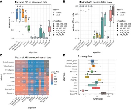
Benchmarking of CAbiNet biclustering against other biclustering algorithms and scRNA-seq analysis toolkits. (A) Maximal clustering error (CE) of biclusters detected from simulated data sets over all parameter choices. Different simulation parameters (the clustering ‘difficulty’) are differentiated by shape, whereas the data set used to estimate the base parameters (zeisel and pbmc3k) is marked by different shades of grey. (B) Maximal adjusted Rand index (ARI) of the obtained cell clusters for the (bi-)clustering results over all parameter choices for each algorithm on simulated scRNA-seq data sets and (C) experimental scRNA-seq data. An ARI of 1 indicates a perfect match between detected clusters and ground-truth. An ARI of 0 indicates a random clustering, whereas negative values indicate a clustering worse than what would be expected from a random labeling. If all runs failed (crashed) or returned nonsensical results they are labeled as N/A. (D) The running time across all parameter choices for all simulated data sets. To improve readability, the algorithms Bimax and Xmotifs are not shown in panels A–D due to being uninformative, i.e. the ARI and CE scores are consistently around 0. Their average performance is shown in Supplementary Figure S7 in the Supplementary Materials.
The scalability of CAbiNet was evaluated using simulated data sets consisting of 2000 genes and varying cell counts ranging from 1000 to 80 000 cells. The Supplementary Material provides detailed information on these tests. The results are depicted in Supplementary Figure S9. With 16 threads, CAbiNet takes about 50 min to cluster the large dataset containing 80 000 cells. However, memory requirements for large data sets are substantial. For more than 100 000 cells and 2000 genes it is recommended to have more than 1TB of RAM available.
Performance of algorithms in terms of clustering quality was evaluated by the adjusted Rand index (ARI) and clustering error (CE) metrics (27,28) (see Materials and Methods section Evaluation criteria). The ARI provides a quantitative comparison between detected cell clusters and the ground-truth clusters. The CE measures the similarity between detected and annotated biclusters. For both measurements a higher score indicates a better (bi-)clustering. To account for the uncertainty in parameter choice, biclustering quality of algorithmic results is benchmarked firstly by the maximal achievable values of CE and ARI (Figure 5A, B) and secondly by the average values (see Supplementary Figure S7 in Supplementary Materials) over all runs on each data set.
CAbiNet achieves the highest maximal and mean CE scores on nearly all data sets when being compared with other biclustering algorithms (Figure 5A). Only BackSPIN performs marginally better than CAbiNet on a single simulated dataset when comparing the mean CE (Supplementary Figure S7B). CAbiNet is the only biclustering algorithm in the comparison that produces meaningful biclusters for the hardest simulations, while only CAbiNet together with Plaid, s4vd and BackSPIN generate meaningful biclusters for easier data sets. Although they are not biclustering algorithms in the strict sense, both Seurat and Monocle3 perform well on the simulated data. While Seurat obtains comparable or slightly better mean CE scores (Supplementary Figure S7B), its achieved maximal CE results are overall lower than that of CAbiNet (Figure 5A). Monocle3 obtains mean and maximal CE scores that are consistently lower than those achieved by CAbiNet and Seurat (Figure 5A and Supplementary Figure S7B). These methods, however, do not provide a joint visualization of cells and genes.
In terms of cell clustering quality as measured by the maximal ARI, CAbiNet achieves nearly perfect clustering for all but one data set. While BackSPIN and DivBiclust are also able to achieve an ARI of 1 for a smaller number of data sets, their overall obtained maximal ARI scores are lower than CAbiNet. Similarly to CAbiNet, Seurat and Monocle3 achieve perfect cell clustering on all but the most difficult simulated data set (see Figure 5B). Monocle3 generally achieves a comparable cell clustering quality as CAbiNet on the majority of simulated and experimental data sets, but its performance seems to deteriorate with larger data sets (Figure 5B, C). Furthermore, Moncocle3 fails to return any meaningful (bi-)clusters for a considerable fraction of runs (Supplementary Figure S7C, D).
Since some biclustering algorithms (e.g. CCA, QUBIC or Unibic) were not initially developed for scRNA-seq data analysis (see Supplementary Table S1), they didn’t take the sparsity and high dropouts of scRNA-seq data into account. It is therefore expected that they are struggling to analyze scRNA-seq data. Comparing with IRISFGM and BackSPIN, which are scRNA-seq conscious biclustering algorithms, CAbiNet outperforms them on most simulated data sets. A longer discussion of the performance of the tested algorithms can be found in the Supplementary Material and Supplementary Figure S11.
We furthermore compared the robustness of CAbiNet over the choice of dimensions to two other SVD based algorithms, Seurat and Monocle3, on simulated data. As can be seen in Supplementary Figure S10, both Seurat and CAbiNet perform poorly when too few dimensions are retained. Both algorithms achieve good cell clustering results over a wide range of dimensions when the kept dimensions are more than the number of clusters in the data. In general, Seurat needs a higher number of dimensions than CAbiNet to obtain a good cell clustering on simulated data sets with six cell clusters (Supplementary Figure S10A), while a similar number of dimensions is required for both algorithms on simulated data sets with 20 clusters (Supplementary Figure S10B). Monocle3’s performance decreases when too many dimensions are picked (Supplementary Figure S10A). For data sets with 20 embedded clusters Monocle3 crashed on the majority of runs and was therefore omitted from the systematic comparison shown in Supplementary Figure S10B. For a more in depth description see also the Supplementary Materials.
Evaluation on expert annotated data
To assess the performance of CAbiNet on experimental data we tested it on nine expert annotated scRNA-seq data sets. Again, we compared CAbiNet to the same nine biclustering algorithms as above and to the cell clustering tools Seurat, Monocle3 and DivBiclust. Since the expert annotated data only provides silver-standard ground-truth of cell types and no ground-truth is available to evaluate the biclusters, the ARI of cell clusters, but not the CE of biclusters, is used as a quality measure.
The data sets range in size from 461 up to 35 291 cells and have been generated with different sequencing technologies (see section Experimental scRNA-seq data with ground truth cell types and Table 2). Similarly to the benchmarking on simulated data, we again used 108 parameter combinations for each algorithm to ensure an even playing field.
Compared to the other biclustering methods, i.e. not considering Seurat, Monocle3 and DivBiclust, CAbiNet with either Leiden or spectral clustering yields the highest maximal ARI for all data sets with the exception of the zeisel data set (highest ARI by BackSPIN, Figure 5C). CAbiNet also achieves the highest average ARI on the cell clustering for all data sets except for one (Tirosh), where Plaid achieved the highest average ARI (Supplementary Figure S7A). CAbiNet with spectral clustering performs on average slightly worse than CAbiNet with Leiden for almost all data sets (Supplementary Figure S7A). However, it still outperforms other biclustering algorithms, with the exception of Plaid on the ‘Tirosh’ data set, as measured by both the maximal and average ARIs of cell clusters. Some biclustering algorithms such as BackSPIN, Xmotifs and s4vd completely failed in detecting any cell clusters for some data sets (marked as ‘N/A’ in grey blocks in Figure 5C and Supplementary Figure S7A, B), either because of issues in the algorithms’ implementation, the ability of algorithms in dealing with large data sets, or because no biclusters were returned by the algorithm.
Comparing with the scRNA-seq cell clustering algorithms Monocle3, Seurat and DivBiclust, CAbiNet overall performs better on the majority of experimental data sets. Only on the zeisel, Tirosh and PBMC10x data sets Monocle3 and Seurat perform slightly better than CAbiNet as evaluated by the maximal ARI (Figure 5C). CAbiNet on average outperforms Monocle3 on larger data sets, while Monocle3 seems to perform slightly better on medium sized data sets (Supplementary Figure S7A). On 8/9 data sets, CAbiNet on average produces a better cell clustering than Seurat, which only outperforms CAbiNet on the Darmanis data. Similarly, CAbiNet yields a more accurate cell clustering than DivBiclust on all tested data sets (Supplementary Figure S7A). Notably, Monocle3 fails to recognize cell clusters in the DmelSpatial data set and DivBiclust fails to identify cell clusters for the largest three data sets (DmelSpatial, TabulaSapiens and BrainOrganoids), whereas CAbiNet still obtains reasonable clustering accuracy on these data sets.
Ranking the biclustering algorithms by their running time on real data sets yields similar results as for the simulated data (see Supplementary Figure S6). CAbiNet is slower than Bimax and QUBIC, but runs faster than IRISFGM, Unibic, BackSPIN and s4vd on all the tested data sets. In terms of scalability and accuracy CAbiNet is comparable with Seurat and Monocle3. CAbiNet runs faster than IRISFGM and BackSPIN, two biclustering algorithms developed for scRNA-seq data, and produces more accurate biclusters. On small and medium sized data sets, CAbiNet runs faster than Plaid, while being comparable with Plaid on large data sets.
Discussion
We introduced CAbiNet and the biMAP as a novel biclustering and visualization method to simultaneously cluster and plot cells and genes, allowing for interactive data exploration. The biMAP is a planar embedding placing cell clusters with the genes that are expressed in the co-clustered cells. It thus allows researchers to better understand cell–gene relationships and to annotate cell types easily. Although we mainly discuss CAbiNet in the context of scRNA-seq data, the method could be equally applied to bulk RNA-seq data or other data formats such as ATAC-seq.
We showed the applicability of CAbiNet to a wide variety of data sets and highlighted multiple ways in which CAbiNet can be used to generate novel insights. We demonstrated the general usage of CAbiNet to identify cell types on the PBMC10x data set. Even in highly complex data sets, such as the brain organoids or spatial Drosophila melanogaster data that include developmental trajectories, CAbiNet is able to facilitate the differentiation of sub-types based on the 2D layout of cells and co-clustered marker genes. Moreover, CAbiNet is capable of refining the cell types in the spatial data and recognizes sub-types of epidermis and differentiates gastric caecum from midgut.
CAbiNet implements a novel biclustering approach. Benchmarking on simulated data showed that CAbiNet is the best performing biclustering algorithm in comparison to a suite of established algorithms. CAbiNet is overall the best tested biclustering algorithm on the experimental scRNA-seq data sets, where it outperforms all the other biclustering algorithms on all but one data set. Comparing with the cell clustering algorithms Seurat, Monocle3 and DivBiclust, CAbiNet performs slightly better than Seurat on real data, while both achieve an ARI of 1 on all but one simulated data set. CAbiNet and Monocle3 have comparable performance on both simulated and small-sized real data sets, while Monocle3 performed worse on large-sized real data. In a real application without knowledge of the true clustering, the visual representation of genes and cell clusters in the biMAP provides additional information as to the reliability of a clustering and its marker genes.
An inherent limitation of CAbiNet is that it can only detect upregulated genes. The method is insensitive to genes which are characteristically downregulated in a certain cell cluster. However, as cell types are generally defined through the expression and not the absence of specific genes, this is hardly an obstacle to cell type annotation. Compared to the other tested scRNA-seq biclustering algorithms IRISFGM and BackSPIN, CAbiNet yields higher accuracy biclusters at a lower running time. However, due to the fact CAbiNet includes both cells and genes in the graph the computational load increases significantly when a large number of genes is included. Although we have ameliorated the problem by including a feature selection procedure, there is probably still room to improve the implementation of CAbiNet.
CAbiNet assigns each gene to one particular cluster in which it is specifically expressed. This hard clustering of genes is beneficial for cell type annotation and the differentiation of sub-cell types, but in some cases marker genes that are in fact shared between two clusters could be assigned to a single cluster.
Therefore, a potential improvement for future development would be to allow for a soft assignment of genes to clusters. This would provide a more realistic representation of genes that are involved in several cell types.
Conclusion
CAbiNet presents clustered cells together with their marker genes, thus providing key insight into a single-cell transciptomic data set. Based on experimental data sets from diverse biological contexts and with distinct properties, we showed how CAbiNet improves over other clustering algorithms, aids in annotating cell types and visualizes the results. Our benchmarking results demonstrate that CAbiNet outperforms other biclustering algorithms on simulated and real scRNA-seq data, making it an important addition to the tool set available to researchers. Visualizing cells and genes simultaneously in a biMAP enables researchers to succinctly communicate their results and to uncover previously hidden cell–gene relationships in the data. CAbiNet can be easily integrated into common workflows where it can be used in tandem with other tools or replace repetitive analysis steps during cell type annotation.
Data availability
The simulated data sets we generated and the experimental data sets we used can be downloaded from Zenodo (https://zenodo.org/records/10260709 and https://zenodo.org/records/10932001). Raw experimental data sets were sourced from the references listed in Table 2.
Code availability
The CAbiNet package can be installed from GitHub (https://github.com/VingronLab/CAbiNet). The source code can also be found on figshare https://figshare.com/articles/software/CAbiNet_Joint_clustering_and_visualization_of_cells_and_ genes_for_single-cell_transcriptomics/23276402 and GitHub (https://github.com/VingronLab/CAbiNet_paper).
Supplementary data
Supplementary Data are available at NAR Online.
Acknowledgements
The authors wish to thank Helene Kretzmer for her valuable feedback on the manuscript and the IT group of the Max Planck Institute for Molecular Genetics for maintaining the computational resources in house and for their support.
Funding
C.K. gratefully acknowledges financial support by the IMPRS-BAC PhD program; Y.Z. gratefully acknowledges partial support by Shenzhen Science and Technology Program [KQTD 20180411143432337, China]; M.V. gratefully acknowledges many helpful discussions during the program ‘Computational Innovation and Data-Driven Biology’ of the Simons Institute for Theory of Computing at Berkeley; Y.H. and Q.H. acknowledge support by Shenzhen Key Laboratory of Gene Regulation and Systems Biology [ZDSYS 20200811144002008, China to Y.H.]; National Natural Science Foundation of China [82373975 to Y.H., 32100684 to Q.H.]. Funding for open access charge: Max Planck Society.
Conflict of interest statement. None declared.
References
Author notes
The first two authors should be regarded as Joint First Authors.

Comments