


ABSTRACT
We cross-correlate positions of galaxies measured in data from the first three years of the Dark Energy Survey with Compton-y maps generated using data from the South Pole Telescope (SPT) and the Planck mission. We model this cross-correlation measurement together with the galaxy autocorrelation to constrain the distribution of gas in the Universe. We measure the hydrostatic mass bias or, equivalently, the mean halo bias-weighted electron pressure 〈bhPe 〉, using large-scale information. We find 〈bhPe 〉 to be |$[0.16^{+0.03}_{-0.04},0.28^{+0.04}_{-0.05},0.45^{+0.06}_{-0.10},0.54^{+0.08}_{-0.07},0.61^{+0.08}_{-0.06},0.63^{+0.07}_{-0.08}]$| meV cm−3 at redshifts z ∼ [0.30, 0.46, 0.62, 0.77, 0.89, 0.97]. These values are consistent with previous work where measurements exist in the redshift range. We also constrain the mean gas profile using small-scale information, enabled by the high-resolution of the SPT data. We compare our measurements to different parametrized profiles based on the cosmo-OWLS hydrodynamical simulations. We find that our data are consistent with the simulation that assumes an AGN heating temperature of 108.5 K but are incompatible with the model that assumes an AGN heating temperature of 108.0 K. These comparisons indicate that the data prefer a higher value of electron pressure than the simulations within r500c of the galaxies’ haloes.
1 INTRODUCTION
In the canonical cold dark matter paradigm, dark matter collapses non-linearly to form gravitationally bound haloes. These dark matter haloes host the visible baryonic matter, dominantly in the form of stars and hot gas. The interactions of these three components – dark matter, stars, and gas – are critical for understanding the astrophysical processes that govern galaxy formation and evolution (see Naab & Ostriker 2017, for a review). Constraining these astrophysical processes is also one of the main focuses in galaxy surveys today (Semboloni, Hoekstra & Schaye 2013; Eifler et al. 2015; Chisari et al. 2019; Huang et al. 2019; Chen et al. 2023), as astrophysical uncertainties are becoming the limiting factor for cosmological analyses.
The joint analysis of observations at optical/near-infrared and microwave wavelengths provides an emerging opportunity to study the connection between gas, stars (which form the visible part of the galaxies), and dark matter. Surveys at optical/near-infrared wavelengths precisely measure the locations and properties of hundreds of millions of galaxies. On the other hand, at microwave wavelengths, the thermal Sunyaev–Zeldovich effect (tSZ; Sunyaev & Zeldovich 1972), which arises from the inverse-Compton scattering of cosmic microwave background (CMB) photons with high-energy electrons, effectively traces the distribution of hot gas in the Universe. The amplitude of this effect depends on the average thermal pressure profile of galaxy groups and clusters (Battaglia et al. 2012; Bhattacharya et al. 2012). The observable quantity of the tSZ effect is usually measured via the Compton-y parameter, which we will refer to as y throughout this paper. As shown in Hill et al. (2018) and Pandey et al. (2019), on large scales, the cross-correlations between galaxies and maps of y can constrain the thermal energy content of the Universe. In addition, Schaan et al. (2021) showed that the small-scale information of the galaxy-y correlation further constrains the gas thermodynamics and the properties of astrophysical feedback processes. On the practical side, these cross-correlation measurements are very robust to systematic effects, as the two data sets are almost completely independent and experimental systematic effects that only reside in one data set will not bias our final measurement. The robustness of these cross-correlation measurements makes them very attractive as we approach an era where observational cosmology is increasingly systematics limited.
Most recent analyses have focused on constraining the thermodynamics of intergalactic gas through measurements of the quantity 〈bhPe〉, often referred to as the halo bias-weighted mean electron pressure.1 This quantity is interesting for two reasons: (i) it directly probes the mean electron pressure of the Universe and the growth of structure, (ii) it is the direct observable of the SZ-galaxy cross-correlation at large scales (Vikram, Lidz & Jain 2017). Some of these analyses then rely on the halo model to obtain the so-called hydrostatic bias (or mass bias), usually denoted bH (Vikram et al. 2017; Pandey et al. 2019; Koukoufilippas et al. 2020; Yan et al. 2021).
Three previous studies have combined the galaxy-y cross-correlation with the the galaxy–galaxy autocorrelation (Vikram et al. 2017; Pandey et al. 2019; Koukoufilippas et al. 2020). All three of these studies focused mainly on the Planck MILCA y-map (Planck Collaboration XIII 2016a) but used different galaxy samples: Vikram et al. (2017) used the group catalogue from SDSS produced by Yang et al. (2007) (halo mass 1011–1015 M|$_{\odot }\, h^{-1}$|, redshift range 0.01–0.2); Pandey et al. (2019) used DES redmagic galaxies from Rozo et al. (2016) (halo mass ∼ 1013 M|$_{\odot }\, h^{-1}$|, redshift range 0.15–0.75), and Koukoufilippas et al. (2020) used a combination of 2MASS (Bilicki et al. 2014) and WISE × SuperCOSMOS (Bilicki et al. 2016) galaxies (halo mass ∼1012–1013 M|$_{\odot }\, h^{-1}$|, redshift range <0.4). The first two measurements were carried out in real-space while the last one used a harmonic-space estimator. The combination of the galaxy-y cross-correlation and the galaxy autocorrelation breaks the degeneracy between 〈bhPe〉 and the galaxy bias. All three analyses show consistent results, albeit with large uncertainties.
Focusing mainly on the MILCA y-map, Yan et al. (2021) took a different approach and combined the galaxy-y cross-correlation and cross-correlation of galaxy and CMB lensing, arguing that a pure cross-correlation analysis is less prone to systematic effects. The galaxy sample used is the weak lensing sample in the KiDS-1000 data set (halo mass |$\sim 10^{12}\!-\!10^{15} \, \mathrm{M}_{\odot }\, h^{-1}$|, redshift <1).
Chiang et al. (2020) explored a rather different route by using the individual temperature maps from different frequencies in Planck instead of using a y-map. They cross-correlate these maps with spectroscopic galaxies in SDSS spanning a large range in mass and redshift (halo mass |$\sim 10^{11.5}\!-\!10^{13.5} \, \mathrm{M}_{\odot }\, h^{-1}$|, redshift <3). The cross-correlation amplitudes of the different maps at a given redshift effectively gives a Spectral Energy Distribution (SED), which the authors fit to a combination of the tSZ and cosmic infrared background (CIB) SEDs. The result from this multichannel SED fitting approach can directly be translated into 〈bhPe〉. Chiang et al. (2020) showed that this procedure yields less CIB contamination at high redshift than using the y-maps directly.
All the aforementioned analyses rely mainly on large-scale information, as they are limited by the resolution of the Planck maps at ∼10 arcmin. With the help of high-resolution y-maps from ongoing CMB experiments, we are starting to explore the gas distributions on smaller scales. Schaan et al. (2021) cross-correlated the cmass (mean redshift 〈z〉 = 0.55, mean virial mass 〈Mvir〉 = 2.1 × 10¹³ M|$_{\odot }\, h^{-1}$|), and lowz (〈z〉 = 0.31, 〈Mvir〉 = 3.5 × 10¹³ M|$_{\odot }\, h^{-1}$|) samples from Baryon Oscillation Spectroscopic Survey (BOSS; Dawson et al. 2013) DR10 and DR12 with the y-map constructed by combining Atacama Cosmology Telescope (ACT; Swetz et al. 2011) DR5 and Planck data (Planck Collaboration XIII 2016a). The tSZ profiles were measured at high significance within the size of a typical halo. Amodeo et al. (2021) compared these measured profiles to those in hydrodynamical simulations and found the measured profiles to disagree with simulations especially at large radii – the data shows a peakier profile in general. This could suggest that the subgrid stellar and AGN feedback models in these simulations do not sufficiently heat the gas in the outer regions. Gatti et al. (2022) and Pandey et al. (2022) recently performed a cross-correlation of galaxy weak lensing with the ACT DR4 tSZ maps. They showed that, when using the gas model in Le Brun, McCarthy & Melin (2015), the shear-y measurements slightly prefer a stronger AGN feedback model than cosmic-shear-only analyses. Tröster et al. (2022) also found that shear-y prefers a stronger AGN feedback than cosmic shear (Tröster et al. 2021). Other constraints on small-scale baryonic effects on cosmic shear measurements include Yoon & Jee (2021), Huang et al. (2021), Chen, Zhang & Yang (2022), Chen et al. (2023), and Schneider et al. (2022).
Building on past work (e.g. Vikram et al. 2017; Pandey et al. 2019; Koukoufilippas et al. 2020), we measure and model two sets of correlation functions: galaxy clustering, ‘gg’, and the galaxy-y, ‘gy’ cross-correlation. We use a galaxy sample defined for the recent large-scale structure cosmology analysis from the Dark Energy Survey (DES; DES Collaboration 2022) the maglim galaxies, the MILCA y-maps from Planck Collaboration XIII (2016a), as well as y-maps constructed using a combination of South Pole Telescope (SPT) and Planck data from Bleem et al. (2022). In particular, the cross-correlations between DES galaxies and SPT-SZ + Planck y-maps have several advantages relative to previous analyses: (1) the galaxies are well-characterized and vetted for observational systematics; (2) the galaxies span a large redshift range (up to z ∼ 1) with good statistics reaching small scales; (3) the y-map has lower noise and higher resolution compared to y-maps produced using Planck data only. Finally, as this galaxy sample is used for cosmological analyses in DES, our results can help constrain astrophysical nuisance parameters and improve cosmological constraints from DES. We first look at the two-halo regime (large-scales) to constrain 〈bhPe〉 and compare with previous work. We then look into the one-halo regime to map the gas profile around galaxies in our sample. We note also that our galaxy sample has been extensively characterized via galaxy–galaxy lensing in an HOD analysis (Zacharegkas et al. 2022) and has been determined to have an average halo mass of a few times 1013 M|$_{\odot }\, h^{-1}$|.
This paper is structured as follows. In Section 2 we describe the theoretical prescription used to model the distributions of galaxies and gas. In Section 3 we describe the galaxy and y-maps that we use in this analysis. In Section 4 we describe our analysis prescription including our covariance matrix, scale cuts, likelihood inference, and systematic tests. In Section 5 we discuss our constraints on the hydrostatic mass bias using large-scale information, and in Section 6 we discuss our constraints on gas profiles using small-scale information. We conclude in Section 7.
2 THEORY
The goal of this analysis is to use the HOD framework to model the angular galaxy–galaxy autospectrum |$C^{\rm gg}_{\ell }$| and the galaxy-y cross spectrum |$C^{\rm gy}_{\ell }$|. This requires a number of components that we detail in the following subsections: (1) the 3D galaxy autospectrum and galaxy-y cross spectrum following the Halo Model framework (Section 2.1); (2) an HOD model that describes how galaxies are associated with haloes (Section 2.2); (3) a functional form for the electron pressure profile around galaxies (Section 2.3); and (4) projecting the 3D galaxy–galaxy and galaxy-y cross spectrum to 2D where our measurements are made, while incorporating a number of observational systematic effects (Section 2.4).
Throughout, we will use |$\delta _{g}(\hat{n})$| to represent the projected galaxy density and |$y(\hat{n})$| to represent the y signal at a given direction |$\hat{n}$|. The projected galaxy density can be expressed as,
where ng(z) is the normalized redshift distribution of the galaxies that integrates to unity, χ(z) the comoving distance at redshift z, and Δg is the 3D overdensity of number of galaxies. The y signal is expressed as,
where σT is the Thomson scattering cross-section, me the electron mass, and Pe = neTe is the electron pressure.
Unless explicitly stated, during this study we use the best-fitting cosmological parameters from Planck (Planck Collaboration VI 2020): Ωc = 0.2607, Ωb = 0.0489, h = 0.6766, ns = 0.9665, and σ8 = 0.8102. We choose to adopt this cosmology to make comparisons with previous analyses; we have verified that changing to the DES Y3 cosmology (DES Collaboration 2022) does not alter the main conclusions of this paper.
2.1 Halo model
We describe the 3D galaxy autospectrum and galaxy-y cross spectrum using the halo model (see Peacock & Smith 2000; Seljak 2000; and references therein). Both power spectra include two contributions: the 1-halo term, P1h(k), which describes the distribution of galaxies or y inside a halo; and the 2-halo term, P2h(k), which describes the spatial distribution of the haloes themselves. The profiles are described in Fourier space, and therefore are functions of the Fourier modes k instead of radius r. For each two sets of observables u and v (which could be dark matter m, galaxy density δg, or tSZ y), we assume that their radial distribution inside the halo follow the profiles U(r|M) and V(r|M), where M is the halo mass and r is the distance from the halo centre. Their profiles in Fourier space, assuming isotropy, can be written as,
We can then write the cross power spectrum of the two observables, Puv(k), using the halo model as follows:
with
where 〈…〉 denote the ensemble average, and
where
Here, bh is the halo bias, |$\frac{{\rm d}n}{{\rm d}M}$| is the halo mass function, and PL(k) is the linear matter power spectrum. We use the halo mass function from Tinker et al. (2010), and the linear power spectrum from CAMB (Lewis, Challinor & Lasenby 2000).
In order to correct for inaccuracies in the 1-to-2-halo transition (Mead et al. 2015), we follow Koukoufilippas et al. (2020), Nicola et al. (2020) and modify the halo model power spectrum by multiplying it by the scale-dependent ratio,
where PHaloFit(k) is the HaloFit power spectrum from Takahashi et al. (2012) and PHaloModel(k) is the halo model matter power spectrum described in this section, i.e. equation (4) assuming that the observable is dark matter. Thus, the final 3D power spectra for both the galaxy autospectrum and the galaxy-y cross spectrum take the form
where u = v = δg for the galaxy autospectrum and u = δg, v = y for galaxy-y cross spectrum. We will drop the super script ‘final’ for the remainder of this text for simplicity.
2.2 Halo occupation distribution modelling
In order to model galaxy density profiles, we use an HOD model (Peacock & Smith 2000; Berlind & Weinberg 2002; Cooray & Sheth 2002; Zheng et al. 2005). In this model, dark matter haloes are populated by central and satellite galaxies. We assume that central galaxies follow a Bernouilli distribution while satellites follow a Poisson distribution (van den Bosch et al. 2013). Typically, the halo radii are defined as the size of a sphere containing a mass MΔ,
We follow previous works (e.g. Arnaud et al. 2010; Planck Collaboration XIII 2016b; Bolliet et al. 2018; Koukoufilippas et al. 2020) and choose ρ* = ρc and Δ = 500 following the rederived concentration–mass relation from Duffy et al. (2008):
with |$M_{\rm pivot}=2.7 \times 10^{12} \, \mathrm{M}_{\odot }$| and (A, B, C) = (3.67, −0.0903, −0.51).
In our HOD model, the average number of central galaxies for a halo of mass M is modelled as:
where Mmin corresponds to the characteristic minimum mass of haloes, and σlnM is the halo mass dispersion. Assuming that the halo can only form satellites if its mass is larger than a certain threshold, M0, the average number of satellites can be described as:
Following Ando, Benoit-Lévy & Komatsu (2018), Koukoufilippas et al. (2020) we choose Mmin = M0. As a consequence, all haloes containing one or more satellites contain one central, located at the centre of its parent halo.
For the satellites, we use the parametrization from Ando et al. (2018) where the satellite galaxies follow a NFW profile (Navarro, Frenk & White 1996) with a characteristic scale radius βg, up to a maximum radius βmax:
2.3 tSZ gas profile
For the electron pressure profile, we use a generalized NFW (GNFW) profile (Nagai, Kravtsov & Vikhlinin 2007; Arnaud et al. 2010). In real space, it takes the form:
where the GNFW form factor, p(r/r500c), is:
We choose the initial values (α, β, γ, cP) = (1.33, 4.13, 0.31, 1.81) as found by Planck Collaboration XVI (2013). In parts of our analysis, we allow these parameters to float in our fits, which allows us to extract additional information about the gas profile. The normalization parameter P* is:
with P0 = 6.41 the normalization constant, |$h_{70} = H_{0}/(70 \, \rm {km \, s^{-1} \, Mpc^{-1}})$|, and bH is the so-called hydrostatic mass bias, which corresponds to the fractional bias in the inferred mass using a gas proxy, assuming hydrostatic equilibrium with respect to its true mass. In the literature, this quantity is often expressed in terms of |$B=\frac{1}{1-b_{H}}$|. This parameter is typically used to calibrate the relationship between the mass inferred by the hot gas pressure profiles and the halo mass. Accurately calibrating this quantity can help us to improve the calibration for cosmological studies using clusters (McClintock et al. 2019; Miyatake et al. 2019).
The bias-weighted thermal energy (or bias-weighted electron pressure of the Universe) is then given by (Vikram et al. 2017; Pandey et al. 2019),
where bh is the halo bias, as in equation (7). We note that unlike equation (7), 〈bhPe〉 here is not a function of scale. 〈bhPe〉 is closely related to the hydrostatic mass bias bH, which is often what is shown in literature (or more precisely, 1 − bH).
Additionally, we follow Koukoufilippas et al. (2020) and model the covariance between the galaxy and gas profiles with a one-parameter model, ρgy:
This approach reduces the sensitivity of our constraints on 1 − bH to details in the 1-halo regime.
2.4 Projecting to the observable space
In this work, we use the projected galaxy density |$\delta _{g}(\hat{n})$|, and the projected y-signal, |$y(\hat{n})$|. In general, a projected field |$u(\hat{n})$| is related to its 3D field, U via
where |$W_{u}(\chi (\hat{n}))$| is the window function, or radial kernel of the field. In the case of δg, y, from equations (1) and (2) their radial kernels take the form:
In general, given two fields, A, B, their angular power spectrum |$C_{\ell }^{AB}$| can be related to their 3D power spectrum PAB:
where we use the Limber approximation (Limber 1953), which is sufficient given our smooth radial kernels, and the range of scales (ℓ > 150) that we consider in our work (Fang et al. 2020). In our study, we focus on the measurement and modelling of |$C_{\ell }^{gg}$|, and |$C_{\ell }^{gy}$|, using the relevant 3D power spectra defined in previous subsections. The power spectra models are computed using the Core Cosmology Library package, ccl (Chisari et al. 2019), and are subsequently smoothed in order to account for pixellation and other smoothing in the input maps. In particular, we multiply |$C_{\ell }^{gg}$| by the corresponding healpix2 (Górski et al. 2005) window function, and |$C_{\ell }^{gy}$| by the combination of the healpix window function of the maps involved and a Gaussian kernel with the FWHM of the y-map under consideration.
We consider a shift parameter, Δzi, on the original photometric redshift distribution of the galaxies for the bin i, npz, i(z), and consider an additional stretch parameter, σz, i, as nuisance parameters following other DES analyses (DES Collaboration 2022; Cawthon et al. 2022). Thus, the resulting redshift distribution of galaxies for bin i, ng, i(z), is given by
where zmean, i is the mean redshift of the original photo-z distribution npz, i(z). We use the same priors for the photo-z nuisance parameters as the aforementioned analyses. Plugging ng, i in equation (21) we can obtain the galaxies’ window function and, in combination with equations (22) and (23), a model for |$C^{gg}_{\ell }$| and |$C^{gy}_{\ell }$|.
3 DATA
Below we provide a brief description of the data products used in this work – in particular the galaxy sample and the y-maps. The galaxy data products have been separately tested extensively in other studies (DES Collaboration 2022; Pandey et al. 2022; Porredon et al. 2022; Rodríguez-Monroy et al. 2022; Zacharegkas et al. 2022), and the y-maps has been thoroughly tested in Bleem et al. (2022) and Planck Collaboration XIII (2016a).
3.1 DES Y3 galaxy sample
We use data from DES (DES Collaboration 2005), which collected data using the Dark Energy Camera (DECam; Flaugher et al. 2015) during 6 yr observation at the Cerro Tololo Inter-American Observatory (CTIO). DES surveyed ∼5000 deg2 of the southern sky using 5 broad-band filters (grizY). In this work, we utilize data from the first 3 yr of DES observing (Y3; 2013–2016). In particular, we use the maglim galaxies (Porredon et al. 2021). The main difference in this work compared to other Y3 studies is that we use the small-scale galaxy clustering measurements that are not used in most of the cosmological studies (Zacharegkas et al. 2022, looked at small scales, but only in galaxy–galaxy lensing). Since the SPT-SZ survey only overlaps the southern part of the DES footprint (Dec < −40°), the galaxy sample is further split into a ‘northern’ and ‘southern’ regions, that we separately cross-correlate with different y-maps.
The maglim sample is defined with a i-band magnitude cut that evolves linearly with the photometric redshift estimate: i < azphot + b, where zphot is the best-fitting photometric redshift estimate as reported by the Directional Neighbourhood Fitting (DNF) algorithm (De Vicente, Sánchez & Sevilla-Noarbe 2016), and a = 4.0, b = 18. The sample was constructed in Porredon et al. (2021) to optimize cosmological constraints obtained from galaxy clustering and galaxy–galaxy lensing and is split into six tomographic bins. Our g × y results could, in principle, be a function of redshift as well as mass, making it difficult to pin down what physical characteristic of the galaxies drives the evolution of our hydrostatic bias results. However, the maglim galaxies have been found to populate haloes with average mass |$M_{200c} \approx 10^{13.3} \, \mathrm{M}_{\odot }$|, and have similar HOD parameters across the redshift regime that they span (Zacharegkas et al. 2022).
We use the redshift distribution for each tomographic bin as estimated by Porredon et al. (2022). These distributions are allowed to shift and stretch with priors from Cawthon et al. (2022). The redshift distributions have been further validated using a self-organizing map method (Giannini et al. 2022). Normalized redshift distributions are shown in Fig. 1, and galaxy number counts per redshift bin are shown in Table 1. In order to correct for the impact of survey properties on galaxy number density, each galaxy acquires a weight obtained by Rodríguez-Monroy et al. (2022). In DES Collaboration (2022), only the first four bins were used in the fiducial cosmology analysis since it was found that the model was not able to give a good fit to the two highest redshift bins. As a result, in this work we also only use the first four bins for the fiducial analysis. However, the results in Chang et al. (2023) show that the 2-point clustering measurements in these high redshift bins are consistent with the combination of galaxy clustering+CMB-lensing and galaxy shear + CMB-lensing. This suggests that the issues found for these high-redshift bins in DES Collaboration (2022) are more likely due to the galaxy–galaxy lensing measurements. We will, thus, also show how our results could change when including the high-redshift bins.
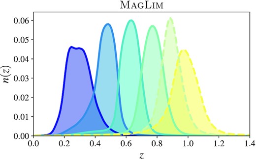
Redshift distributions of the fiducial (solid lines) and non-fiducial (broken lines) galaxy samples used in this study. The distributions are normalized so that their integral is 1. Details about the calibration of these distributions can be found in Cawthon et al. (2022).
Redshift slices and number of galaxies used in this study for the maglim sample.
| maglim | |
|---|---|
| Redshift bin | Ngal |
| 0.20 < z < 0.40 | 2236462 |
| 0.40 < z < 0.55 | 1599487 |
| 0.55 < z < 0.70 | 1627408 |
| 0.70 < z < 0.85 | 2175171 |
| 0.85 < z < 0.95 | 1583679 |
| 0.95 < z < 1.05 | 1494243 |
| maglim | |
|---|---|
| Redshift bin | Ngal |
| 0.20 < z < 0.40 | 2236462 |
| 0.40 < z < 0.55 | 1599487 |
| 0.55 < z < 0.70 | 1627408 |
| 0.70 < z < 0.85 | 2175171 |
| 0.85 < z < 0.95 | 1583679 |
| 0.95 < z < 1.05 | 1494243 |
3.2 y-maps
As mentioned previously, the tSZ effect is typically measured in terms of the Compton-y parameter. Typically, y-maps are built using a linear combination of individual frequency mm-wave/microwave maps (see Delabrouille & Cardoso 2009, for a review) and contain valuable cosmological information (Komatsu & Seljak 2002, and references therein). In this work however, we focus on the cross-correlation between y and the galaxy counts. The southernmost part of the footprint of DES was designed to overlap with the South Pole Telescope’s SPT-SZ survey area (Story et al. 2013). However, there is a significant fraction of the DES Y3 footprint that does not overlap with the SPT-SZ survey. Therefore, we use the SPT-SZ + Planck maps for Dec <−40 deg and the Planck MILCA y-map (Planck Collaboration XIII 2016a) for Dec >−39 deg (which we will refer to as MILCA hereafter). Both of the y-maps that we use in our analysis are shown in Fig. 2. We provide additional details about the maps we use in the following subsections.
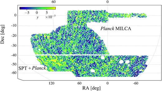
Combined SPT + Planck y-map in equatorial coordinates displayed using an equal-area McBryde-Thomas flat-polar quartic projection. The southern region (Dec < −40 deg.) corresponds to the SPT + Planck minimum variance y-map from Bleem et al. (2022), and the northern region (Dec > −39 deg.) corresponds to the MILCA y-map from Planck Collaboration XIII (2016a). We choose to have a gap between the two regions in order to improve the level of independence of our results. We transform the original data products to healpix resolution Nside = 2048. For display purposes, the maps shown have been smoothed with a Gaussian (FWHM = 0.25 deg) beam.
3.2.1 SPT-SZ + Planck y-maps from Bleem et al. (2022)
For this work, we focus on the component-separated y-maps using a combination of data from the SPT-SZ survey and Planck (Bleem et al. 2022) which are publicly available.3 The maps cover ∼2500 deg2 of the southern sky (with ∼1800 deg2 overlapping with DES Y3 galaxies) with a 1.25 arcmin resolution. In this work, we use the minimum variance y-map presented in Bleem et al. (2022) for our fiducial measurements because it has the lowest noise and the smallest beam size. Additionally, we use the CMB–CIB-nulled y-map to test the presence of CIB contamination in our measurements. For details about these maps, the algorithms behind their construction, and their validation, we refer the readers to Bleem et al. (2022).
In addition to the publicly available maps, we test a custom CIB-reduced (which we will refer to as CIB-nulled) map to ensure a low-level of CIB contamination. This map is generated using the same y-map implementation presented in Bleem et al. (2022). The main difference between the CMB–CIB-nulled (or ‘three-component’) map from Bleem et al. (2022) and our CIB-nulled map (which would be a ‘two-component’ map), is that for the latter we focus on minimizing the residual CIB using the CIB model presented in Reichardt et al. (2021), whereas the CMB-CIB-nulled map not only tries to minimize the CIB residual but also the CMB (which should not correlate with DES galaxies). This results in the CMB–CIB-nulled map having a higher noise level.
3.2.2 MILCA y-map from Planck Collaboration XIII (2016a)
We follow previous analyses (Planck Collaboration XIII 2016a; Hurier & Lacasa 2017; Pandey et al. 2019; Koukoufilippas et al. 2020) and use the MILCA y-map from the Planck collaboration (Planck Collaboration XIII 2016a). This map4 has a beam size of FWHM = 10 arcmin. We apply the 40 per cent Galactic mask and point source mask presented in Planck Collaboration XIII (2016a). The MILCA y-map is generated by combining different frequency maps from the Planck mission. This reconstruction method allows the introduction of external templates to remove unwanted components, such as the CIB. However, the minimization of the CIB signal depends on the particular templates used, and, as the CIB-induced bias decreases, the noise level increases. Moreover, as the CIB maps are not totally correlated across frequencies, its contribution cannot be fully removed (Hurier, Macías-Pérez & Hildebrandt 2013). Therefore, although the MILCA y-map uses CIB templates to minimize the CIB contamination, the effect of any residual CIB leakage on the cross-correlation with galaxies or shear should still be considered carefully.
4 ANALYSIS
In this section, we describe the different components of the analysis. In Section 4.1 we describe how we construct the data vector; in Section 4.2 we describe the covariance matrix we use; in Section 4.3 we describe our choice of scale cuts; in Section 4.4 we introduce our inference framework; in Section 4.5 we perform a series of diagnostic tests on our measurements to ensure there is no significant systematic contamination.
4.1 Measurement
Using the galaxy samples and y-maps described in the previous sections as input, we measure the power spectrum using the pseudo-CℓMASTER algorithm (Hivon et al. 2002) as implemented in NaMaster (Alonso et al. 2019). To do this, we first construct a galaxy density map from the galaxy catalogue by filling each pixel of the map by |$\delta _{g}=\frac{n_{g} - \bar{n}_{g}}{\bar{n}_{g}}$|, where ng is the number of galaxies in each pixel and |$\bar{n}_{g}$| is the mean galaxy number count per pixel. This is done for each of the tomographic bins and the map is constructed with a healpix format of Nside = 2048. The y-maps are downgraded to Nside = 2048 to match the galaxy density maps. Alongside the galaxy density maps, we generate weight maps by summing the weights of each galaxy within a pixel. The weights here are designed to correct for the effect of systematic effects that are imprinted via different survey properties described in Rodríguez-Monroy et al. (2022).
We use logarithmic binning in ℓ with the following bandpower edges: [150, 195, 254, 332, 433, 564, 736, 959, 1251, 1631, 2126, 2772, 3614, 4712, 6142]. The measured power spectra are shown in Figs 3 and 4 for the southern (using the SPT-SZ + Planck maps) and northern (using the MILCA map) regions, respectively. The grey shaded areas are not considered in our fiducial analysis (see Section 4.3). Comparing Figs 3 and 4, the measured |$C^{\rm gg}_{\ell }$| agree well between the two regions of sky at the scales we consider. This is a good first check to show that the galaxy sample is homogeneous across the sky. For |$C^{\rm gy}_{\ell }$|, while the large-scale measurements are in good agreement, we notice some differences at small scales (ℓ > 500) between the two regions. This is a consequence of the different smoothing scale used in the SPT-SZ + Planck and MILCA y-maps.
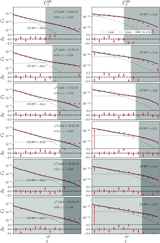
Measured galaxy–galaxy (left-hand column, |$C^{\rm gg}_{\ell }$|) and galaxy-y (right-hand column, |$C_{\ell }^{\rm gy}$|) power spectra and best-fitting HOD (solid black lines) for the southern of the DES footprint using the SPT-SZ + Planck y-map. The lower sub-panels show the residuals divided by the uncertainty, which we denote as Δℓ. The signal-to-noise ratio are annotated for each redshift bin. The |$\chi ^{2}/\rm {ndof}$| values included in the left-hand panels correspond to the total (|$\rm gg + gy)$| χ2.
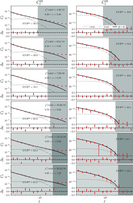
Measured galaxy–galaxy (left-hand column, |$C^{\rm gg}_{\ell }$|) and galaxy-y (right-hand column, |$C_{\ell }^{\rm gy}$|) power spectra and best-fitting HOD (solid black lines) for the northern region of the DES footprint using the MILCA y-map correcting for the CIB contribution (see details in Section 4.5). The lower subpanels show the residuals divided by the uncertainty, which we denote as Δℓ. More details are described in Fig. 3.
In Figs 3 and 4, we also quote the signal-to-noise ratio (SNR), which we calculate as |$\mathrm{SNR}^{uv} = \sqrt{C_{\ell }^{uv} \mathcal {C}_{\ell ,\ell ^{\prime }}^{-1}C_{\ell ^{\prime }}^{uv}}$|, where |$\mathcal {C}_{\ell , \ell ^{\prime }}^{-1}$| is the inverse covariance matrix. We restrict the calculation of the SNR to the scales that are considered in our fiducial analysis ℓ > 150 and k < 0.7 Mpc−1. The choice of these scale-cuts is discussed in Section 4.3.
4.2 Covariance matrix
We use a jackknife (JK) covariance matrix in this analysis in order to appropriately capture any spatial variation in the data beyond the analytical model. We use 75 and 92 roughly equal-area JK patches in the southern and northern regions. The JK patches are generated via the k-means algorithm implementation included in the TreeCorr package (Jarvis, Bernstein & Jain 2004).
The JK-estimated mean data vector is
where X corresponds to Cgg or Cgy here, NJK is the number of JK patches, i indicates individual measurements of X(ℓ) leaving one JK patch i out. The corresponding covariance matrix |$\mathcal {C}$| is given by
We compare our JK estimates with the analytical covariance computed as described in Koukoufilippas et al. (2020), finding agreement within |$20{{\ \rm per\ cent}}$| for all bins (where the JK-estimated covariance is larger).
As the jackknife covariance is known to be noisy and introduces a bias when inverting, we follow Kaufman (1967), Hartlap, Simon & Schneider (2007) and multiply it by a factor H to get the unbiased covariance
where Nband is the number of bandpowers we use.
4.3 Scale cuts
In this work, we explore two regimes of the data vectors separately: the large, linear scales and the small, highly non-linear scales. The fact that we have not been able to coherently model the two regimes under the same model is mainly limited by our ability to model the 1-to-2 halo transition region for |$C_{\ell }^{\rm gg}$|, which has been known to be challenging (Mead et al. 2015; Hadzhiyska et al. 2020). This motivates us first to look separately at the large-scale results, which are more robust to the small-scale modelling uncertainties, and then explore ways to extract information on smaller scales with some assumptions on the HOD. The small-scale analysis also takes advantage of the SPT-SZ + Planck y-maps which are higher resolution than the MILCA y-map, allowing us to probe further into the 1-halo term of |$C_{\ell }^{\rm gy}$|.
For the large-scale analysis, we use scales ℓ < ℓmax, with |$\ell _{\rm max, i} = k_{\rm max} \chi (\bar{z}_{i}) - 1/2$|, with kmax = 0.7 Mpc−1 (which corresponds to ℓmax = 864, 1259, 1636, 1946, 2171, 2320 for redshift bins 0 to 5, respectively), and |$\chi (\bar{z}_{i})$| the comoving distance at the mean redshift of each bin. In addition, we ignore the modes below ℓmin = 150 since our jackknife covariances are not accurate for these modes, given that the typical jackknife region is smaller than the modes that we want to map. For our large-scale analysis, we apply these same cuts to |$C_{\ell }^{\rm gy}$|. The priors associated with the model parameters for the large-scale analysis are listed in Table 2.
| Parameter | Fiducial | Prior |
|---|---|---|
| log10Mmin/M⊙ | – | |$\mathcal {U}(10, 16)$| |
| σlnM | 0.15 | Fixed |
| log10M0/M⊙ | log10Mmin/M⊙ | – |
| |$\log _{10} M^{\prime }_{1}/\mathrm{M}_{\odot }$| | – | |$\mathcal {U}(10, 16)$| |
| αs | – | |$\mathcal {U}(0, 3)$| |
| fc | 1 | Fixed |
| βg | – | |$\mathcal {U}(0.1, 10)$| |
| βmax | – | |$\mathcal {U}(0.1, 10)$| |
| ρgy | – | |$\mathcal {U}(-1, 1)$| |
| bH | – | |$\mathcal {U}(0, 1)$| |
| σz, 0 | 0.975 | |$\mathcal {N}(0.975, 0.062)$| |
| Δz0 | −0.009 | |$\mathcal {N}(-0.009, 0.007)$| |
| σz, 1 | 1.306 | |$\mathcal {N}(1.306, 0.093)$| |
| Δz1 | −0.035 | |$\mathcal {N}(-0.035, 0.01)$| |
| σz, 2 | 0.870 | |$\mathcal {N}(0.870, 0.054)$| |
| Δz2 | −0.005 | |$\mathcal {N}(-0.005, 0.006)$| |
| σz, 3 | 0.918 | |$\mathcal {N}(0.918, 0.051)$| |
| Δz3 | −0.007 | |$\mathcal {N}(-0.007, 0.006)$| |
| σz, 4 | 1.080 | |$\mathcal {N}(1.080, 0.067)$| |
| Δz4 | 0.002 | |$\mathcal {N}(0.002, 0.007)$| |
| σz, 5 | 0.845 | |$\mathcal {N}(0.845, 0.073)$| |
| Δz5 | 0.002 | |$\mathcal {N}(0.002, 0.008)$| |
For the small-scale analysis (see Section 6), we rely on the HOD and bias parameters obtained from the large-scale results, and fit our model to the measured |$C_{\ell }^{gy}$| using the parameters and priors described in Table 3 for the tSZ profile in equation (15). We fix γ = 0.31 as in Arnaud et al. (2010), as we notice that we are insensitive to the value of this parameter. For our analysis in this regime, we restrict our analysis to scales larger than kmax = 2.5 Mpc−1, as we observed that the modelling starts to fail to describe smaller scales. Furthermore, as shown in Rodríguez-Monroy et al. (2022), there is indication that the correction of systematic effects in the galaxy clustering measurement is less effective on the smallest scales. These effects were included at the covariance level for DES Collaboration (2022), Porredon et al. (2022) in real space.
Parameters and priors used in the small-scale analysis. We fix γ to the value found in Arnaud et al. (2010).
| Parameter | Prior |
|---|---|
| α | |$\mathcal {U}(0.3, 4)$| |
| β | |$\mathcal {U}(0.2, 10)$| |
| cP | |$\mathcal {U}(0.1, 5)$| |
| γ | 0.31 |
| Parameter | Prior |
|---|---|
| α | |$\mathcal {U}(0.3, 4)$| |
| β | |$\mathcal {U}(0.2, 10)$| |
| cP | |$\mathcal {U}(0.1, 5)$| |
| γ | 0.31 |
4.4 Likelihood and inference
We assume a Gaussian likelihood for the data vector of measured correlation functions, |$\vec{d}$|, given a model, |$\vec{m}$|, generated using the set of parameters |$\vec{p}$|:
where the sums run over all of the N elements in the data and model vectors. The posterior on the model parameters is then given by:
where |$P_{\rm prior}(\vec{p})$| is a prior on the model parameters.
We sample the posterior by running a Markov Chain Monte Carlo using the ensemble sampler implemented in emcee (Foreman-Mackey et al. 2013).
4.5 Systematics tests
Precision measurements of the galaxy power spectrum |$C_{\ell }^{\rm gg}$| can be affected by observing conditions or the presence of bright objects, which can lead to systematic biases in the measured |$C_{\ell }^{\rm gg}$|. In other studies using these samples (DES Collaboration 2022; Pandey et al. 2022; Porredon et al. 2022; Rodríguez-Monroy et al. 2022), these systematic biases are mitigated by the usage of weights on each galaxy (for details see Rodríguez-Monroy et al. 2022). We follow the same approach and adopt the weights as described in Section 4.1. The galaxy-y cross-correlation |$C_{\ell }^{\rm gy}$|, on the other hand, should be much less affected by the particular observing conditions of the DES galaxies since it is a cross-correlation measurement of two independent data sets. However, |$C_{\ell }^{\rm gy}$| can be affected by other astrophysical systematic effects associated with foregrounds. We test the effect of three of them: dust, bright radio sources, and the CIB.
Dust: We use two sets of independent reddening maps, the maps presented in Delchambre et al. (2022) and the maps presented in Lenz, Hensley & Doré (2017), and compare the power spectra results with and without deprojecting (Elsner, Leistedt & Peiris 2017; Alonso et al. 2019), these maps from the galaxy and y-maps. The idea behind this test is the following: deprojection (or mode projection) essentially assumes that the true signal of interest (in our case |$C^{gy}_{\ell }$|) is not correlated with the foregrounds, and uses a template of the foregrounds to obtain the cleaned, unbiased power spectra. In the case that the foregrounds are correlated with the signal, deprojection can produce overcorrected power spectra. This means, if the difference between the deprojected signal and the non-deprojected signal is not statistically significant, the impact of the foreground in the signal is likely small. We carry out the full analysis with deprojected and non-deprojected galaxy autospectrum and galaxy-y cross spectrum. We find that the maximum absolute value across all redshift bins for the shift of the best fit (1 − bH) is ≈0.23σ, where σ is the statistical uncertainty.
Bright radio sources: Radio sources are a known contaminant of the tSZ maps (Bleem et al. 2022). For this test we focus on the MILCA map, as their masking threshold is substantially larger than the SPT-SZ + Planck maps (∼200 mJy at Planck 143 GHz which goes into MILCA vs ∼6 mJy at 150 GHz for SPT-SZ). We check the effect of these sources by applying an additional mask for sources brighter than 1 mJy in the 1.4 GHz NVSS catalogue (Condon et al. 1998). We find that the maximum absolute value for the shift across all redshift bins of the best fit (1 − bH) is ≈0.15σ when this additional mask is applied.
- CIB: One of the most important contaminants of |$C_{\ell }^{\rm gy}$| is the CIB, as it is correlated with both the galaxy positions and the y-map (Chiang et al. 2020; Koukoufilippas et al. 2020; Gatti et al. 2022). In order to test for the effect of CIB contamination in our measurements we estimate the CIB leakage in |$C_{\ell }^{\rm gy}$|. The idea is the following: The SPT-SZ + Planck y-maps and the MILCA map are constructed using a linear combination of frequency channels. Schematically this can be written as:where yILC denotes the component separated y-map, wt is a vector containing weights (or coefficients) to be multiplied to the individual frequency channels,5 and x(p) is a vector containing the individual frequency channels. In reality, the frequency channel maps contain various foregrounds:(30)$$\begin{eqnarray} y^{\rm ILC}(p)={\bf w}^{t}x(p), \end{eqnarray}$$Since the relationship is linear, we can see that the amount of CIB residuals in our map can be computed using:(31)$$\begin{eqnarray} x(p,\nu)&=&x^{\rm CMB}(p,\nu)+x^{\rm CIB}(p,\nu) \\ &&+x^{\rm tSZ}(p,\nu)+x^{\rm kSZ}(p,\nu)+x^{\rm radio}(p,\nu)+ \ldots \end{eqnarray}$$This implies that we need a clean map of the CIB for every frequency channel that goes into the component separation algorithm. Unfortunately, while we do have relatively clean maps of the CIB at higher frequencies (353/545/857 GHz), such maps do not exist for the lower frequency channels (Planck 100/143/217 or SPT 95/150/220 GHz) since it is challenging to disentangle CIB from other astrophysical components at the those frequencies. Therefore, we make predictions of these maps by taking the 353 GHz map from Lenz, Doré & Lagache (2019), and scaling down the amplitude of that map assuming an SED of the CIB.6(32)$$\begin{eqnarray} y^{\rm CIB}(p)={\bf w}^{t}x^{\rm CIB}(p,\nu). \end{eqnarray}$$
Using this convention, we estimate the CIB residual in the y-maps, yCIB, in each of the maps used in this analysis. We then compute the cross-correlation between each yCIB-maps and our galaxy samples, |$C_{\ell }^{gy,{\rm CIB}}$|, and estimate the ratio between this measurement and the original power spectra. We find that, in the range of scales considered, the median value of this ratio is |$\lt 1{{\ \rm per\ cent}}$| for the minimum variance SPT-SZ + Planck map, as shown in Fig. 5. This is not the case for the MILCA y-map, which show significant levels of CIB contamination for the last three bins considered in our analysis, in line with the results found by Pandey et al. (2019), Gatti et al. (2022).
As a second robustness test, we compare our fiducial measurements using the minimum variance map from Bleem et al. (2022) with the measurements using CIB-CMB-nulled y-map from Bleem et al. (2022). In addition to this map, we also compare with the custom CIB-nulled version of the y-map described in Section 3. In Fig. 6 we show the best-fitting (1 − bH) values for different SPT-SZ + Planck maps. For the MILCA map, we show the results for the original maps, and after correcting for CIB. This correction consists on subtracting the contribution of yCIB described above from the original y-map, i.e, yMILCA-corr = yMILCA − yCIB. We see that the different SPT-SZ + Planck results are compatible with each other, and compatible with the MILCA results after applying the CIB correction. Given the size of the systematic CIB correction using the MILCA map, we choose not to combine the CIB-corrected MILCA (1 − bH) measurements with those obtained from SPT-SZ + Planck in our final results, and only use it as a cross-check here.
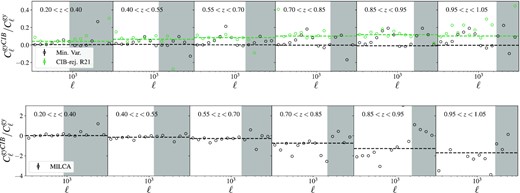
Top panel: Relative CIB leakage in the SPT-SZ + Planck maps, |$C_{\ell }^{gy^{CIB}}/C_{\ell }^{yg}$|. The dashed line represents the median ratio within the considered scale cuts. Bottom panel: CIB leakage for MILCA y-map. For the last 2 redshift bins the CIB signal is dominant.
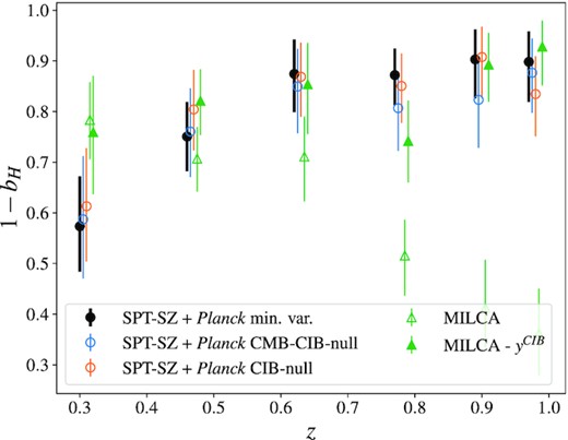
Best-fitting (1 − bH) values as a function of redshift for different maps, showing the impact of CIB on these measurements. Our fiducial values (SPT-SZ + Planck min. var.) are shown as the solid black circles.
5 LARGE-SCALE ANALYSIS: CONSTRAINTS ON HYDROSTATIC MASS BIAS
In this section, we examine the large-scale constraints from the |$C_{\ell }^{\rm gg}+C_{\ell }^{\rm gy}$| measurements. As discussed in Section 1, on these large scales, since |$C_{\ell }^{\rm gg}\propto b_{g}^{2}$|, where bg is the galaxy bias, and |$C_{\ell }^{\rm gy}\propto b_{g} \langle b_{h}P_{e}\rangle$|, the combination helps us constrain the quantity 〈bhPe〉, which is directly related to the hydrostatic mass bias bH.
We use the modelling framework described in Section 2 and the methodology described in Section 4, fitting the large scales with k ≤ 0.7 Mpc−1. In order to make a fair comparison with other studies in the literature, we fix the gas profile parameters to their fiducial values (α, β, γ, cP) = (1.33, 4.13, 0.31, 1.81) (Planck Collaboration XVI 2013). We derive the model fits shown in Figs 3 and 4. The grey dash (dotted-dash) lines show the 1-halo (2-halo) component of the fit and the solid black line shows the full model. In each panel the lower sub-panel shows the residual of the fit divided by the uncertainty. In general, we find good fits to the measurements in all redshift bins, including the last two. The goodness-of-fit and corresponding PTE are shown in Table 4. The good quality of the fits in the last two bins is in agreement with the interpretation put forward by Chang et al. (2023), that there appears to not be significant systematic contamination in the galaxy clustering measurements for these bins. One can also see clearly the |$C_{\ell }^{\rm gg}$| data points deviating from the model at the smallest scales (large ℓ) which we do not use for the fits – there is excess power in the measurements that is not described by a typical 1-halo term. This deviation starts fairly consistently at ℓ ∼ 3000 (corresponding to θ ∼ 3.6 arcmin) across all bins and is consistent with what was found in Rodríguez-Monroy et al. (2022), where the small-scale galaxy clustering could be contaminated by systematic effects (see fig. 6 in that paper).
Summary table with the average redshift, best-fitting chi-square to our fiducial model and number of degrees of freedom, probability to exceed (PTE), the inferred hydrostatic bias and average bias-weighted electron pressure for the different redshift bins of the maglim sample, when cross-correlated with SPT-SZ + Planck and MILCA y-maps. The last two bins are shown in grey as they are not part of our fiducial sample.
| Bin | 〈z〉 | χ2/ndof | PTE | bH | 〈bhPe〉 [meV cm−3] |
|---|---|---|---|---|---|
| SPT-SZ + Planck | |||||
| 0 | 0.30 | 5.46/12 | 0.94 | |$0.43^{+0.09}_{-0.10}$| | |$0.16 ^{+0.03}_{-0.04}$| |
| 1 | 0.46 | 17.27/14 | 0.24 | |$0.25^{+0.07}_{-0.07}$| | |$0.28 ^{+0.04}_{-0.05}$| |
| 2 | 0.62 | 4.72/16 | 1.00 | |$0.13^{+0.08}_{-0.07}$| | |$0.45 ^{+0.06}_{-0.10}$| |
| 3 | 0.77 | 18.37/18 | 0.43 | |$0.13^{+0.06}_{-0.05}$| | |$0.54 ^{+0.08}_{-0.07}$| |
| 4 | 0.89 | 10.58/18 | 0.91 | |$0.10^{+0.08}_{-0.06}$| | |$0.61 ^{+0.08}_{-0.06}$| |
| 5 | 0.97 | 20.04/18 | 0.33 | |$0.10^{+0.08}_{-0.06}$| | |$0.63 ^{+0.07}_{-0.08}$| |
| milca (CIB corrected) | |||||
| 0 | 0.30 | 4.28/12 | 0.99 | |$0.24 ^{+0.12}_{-0.11}$| | |$0.24 ^{+0.09}_{-0.07}$| |
| 1 | 0.46 | 6.01/14 | 0.99 | |$0.19 ^{+0.07}_{-0.06}$| | |$0.32 ^{+0.04}_{-0.06}$| |
| 2 | 0.62 | 7.28/16 | 0.99 | |$0.15 ^{+0.10}_{-0.08}$| | |$0.51 ^{+0.17}_{-0.08}$| |
| 3 | 0.77 | 16.08/18 | 0.62 | |$0.26 ^{+0.08}_{-0.08}$| | |$0.40^{+0.08}_{-0.11}$| |
| 4 | 0.89 | 13.15/18 | 0.86 | |$0.11 ^{+0.07}_{-0.06}$| | |$0.57 ^{+0.07}_{-0.07}$| |
| 5 | 0.97 | 22.55/18 | 0.14 | |$0.07 ^{+0.08}_{-0.05}$| | |$0.65 ^{+0.08}_{-0.10}$| |
| milca (raw) | |||||
| 0 | 0.30 | 3.17/12 | 1.00 | |$0.22 ^{+0.08}_{-0.08}$| | |$0.27 ^{+0.05}_{-0.05}$| |
| 1 | 0.46 | 6.97/14 | 0.99 | |$0.29 ^{+0.06}_{-0.06}$| | |$0.28 ^{+0.04}_{-0.04}$| |
| 2 | 0.62 | 13.13/16 | 0.73 | |$0.29 ^{+0.09}_{-0.08}$| | |$0.37 ^{+0.10}_{-0.07}$| |
| 3 | 0.77 | 15.58/18 | 0.71 | |$0.48 ^{+0.08}_{-0.07}$| | |$0.21^{+0.04}_{-0.04}$| |
| 4 | 0.89 | 20.10/18 | 0.27 | |$0.59 ^{+0.08}_{-0.09}$| | |$0.19 ^{+0.07}_{-0.04}$| |
| 5 | 0.97 | 19.68/18 | 0.35 | |$0.64 ^{+0.08}_{-0.09}$| | |$0.20 ^{+0.07}_{-0.04}$| |
The inferred best-fitting values of bH and average bias-weighted electron pressure 〈bhPe〉 are summarized in Table 4. We plot〈 bhPe〉 as a function of redshift in the left-hand panel of Fig. 7 to compare with a compilation of previous literature (Vikram et al. 2017; Pandey et al. 2019; Chiang et al. 2020; Koukoufilippas et al. 2020; Yan et al. 2021; Chen et al. 2023). The eight solid black points represent our fiducial result, while the four hollowed points are from the highest two maglim redshift bins. Among the previous results plotted in Fig. 7, Vikram et al. (2017), Pandey et al. (2019) are the most similar to this work where a combination of galaxy clustering and galaxy-y cross-correlation are used and the galaxies are of similar halo mass. Overall, our results (both the fiducial sample and the high-redshift bins) appear broadly consistent with previous studies in the literature, and represent the most precise measurements at high redshift (z > 0.8) due to the depth of DES Y3 data.
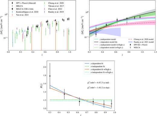
Top left-hand panel: Hydrostatic bias results as a function of redshift and comparison with previous results. Top right-hand panel: Best-fitting redshift-independent model (cyan solid line), and redshift dependent model (black solid line) for the hydrostatic bias. We also show the equivalent best-fitting results when including the last two redshift bins in the fits (broken magenta and green lines). For easy comparison the best-fitting model from Chiang et al. (2020) (red dot-dashed line), and from Pandey et al. (2022) are included (shaded blue region). The model for Pandey et al. (2022) is only included up to z ∼ 0.7, as for higher redshifts, due to the lensing kernel, the shear × y constraining power gets reduced (Pandey private comm.). Bottom panel: Hydrostatic bias expressed as B as a function of redshift, and best-fitting redshift-dependent model (solid lines), and redshift-independent model (broken lines). We also include the results for the two high-redshift bins, and the best-fits including these points.
Next we examine the redshift dependence of 〈bhPe〉. Following Chiang et al. (2020), we fit |$B=\frac{1}{1-b_{H}}$| as a function of redshift with a power-law model and convert the resulting fit to the corresponding model fit in 〈bhPe〉. In particular, we assume the following model
and fit for p0 and p1. Setting p1 = 0 gives the redshift-independent model, which we also examine.
In order to account for the correlation between the data points in different redshift bins, we model the correlation matrix to be proportional to the overlaps in the redshift distributions between redshift bins. This is a reasonable approximation given the uncertainty in 〈bhPe〉 and therefore B is dominated by the large-scale uncertainties in Cgg, whose correlation between redshift bins is directly related to the overlap in the redshift bins. The covariance matrix then becomes:
where rij is the migration matrix given by (Benjamin et al. 2010):
where ni/j(z) is the normalized redshift distribution of the redshift i/j, and zi/j, low, zi/j, hi are the photo-z edges of each bin. This matrix is guaranteed to be invertible by the Gershgorin theorem as long as it is strictly diagonally dominant (Benjamin et al. 2010), i.e.
Essentially, this means that the photo-z distributions for each bin should be dominated by galaxies with their true redshifts within that bin. This is the case when we use the photo-z distributions in Fig. 1.
With this procedure, we fit our data using the model of equation (33). We find that assuming a redshift independent B gives B = 1.22 ± 0.06 with χ2/ndof = 4.47/3, and Bayesian evidence |$\log {\mathcal {Z}}=-1.34 \pm 0.05$|. On the other hand, assuming the same redshift-dependent B model as Chiang et al. (2020), we obtain |$B = 2.10^{+0.61}_{-0.49}\left(1+z\right)^{-1.09^{+0.53}_{-0.53}}$| with χ2/ndof = 1.45/2, |$\log {\mathcal {Z}}=-1.32 \pm 0.04$|. That is, we find a Bayes’ factor of 0.88, indicating no significant preference between these models. We plot both models on the upper right-hand panel of Fig. 7 and compare to model fits in previous work of Chiang et al. (2020) and Pandey et al. (2022) in the bottom panel. We also show the fits including the two high-redshift bins. In general, we find that our overall constraining power on the model is at a similar level as Chiang et al. (2020), but we prefer a decreasing trend in the values of B as a function of redshift, instead of an increasing trend. This might be related to our larger values of 〈bhPe〉 at z > 0.7 compared to those found by Chiang et al. (2020) as seen in the upper left-hand panel of Fig. 7. Our findings for p1 are in line with the results in Wicker et al. (2022), which find |$p_{1} = -1.14 ^{+0.33}_{-0.73}$| for low mass, low redshift clusters |$(z \lt 0.2, M \lt 5.89 \times 10^{14} \, \mathrm{M}_{\odot })$|. This decreasing trend of B as a function of redshift has also been found in the literature in cluster studies (von der Linden et al. 2014; Hoekstra et al. 2015; Smith et al. 2016; Sereno & Ettori 2017; Eckert et al. 2019). We also find that when including the two highest redshift bins, the fit does not change significantly, suggesting that even for the slightly poorer model fit in these bins and potential systematic contamination, the results using them are actually consistent with only using the fiducial sample.
Both the effect of the halo mass evolution as well as changes in the gas profiles can result in different measurements of 1 − bH at various redshifts. We argue that the evolution in halo mass of our particular galaxy sample does not fully explain the evolution in the halo mass since the constraints on the HOD model through |$C_{\ell }^{\rm gg}$| measurements suggest that the halo mass of our sample does not significantly evolve with redshift (see Appendix A), which is consistent with the results of Zacharegkas et al. (2022), implying that the redshift evolution of 1 − bH can be primarily attributed to the evolution of gas characteristics.
Using the best-fitting GNFW parameters and value for 1 − bH, we estimate the amplitude of |$\tilde{Y}_{500}$| of the haloes that contribute the most to the first redshift bin and compare the result with those from Lim et al. (2018), who studied the gas profiles around galaxy groups in the redshift range 0 < z < 0.2. The results are shown in Fig. 8. We recover values compatible with those measured by Lim et al. (2018).
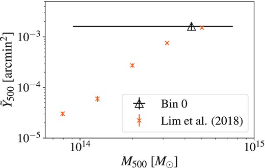
Reconstructed Y − M relation using our fiducial GNFW parameters, and our large-scale hydrostatic bias results. We show the mean inferred |$\tilde{Y}_{500}$| at the mean predicted halo mass for our first redshift bin (black open triangle). The horizontal error bar is estimated from the 16th and 84th percentiles of mass contributing to the signal, and the vertical error bar comes from the 16th and 84th percentiles of the inferred |$\tilde{Y}_{500}$| models. We compare with the measurements using galaxy groups from Lim et al. (2018) (orange crosses).
The comparison with Pandey et al. (2022) shows good agreement at low redshift, but there is an apparent tension at z > 0.6. The authors in Pandey et al. (2022) point to a lack of sensitivity to low-mass haloes that contribute to the overall signal as a possible source for the tension between their work and other constraints from galaxy-y cross-correlation. Moreover, due to the lensing kernel the shear-y cross-correlations, the constraining power gets reduced at higher redshifts (Pandey private comm.). Future shear-y cross-correlation studies using SPT data will help clarify the origin of this tension (Omori et al., in preparation).
6 SMALL-SCALE ANALYSIS: CONSTRAINTS ON GAS PROFILES
We now turn our attention to the small-scale information in the galaxy-y cross-correlation. As discussed in Section 4.3, this takes advantage of the high-resolution and low-noise nature of the SPT-SZ + Planck y-map. We also discussed in Section 4.3 that there are uncertainties in both the modelling and measurements of |$C_{\ell }^{\rm gg}$|. Thus, to extract the small-scale information in the gas profiles in |$C_{\ell }^{\rm gy}$|, we make a couple of assumptions and adjustments to the analysis. In essence, we fix the HOD constraints using the large scales as in Section 5 and Appendix A. Then, we fit the |$C_{\ell }^{\rm gy}$| with kmax = 2.5 Mpc−1, freeing the GNFW gas profile parameters (α, β, γ).
In order to get some physical intuition about our small-scale results, we compare our |$C_{\ell }^{gy}$| measurements up to kmax = 2.5 Mpc−1 with the GNFW model parameters for the cosmo-OWLS suite (Le Brun et al. 2014) reported in Le Brun et al. (2015) for the ‘REF’, ‘AGN 8.0’,7 and ‘AGN 8.5’ simulations. Cosmo-OWLS is a set of hydrodynamical simulations and is part of the OverWhelmingly Large Simulations (OWLS; Schaye et al. 2010) project. It has been designed to help improve our understanding of cluster astrophysics and non-linear structure formation by systematically varying several sub-grid physics models, including feedback from supernovae and AGN. One important note is that the best-fitting model in Le Brun et al. (2015) modifies the profiles described by equation (15) by including a mass-dependent concentration, |$c_{P}=c_{P,0}\left(\frac{M}{10^{14} \, \mathrm{M}_{\odot }}\right)^{\delta }$|, and normalization, |$P_{0}=P_{0,0}\left(\frac{M}{10^{14}\, \mathrm{M}_{\odot }}\right)^{\epsilon }$|. The values for the parameters that we use to compare with these simulations are shown in Table 5.
Best-fitting GNFW parameters from Le Brun et al. (2015) for different simulations of the cosmo-OWLS suite.
| Simulation | P0, 0 | α | β | γ | cP, 0 | δ | ϵ |
|---|---|---|---|---|---|---|---|
| REF | 0.528 | 2.208 | 3.632 | 1.486 | 1.192 | 0.051 | 0.210 |
| AGN 8.0 | 0.581 | 2.017 | 3.835 | 1.076 | 1.035 | 0.273 | 0.819 |
| AGN 8.5 | 0.214 | 1.868 | 4.117 | 1.063 | 0.682 | 0.245 | 0.839 |
| Simulation | P0, 0 | α | β | γ | cP, 0 | δ | ϵ |
|---|---|---|---|---|---|---|---|
| REF | 0.528 | 2.208 | 3.632 | 1.486 | 1.192 | 0.051 | 0.210 |
| AGN 8.0 | 0.581 | 2.017 | 3.835 | 1.076 | 1.035 | 0.273 | 0.819 |
| AGN 8.5 | 0.214 | 1.868 | 4.117 | 1.063 | 0.682 | 0.245 | 0.839 |
The best-fitting models are shown in Fig. 9 in black and listed in Table 6. In Fig. 9 we also overlay the prediction of the small-scale |$C_{\ell }^{\rm gy}$| from different hydrodynamical simulations as listed in Table 5. Overall, we find that for the individual redshift bins, and for the scales considered, our model provides a good description of the data and the predictions from simulations broadly follow the same trends and shape of the data vectors
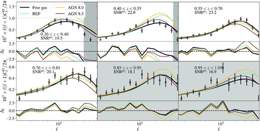
Top panels: Measured power spectra (black circles) and best-fitting GNFW profile (black). We also include the GNFW profiles from Le Brun et al. (2015) for the REF (cyan), AGN 8.0 (orange), and AGN 8.5 (maroon) simulations of the cosmo-OWLS suite. Bottom panels: Residuals relative to the uncertainty, Δℓ for our best-fitting GNFW profile (black line), for the REF model (cyan), for the AGN 8.0 model (orange), and for the AGN 8.5 model (maroon).
Summary of the number of data points, the best-fitting parameters, and the χ2 values against predictions from different simulations for the small-scale measurements in the SPT region described in Section 6. The last two bins are shown in grey as they are not part of our fiducial sample.
| Bin | ndata | α | β | cP | χ2 (free gas) | χ2 (REF) | χ2 (AGN 8.0) | χ2 (AGN 8.5) |
|---|---|---|---|---|---|---|---|---|
| 0 | 11 | |$0.74^{+0.33}_{-0.13}$| | |$5.67^{+2.23}_{-1.81}$| | |$0.58^{+1.17}_{-0.38}$| | 9.7 | 13.6 | 26.6 | 10.5 |
| 1 | 13 | |$0.62^{+0.14}_{-0.08}$| | |$5.89^{+1.61}_{-1.38}$| | |$0.38^{+0.55}_{-0.22}$| | 22.5 | 62.0 | 76.8 | 23.2 |
| 2 | 14 | |$1.78^{+1.30}_{-0.70}$| | |$3.73^{+1.25}_{-0.43}$| | |$2.38^{+0.67}_{-1.18}$| | 6.1 | 6.7 | 6.3 | 15.9 |
| 3 | 14 | |$2.01^{+1.25}_{-0.81}$| | |$4.03^{+1.26}_{-0.53}$| | |$2.24^{+0.60}_{-0.97}$| | 11.3 | 14.1 | 14.8 | 19.8 |
| 4 | 14 | |$1.80^{+1.44}_{-0.92}$| | |$3.06^{+0.75}_{-0.28}$| | |$3.36^{+0.78}_{-1.75}$| | 19.2 | 29.4 | 25.8 | 23.0 |
| 5 | 14 | |$1.38^{+1.50}_{-0.62}$| | |$3.16^{+0.94}_{-0.34}$| | |$3.16^{+1.10}_{-1.87}$| | 21.5 | 26.4 | 34.3 | 20.1 |
In order to quantify the overall agreement between the different models and our measurements, we combine the χ2 in the different redshift bins to a total goodness-of-fit metric
where rij is the migration matrix defined in equation (35). Note that this is equivalent to considering that the only correlations between bins are due to the photometric redshift overlap, and not due to the LSS. Given our scale cuts (ℓ > 150) and the redshift bin width, this is a safe assumption.
We find that the GNFW model with the free gas parameters is the best description of our data with |$\chi ^{2}_{\rm total}/\rm {ndof} = 42/40$| (PTE: 0.37), followed by the AGN 8.5 model |$\chi ^{2}_{\rm total} /\rm {ndof} = 58/52$| (PTE: 0.25).8 The REF simulation is a reasonable but somewhat worse fit with |$\chi ^{2}_{\rm total}/\rm {ndof} = 84/52$| (PTE: 0.003) – we note that we generally expect REF to perform worse than the AGN models as it does not contain any AGN feedback, which is not realistic, as we expect AGN feedback to be very relevant for the observables considered here. Finally, the AGN 8.0 model seems to poorly describe bins 0, and 1, where the latter has a |$\chi ^{2}/\rm {ndof} = 76.8/13$|. The total |$\chi ^{2}_{\rm total}/\rm {ndof} = 108/52$| (PTE:6 × 10⁻⁶) indicates that this model does not describe the data well. We also check whether our model provides a good description of the 1-halo term of |$C_{\ell }^{gy}$|. We do this by computing the chi-square of the best-fitting GNFW model with free parameters restricted to the following range of scales: 0.5 Mpc−1 < k < 2.5 Mpc−1. We obtain |$\chi ^{2}/\rm {ndof} = (3.63/6, 6.38/6, 2.75/6, 1.01/6, 2.64/5, 4.52/6)$|, in each bin respectively, indicating that our model can accurately describe our measurements within the 1-halo regime given our uncertainties.
Taken at face value, the data prefers the AGN 8.5 model over the AGN 8.0 model, indicating that stronger feedback (higher TAGN) is preferred. This is opposite from what is found in Tröster et al. (2021) using cosmic shear only. However, our results do agree with several other previous work including Gatti et al. (2022), Lim et al. (2018), and Tröster et al. (2022). It is worth noting that there are some results in the literature that use the BAHAMAS (McCarthy et al. 2017) simulations model, and the value for best-fitting AGN heating temperature found using this model is different than using the cosmo-OWLS model as is done here. For example, the authors in McCarthy et al. (2017) point out that cosmo-OWLS AGN 8.0 matches best with AGN 7.8 for BAHAMAS.
Our results also seem to indicate that, at low redshifts, the AGN feedback is stronger than at higher redshifts (both AGN 8.0 and AGN 8.5 lines are systematically above the data points in bin 0 and 1, and similar or below the data points in bin 2 and 3), pointing to potential redshift-dependent AGN feedback amplitudes that are somewhat different compared to the cosmo-OWLS simulations. Furthermore, for the first two redshift bins, our GNFW fits prefer smaller values for α, cP and larger values for β than those found for galaxy clusters in Arnaud et al. (2010) and Planck Collaboration XVI (2013), which means that the gas profiles for our galaxy sample are more peaked than typical cluster profiles. We show the ratio of the best-fitting pressure profile to the AGN 8.5 profile at |$M=10^{14}\, \mathrm{M}_{\odot }\, h^{-1}$| in Fig. 10. It is clear from this plot that, in general, the data prefer a profile with higher pressure at small scales r < r500c compared to the AGN 8.5 profile. In addition, there is a clear redshift evolution – this difference is most apparent at high redshift. We also include the best-fitting profile from Planck galaxy clusters, which shows a similar trend as our results and interestingly matches well our results from Bin 2.
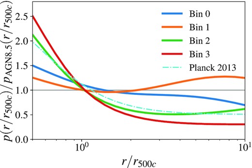
Ratio of the best-fitting gas profiles from the four tomographic bins in our work (solid lines) to the ‘AGN 8.5’ simulation in Le Brun et al. (2015). We also plot best-fitting profile to Planck clusters (dot dashed cyan).
We note that given the small number of simulations we are able to compare to and the uncertainties in the data, we cannot make more generic astrophysical constraints on, e.g. the AGN heating temperature. We can, however, conclude that in the cosmo-OWLS simulation suite, the AGN 8.5 case, with all parameter settings adopted by that simulation, can describe our data within the measurement uncertainties. This will suggest that in future analyses when a plausible small-scale model is needed for, e.g. the matter power spectrum, AGN 8.5 will be a good option. We leave it for future work to apply the methodology of this work to more recent simulation suits that systematically span a larger grid of different baryonic physics such as the Cosmology and Astrophysics with Machine-learning Simulations project (CAMELS; Villaescusa-Navarro et al. 2021).
7 CONCLUSIONS
In this paper, we measure and model the auto and cross-power spectra of galaxy density and the thermal Sunyaev-Zeldovich (tSZ) effect. We use the maglim galaxies from the first 3 yr of DES data and the MILCA y-map, as well the y-map constructed using frequency combinations from SPT-SZ and Planck. There are two main goals of this paper: First we use the large-scale information to constrain the hydrostatic mass bias and compare with previous studies. Secondly, fixing the HOD from the large-scale galaxy density auto- correlation, we fit the galaxy density-y cross-correlation and extract information about the small-scale gas profile. We then compare our results with hydrodynamical simulations.
The main advances of this work are the high density of the maglim sample, which allows us to have a good SNR from redshift 0.2 to 1.0, and the new y-maps from SPT, which probe smaller scales than previous works. Additionally, having three different versions of the SPT y-maps (minimum variance, CMB-CIB-nulled, and CIB-nulled) allows us a better understanding of the main foreground at z > 0.7, the contribution from the CIB.
We model the power spectra using an HOD approach, finding good agreement with previous results (Zacharegkas et al. 2022). We find that our measurements of the hydrostatic bias, bH, are in good agreement with the literature (Vikram et al. 2017; Pandey et al. 2019; Chiang et al. 2020; Koukoufilippas et al. 2020; Yan et al. 2021; Chen et al. 2023).
We measure the evolution of bH with redshift, and find a slight preference for a redshift dependent bH, and find the evolution to be somewhat stronger than previous results. Additional measurements at higher and lower redshifts should be used to pin down the evolution in future work. Our results using the Planck MILCA maps for z ≳ 0.8 show CIB contamination levels of 70 per cent in the measured bH. As a result, these maps should be used with caution for cross-correlation studies. We find that the bias due to the presence of CIB in the MILCA y-map can be mitigated by estimating the contamination term (by propagating external estimated of the CIB at various frequencies through the MILCA weights), and subtracting that contribution from the measured correlation.
Finally, we take advantage of the high-resolution nature of the SPT maps and fit the measured gas profiles to a GNFW profile, and compare with standard profiles from the cosmo-OWLS suite (Le Brun et al. 2015). We find that, overall, our results seem to prefer the strongest of the considered AGN feedback models, AGN 8.5. This agrees with previous results using shear-y cross-correlations (Gatti et al. 2022; Tröster et al. 2022). We also notice that this preference for higher-than-typical AGN feedback is lowered when going to higher redshifts, which may indicate a redshift evolution.
Upcoming data from Advanced ACTPol (Henderson et al. 2016) and SPT-3G (Benson et al. 2014), in combination with the final DES data set and the Hyper Suprime-Cam Subaru Strategic Program (HSC-SSP Aihara et al. 2018) can help us further study this potential evolution, and improve the modelling of the small scales, which constitute one of the main limiting factors of current large-scale structure cosmology analyses.
ACKNOWLEDGEMENTS
The authors would like to acknolwedge the anonymous referee for their comments that helped improve the overall quality of this work. JS thanks Yi-Kuan Chiang for providing 〈bhPe〉 data for comparisons. JS thanks David Alonso for help and feedback throughout the project. We thank the creators of CCL, astropy, numpy, matplotlib, yxg, healpy, HEALPix.
YO and CC are supported by DOE grant DE-SC0021949.
The South Pole Telescope program is supported by the National Science Foundation (NSF) through the grant OPP-1852617 and OPP-2147371. Partial support is also provided by the Kavli Institute of Cosmological Physics at the University of Chicago. Argonne National Laboratory’s work was supported by the U.S. Department of Energy, Office of Science, Office of High Energy Physics, under contract DE-AC02-06CH11357. Work at Fermi National Accelerator Laboratory, a DOE-OS, HEP User Facility managed by the Fermi Research Alliance, LLC, was supported under Contract No. DE-AC02- 07CH11359. The Melbourne authors acknowledge support from the Australian Research Council’s Discovery Projects scheme (DP200101068). The McGill authors acknowledge funding from the Natural Sciences and Engineering Research Council of Canada, Canadian Institute for Advanced research, and the Fonds de recherche du Québec Nature et technologies. The CU Boulder group acknowledges support from NSF AST-0956135. The Munich group acknowledges the support by the ORIGINS Cluster (funded by the Deutsche Forschungsgemeinschaft (DFG, German Research Foundation) under Germany’s Excellence Strategy - EXC-2094 - 390783311), the MaxPlanck-Gesellschaft Faculty Fellowship Program, and the Ludwig-Maximilians-Universität München.
Funding for the DES Projects has been provided by the U.S. Department of Energy, the U.S. National Science Foundation, the Ministry of Science and Education of Spain, the Science and Technology Facilities Council of the United Kingdom, the Higher Education Funding Council for England, the National Center for Supercomputing Applications at the University of Illinois at Urbana-Champaign, the Kavli Institute of Cosmological Physics at the University of Chicago, the Center for Cosmology and Astro-Particle Physics at the Ohio State University, the Mitchell Institute for Fundamental Physics and Astronomy at Texas A&M University, Financiadora de Estudos e Projetos, Fundação Carlos Chagas Filho de Amparo à Pesquisa do Estado do Rio de Janeiro, Conselho Nacional de Desenvolvimento Científico e Tecnológico and the Ministério da Ciência, Tecnologia e Inovação, the Deutsche Forschungsgemeinschaft and the Collaborating Institutions in the Dark Energy Survey.
The Collaborating Institutions are Argonne National Laboratory, the University of California at Santa Cruz, the University of Cambridge, Centro de Investigaciones Energéticas, Medioambientales y Tecnológicas-Madrid, the University of Chicago, University College London, the DES-Brazil Consortium, the University of Edinburgh, the Eidgenössische Technische Hochschule (ETH) Zürich, Fermi National Accelerator Laboratory, the University of Illinois at Urbana-Champaign, the Institut de Ciències de l’Espai (IEEC/CSIC), the Institut de Física d’Altes Energies, Lawrence Berkeley National Laboratory, the Ludwig-Maximilians Universität München and the associated Excellence Cluster Universe, the University of Michigan, NFS’s NOIRLab, the University of Nottingham, The Ohio State University, the University of Pennsylvania, the University of Portsmouth, SLAC National Accelerator Laboratory, Stanford University, the University of Sussex, Texas A&M University, and the OzDES Membership Consortium.
Based in part on observations at Cerro Tololo Inter-American Observatory at NSF’s NOIRLab (NOIRLab Prop. ID 2012B-0001; PI: J. Frieman), which is managed by the Association of Universities for Research in Astronomy (AURA) under a cooperative agreement with the National Science Foundation.
The DES data management system is supported by the National Science Foundation under Grant Numbers AST-1138766 and AST-1536171. The DES participants from Spanish institutions are partially supported by MICINN under grants ESP2017-89838, PGC2018-094773, PGC2018-102021, SEV-2016-0588, SEV-2016-0597, and MDM-2015-0509, some of which include ERDF funds from the European Union. IFAE is partially funded by the CERCA program of the Generalitat de Catalunya. Research leading to these results has received funding from the European Research Council under the European Union’s Seventh Framework Program (FP7/2007-2013) including ERC grant agreements 240672, 291329, and 306478. We acknowledge support from the Brazilian Instituto Nacional de Ciência e Tecnologia (INCT) do e-Universo (CNPq grant 465376/2014-2).
This manuscript has been authored by Fermi Research Alliance, LLC under Contract No. DE-AC02-07CH11359 with the U.S. Department of Energy, Office of Science, Office of High Energy Physics.
We gratefully acknowledge the computing resources provided on Crossover, a high-performance computing cluster operated by the Laboratory Computing Resource Center at Argonne National Laboratory.
This research used resources of the National Energy Research Scientific Computing Center (NERSC), a U.S. Department of Energy Office of Science User Facility located at Lawrence Berkeley National Laboratory, operated under Contract No. DE-AC02-05CH11231.
DATA AVAILABILITY
All DES Year 3 cosmology catalogues are available at https://des.ncsa.illinois.edu/releases/y3a2. This work uses publicly available SPT-SZ + Planck maps at https://pole.uchicago.edu/public/data/sptsz_ymap/ and the Planck MILCA map at https://irsa.ipac.caltech.edu/data/Planck/release_2/all-sky-maps/ysz_index.html. In addition we use the publicly available CIB maps from https://lambda.gsfc.nasa.gov/product/planck/curr/planck_tp_lenz_get.html
Footnotes
bh refers to the halo bias, which is used in the calculation of 〈bhPe〉 as shown in equation (18).
The maps and masks used are publicly available at https://irsa.ipac.caltech.edu/data/Planck/release_2/all-sky-maps/ysz_index.html.
The weights for the SPT map can be found at https://pole.uchicago.edu/public/data/sptsz_ymap/component_map_weights/, while the weights for the MILCA map can be found at https://wiki.cosmos.esa.int/planck-legacy-archive/images/8/83/Milca_nilc_IDL_routines.zip. The MILCA weights used here are also spatially varying and therefore wt is a function of direction.
For this, we use the best-fitting CIB power spectra templates from Reichardt et al. (2021) (and also extrapolations to 353 GHz). We compute the mean amplitude of the CIB model in the ℓ range 100 < ℓ < 1500 for all the frequency channels, and take the scaling factors as the ratio between those values and the value for 353 GHz.
The numbers represent the AGN heating temperatures in the form of log10(TAGN/K) in this naming convention.
We find that for some of the bins, the model using the parameters from the AGN 8.5 simulation have a lower χ2 than our model. This is due to added flexibility in the model by adding a mass dependence in P0 and cP.
References
APPENDIX: HOD CONSTRAINTS FROM GALAXY CLUSTERING
As a by-product of this analysis, we obtain the HOD constraints from galaxy clustering for the DES Y3 MagLim sample. A dedicated HOD analysis of the same sample using a galaxy–galaxy lensing approach was presented in Zacharegkas et al. (2022). Being a cross-correlation, galaxy–galaxy lensing is somewhat less prone to systematic effects. As a result checking the HOD constraints from our analysis using galaxy clustering with Zacharegkas et al. (2022) provides a good test for the robustness of the constraints. In particular, a good test is to compare the galaxy bias obtained using the best-fitting halo model parameters from this work, with the galaxy bias results measured in Zacharegkas et al. (2022). We also compare these bias results with the results obtained in the 3 × 2-point DES Y3 analysis (DES Collaboration 2022) (DES Y3 KP), and the model in Nicola et al. (2020):
With b1 = −0.0624 ± 0.0070, b0 = 0.8346 ± 0.161, α = −1.30 ± 0.19, and D+(z) the linear growth factor at redshift z. In our case we use mlim = 4z + 18. Since our measurements of |$C_{\ell }^{gg}$| are only sensitive to the bgσ8 combination, we decide to compare on these terms instead of the raw galaxy bias, as some of these analyses use slightly different values for σ8. In Fig. A1 we see that all of the results using the DES Y3 are in good agreement. We also see that the results from the SPT and Planck regions agree with each other. Finally, we see that our measurements are compatible with the model from Nicola et al. (2020), despite using a different galaxy sample (DES Y3 versus HSC). We include the best-fitting HOD parameters in Table A1 for reference.

Best-fitting HOD parameters for the SPT and Planck regions.
| Bin | log10Mmin/M⊙ | |$\log _{10}M^{\prime }_{1}/\mathrm{M}_{\odot }$| | αs | βg | βmax | ρgy | Δzi | σz, i |
|---|---|---|---|---|---|---|---|---|
| SPT | ||||||||
| 0 | |$12.1^{+0.3}_{-0.4}$| | |$13.2^{+0.5}_{-1.0}$| | |$0.97^{+0.27}_{-0.22}$| | |$1.0^{+0.2}_{-0.5}$| | |$2.3^{+2.0}_{-0.8}$| | |$0.21^{+0.50}_{-0.40}$| | |$\left(-9.0 ^{+7.7}_{-7.1}\right)\times 10^{-3}$| | |$0.97^{+0.06}_{-0.06}$| |
| 1 | |$12.1^{+0.3}_{-0.3}$| | |$13.1^{+0.8}_{-1.3}$| | |$0.62^{+0.19}_{-0.29}$| | |$1.3^{+0.2}_{-0.1}$| | |$0.9^{+1.1}_{-0.5}$| | |$-0.28^{+0.65}_{-0.25}$| | |$\left(-3.4 ^{+1.2}_{-1.1}\right)\times 10^{-2}$| | |$1.31^{+0.09}_{-0.10}$| |
| 2 | |$12.1^{+0.3}_{-0.3}$| | |$12.9^{+0.6}_{-1.2}$| | |$0.71^{+0.32}_{-0.35}$| | |$1.2^{+0.1}_{-0.1}$| | |$1.9^{+2.6}_{-1.1}$| | |$-0.30^{+0.65}_{-0.28}$| | |$\left(-4.3 ^{+5.9}_{-6.6}\right)\times 10^{-3}$| | |$0.88^{+0.05}_{-0.05}$| |
| 3 | |$12.1^{+0.2}_{-0.2}$| | |$12.7^{+0.6}_{-1.1}$| | |$0.54^{+0.52}_{-0.31}$| | |$1.1^{+0.2}_{-0.3}$| | |$4.0^{+3.6}_{-2.3}$| | |$-0.28^{+0.59}_{-0.41}$| | |$\left(-6.5 ^{+6.1}_{-6.3}\right)\times 10^{-3}$| | |$0.92^{+0.05}_{-0.05}$| |
| 4 | |$12.2^{+0.2}_{-0.2}$| | |$12.6^{+0.7}_{-1.1}$| | |$0.57^{+0.49}_{-0.38}$| | |$1.1^{+0.2}_{-0.4}$| | |$4.7^{+3.6}_{-2.3}$| | |$-0.51^{+0.56}_{-0.26}$| | |$\left(1.4 ^{+7.7}_{-7.2}\right)\times 10^{-3}$| | |$1.08^{+0.07}_{-0.07}$| |
| 5 | |$12.0^{+0.2}_{-0.4}$| | |$12.4^{+0.6}_{-1.0}$| | |$1.06^{+0.32}_{-0.43}$| | |$0.9^{+0.4}_{-0.5}$| | |$5.8^{+3.0}_{-2.2}$| | |$-0.62^{+0.26}_{-0.14}$| | |$\left(2.2 ^{+8.6}_{-8.1}\right)\times 10^{-3}$| | |$0.85^{+0.08}_{-0.07}$| |
| Planck (CIB corrected) | ||||||||
| 0 | |$12.1^{+0.3}_{-0.3}$| | |$12.8^{+0.7}_{-1.3}$| | |$0.68^{+0.33}_{-0.36}$| | |$1.2^{+0.2}_{-0.4}$| | |$3.9^{+4.1}_{-1.9}$| | |$-0.46^{+0.67}_{-0.30}$| | |$\left(-9.2 ^{+7.4}_{-7.2}\right)\times 10^{-3}$| | |$0.98^{+0.06}_{-0.06}$| |
| 1 | |$12.2^{+0.3}_{-0.3}$| | |$13.0^{+0.8}_{-1.5}$| | |$0.61^{+0.32}_{-0.40}$| | |$1.3^{+0.2}_{-0.1}$| | |$1.8^{+3.0}_{-1.0}$| | |$-0.59^{+0.52}_{-0.18}$| | |$\left(-3.4 ^{+1.2}_{-1.2}\right)\times 10^{-2}$| | |$1.31^{+0.10}_{-0.10}$| |
| 2 | |$11.9^{+0.3}_{-0.5}$| | |$13.0^{+0.6}_{-1.2}$| | |$0.84^{+0.18}_{-0.26}$| | |$1.2^{+0.1}_{-0.1}$| | |$0.6^{+0.6}_{-0.3}$| | |$-0.65^{+0.28}_{-0.13}$| | |$\left(-5.2 ^{+7.0}_{-6.8}\right)\times 10^{-3}$| | |$0.88^{+0.06}_{-0.06}$| |
| 3 | |$12.2^{+0.2}_{-0.3}$| | |$12.7^{+0.6}_{-0.9}$| | |$0.73^{+0.35}_{-0.49}$| | |$1.1^{+0.1}_{-0.2}$| | |$2.2^{+3.9}_{-1.0}$| | |$-0.50^{+0.56}_{-0.27}$| | |$\left(-8.1 ^{+6.5}_{-6.5}\right)\times 10^{-3}$| | |$0.92^{+0.05}_{-0.06}$| |
| 4 | |$12.2^{+0.2}_{-0.4}$| | |$12.4^{+0.6}_{-1.1}$| | |$0.86^{+0.30}_{-0.50}$| | |$1.0^{+0.2}_{-0.4}$| | |$5.2^{+3.3}_{-1.9}$| | |$-0.86^{+0.21}_{-0.11}$| | |$\left(7.4 ^{+7.5}_{-7.3}\right)\times 10^{-3}$| | |$1.09^{+0.07}_{-0.07}$| |
| 5 | |$12.1^{+0.2}_{-0.4}$| | |$12.2^{+0.6}_{-0.9}$| | |$1.91^{+0.30}_{-0.56}$| | |$0.8^{+0.3}_{-0.4}$| | |$5.2^{+3.2}_{-1.9}$| | |$-0.79^{+0.31}_{-0.14}$| | |$\left(2.5 ^{+8.4}_{-8.8}\right)\times 10^{-3}$| | |$0.85^{+0.08}_{-0.07}$| |
