


ABSTRACT
On average molecular clouds convert only a small fraction ϵff of their mass into stars per free-fall time, but different star-formation theories make contrasting claims for how this low mean efficiency is achieved. To test these theories, we need precise measurements of both the mean value and the scatter of ϵff, but high-precision measurements have been difficult because they require determining cloud-volume densities, from which we can calculate free-fall times. Until recently, most density estimates treated clouds as uniform spheres, while their real structures are often filamentary and highly non-uniform, yielding systematic errors in ϵff estimates and smearing real cloud-to-cloud variations. We recently developed a theoretical model to reduce this error by using column-density distributions in clouds to produce more accurate volume-density estimates. In this work, we apply this model to recent observations of 12 nearby molecular clouds. Compared to earlier analyses, our method reduces the typical dispersion of ϵff within individual clouds from 0.16 to 0.12 dex, and decreases the median value of ϵff over all clouds from ≈0.02 to ≈0.01. However, we find no significant change in the ≈0.2 dex cloud-to-cloud dispersion of ϵff, suggesting the measured dispersions reflect real structural differences between clouds.
1 INTRODUCTION
Star formation is inefficient. A star-forming region with little resistance to self-gravity will convert its gaseous mass to stars within a single free-fall time |$t_{\rm ff} = \sqrt{3\pi /32G\rho }$|, where ρ is the volume density. The ratio of the actual gas-depletion time tdep to tff is called the star-formation efficiency per free-fall time ϵff (Krumholz & McKee 2005). Zuckerman & Evans (1974) were the first to point out that the observed star-formation rate of the Milky Way as a whole implies that, averaged over all molecular clouds, ϵff ≪ 1. Krumholz & Tan (2007) extended this conclusion to the denser parts of molecular clouds traced by hydrogen cyanide (HCN), and more recent work has obtained ϵff ∼ 0.01 both for nearby clouds (e.g. Evans, Heiderman & Vutisalchavakul 2014; Heyer et al. 2016; Lee, Miville-Deschênes & Murray 2016; Ochsendorf et al. 2017) and for ∼100 pc-scale patches in nearby galactic discs (e.g. Krumholz, Dekel & McKee 2012; Utomo et al. 2018). The study-to-study dispersion in ϵff is ≈0.3 dex, while the dispersion within any single study is about 0.3–0.5 dex (Krumholz, McKee & Bland-Hawthorn 2019).
Theoretical efforts to explain the origin of observed low ϵff values can be categorized into two main types. Some theories focus on galactic scale physical processes (e.g. Kim, Kim & Ostriker 2011; Ostriker & Shetty 2011; Faucher-Giguére, Quataert & Hopkins 2013), while others are developed from internal star-formation regulation processes within individual molecular clouds (e.g. Elmegreen & Parravano 1994; Krumholz & McKee 2005; Hennebelle & Chabrier 2011; Krumholz, Leroy & McKee 2011a; Federrath & Klessen 2012; Padoan, Haugbølle & Nordlund 2012). Despite predicting similarly low mean ϵff values, the two types of models yield significantly different estimates for the dispersion of ϵff – models regulated on the cloud scale generally predict much smaller dispersions than those regulated on the galactic scale (Lee et al. 2016; Krumholz & McKee 2020). Therefore, it is important to measure cloud-scale ϵff values with enough fidelity to extract both its mean value and dispersion. The most accurate measurements to date are those of Pokhrel et al. (2021), thanks to two advantages over previous studies: First, they derived their column-density maps from Herschel dust-emission maps, which allow them to sample a substantially larger dynamic range of column density than previous studies using extinction maps. Second, they use the SESNA catalogue (Gutermuth et al., in preparation) of young stellar objects (YSOs), which is much more complete in dense regions than earlier catalogues, and for the first time includes accurate corrections for contamination by extragalactic interlopers and edge-on discs (Gutermuth et al. 2008, 2009). They determine a median value log ϵff = −1.59 with a dispersion of 0.18 dex in a sample of 12 nearby molecular clouds.
However, most previous ϵff measurements, including those of Pokhrel et al. (2021), incur a substantial error when calculating the volume density, which is required for the free-fall time. The fundamental challenge is that the volume density is a 3D quantity, which is not directly accessible in a 2D observation. The most common practice in literature is to estimate the density by assuming that the area of interest is the projection of a uniform sphere, whose radius is equal to the mean radius of the projected shape. For a cloud with a total projected area A and a total mass M, this approximation gives a density estimate |$\rho _{\rm sph} = 3M/4\sqrt{A^3/\pi }$|. This method has been used by a number of studies in the Milky Way (e.g. Krumholz, Dekel & McKee 2011b; Lada et al. 2013; Evans et al. 2014; Pokhrel et al. 2021) and in the Large Magellanic Cloud (Ochsendorf et al. 2017). While simple, this procedure likely introduces significant systematic errors, coming from two primary sources. One is that in the past decades, it has become clear that the interstellar medium is characterized mainly by filamentary structures (e.g. Schneider & Elmegreen 1979; Dobashi et al. 2005; Arzoumanian et al. 2011; André et al. 2014; Kainulainen et al. 2016), which results in elongated contours identified from column-density maps. The mean density of such structure is likely to be different from that calculated with spherical assumption. Second, for fixed ϵff, the star-formation rate in a given volume of gas will be |$\epsilon _{\rm ff} \int (\rho /t_{\rm ff})\, \mathrm{ d}V$|, and thus the quantity of interest for measuring ϵff is the mass-weighted mean of |$t_{\rm ff}^{-1}$|. Since the relationship between free-fall time and density is non-linear, tff ∝ ρ−1/2, this is not identical to the free-fall time computed from the mean volume density, which is what the spherical assumption measures. In a medium containing significant density structure, the two can differ substantially (e.g. Hennebelle & Chabrier 2011; Federrath & Klessen 2012; Federrath 2013; Salim, Federrath & Kewley 2015).
2 OBSERVATIONS
Our data-reduction and analysis method is described in Pokhrel et al. (2020), and full details are provided there. Here, we simply summarize for convenience. This study analyses 12 nearby star-forming regions: Ophiuchus, Perseus, Orion-A, Orion-B, Aquila-North, Aquila-South, NGC 2264, S140, AFGL 490, Cep OB3, Mon R2, and Cygnus-X. For each region we have a matched protostellar catalogue and cloud column-density map. The latter are derived from Herschel/PACS and Herschel/SPIRE imaging at 160, 250, 350, and 500 |$\mu\mathrm{m}$|, convolved to a common resolution (André et al. 2010). To obtain the column density in each pixel, we fit the spectral-energy distribution with a dust-emission model where the only two free parameters are the temperature and the column density. The best-fitting column density can be equivalently expressed in column of |$\rm H_2$| molecules, |$N(\rm H_2)$|, or column of gas mass Σgas, which are related by |$\Sigma _{\rm gas} = 2m_{\rm H}/{X}N(\rm H_2)$|, where mH = 1.67 × 1024 g is the hydrogen atom mass and X = 0.71 is the hydrogen mass fraction of the local interstellar medium (Nieva & Przybilla 2012). On the obtained column-density map, we first mask pixels with the best-fitting dust temperature, which implies that the dust in that pixel falls on the Rayleigh–Jeans tail of the modified blackbody spectrum across all Herschel bands, since in this case our fits represent only lower limits on the temperature, and thus the best-fitting column densities are only upper limits. The exact temperature limits are provided in table 2 of Pokhrel et al. (2020). Second, we mask pixels with derived column densities |$N(\rm H_2) \gt 10^{23} \: \rm cm^{-2}$|, because for these dust optical depth effects can be significant and thus fitted |$N(\rm H_2)$| values may only represent lower limits. The effect of both masks is negligible in our results, since for all clouds the masked regions constitute less than |$0.5{{\ \rm per\ cent}}$| of the cloud by either area or mass, and, for many clouds, no pixels are masked at all.
The SESNA catalogue (Gutermuth et al., in preparation) we use for protostars is a combination of Spitzer and Two Micron All-Sky Survey observations (Skrutskie et al. 2006), spanning about 90 |$\rm deg^2$|. For the farthest target Cygnus-X, the deeper UKIDSS (Lawrence et al. 2007) near-infrared (IR) Galactic Plane Survey (Lucas et al. 2008) is used. We mask parts of column-density maps outside SESNA coverage. After removing field stars, we classify sources in the SENSA field with excess IR emission as Class I YSOs (embedded protostars), Class II YSOs (which have cleared their envelopes, but retain circumstellar discs), or contaminants by using flux selections and a series of reddening-safe colours (Gutermuth et al. 2009). We calculate ϵff from the counts of Class I YSOs, since these have a short lifetime of ≈0.5 Myr, and thus are less sensitive to time-varying star-formation rates than Class II objects, which integrate over ≈2 Myr (see discussion in section 5.1 of Pokhrel et al. 2020).
Before analysing the data, we must first remove two types of contaminants. First, Class II objects may be misclassified as Class I if they are edge-on and the disc occults the central star. The median misclassification rate from recent studies (Gutermuth et al. 2009; Kryukova et al. 2012, 2014) is 3.5 per cent, and we therefore reduce the count of Class I objects by 3.5 per cent of the total count of Class II objects in the same area. Second, there are 4.5 ± 0.5 extragalactic contaminants per square degree whose colours are similar enough to YSOs for them to be included in the SENSA catalogue for Class I objects. To compensate, we subtract 4.5 objects per square degree from our Class I YSO counts.
A final correction applies only to Cygnus-X, our most distant target. The YSO sensitivity for the SESNA catalogue is |${\sim}0.1 ~ \rm M_{\odot }$| for all other clouds, but in the case of Cygnus-X, its relatively large distance (∼1400 pc), denser field stars, more regions of bright nebulosity, and shallower infrared array camera (IRAC) data result in a much lower YSO sensitivity (|${\sim}1 ~ \rm M_{\odot }$|). Assuming a Chabrier (2003) initial mass function, this implies that the fraction of detected YSOs is 0.163 of the total present. Thus, we divide the Class I object count in Cygnus-X by this fraction to achieve a uniform sensitivity of |$0.1 ~ \rm M_{\odot }$| in our sample.
3 METHODS
To predict the free-fall time-weighted mean density ρeff from the spherical density ρsph, we apply the method of H21 to contours generated from the Herschel column-density maps. We first briefly introduce the model in Section 3.1, and then we present the application of this model to the observations in Section 3.2.
3.1 H21 model
To determine the relationship between ρeff and ρsph, H21 analysed simulations of the formation of low-mass star clusters in a dense molecular clump by Cunningham et al. (2018). These simulations include gravity, magnetic fields, turbulence, radiation feedback, and protostellar jets/outflows. Adopting a periodic box size of 0.65 pc, a dynamic resolution range of (1.6 × 10⁻⁴ pc, 2.5 × 10⁻³ pc), and gas with solar metallicity, they produce star-formation efficiencies consistent with observations. We refer readers to Cunningham et al. (2018) for full details.
In order to accomplish our goal of obtaining high-accuracy estimates of ϵff, it is important to understand the uncertainties in this relation. Although the values of k and b are fitted from exact simulation data without error bars, we can none the less estimate the errors on these quantities from bootstrapping. We randomly choose elements from simulation sample with replacement until we obtain a new sample with the same size as before. Then we fit equation (2) on this new sample and repeat this process for 104 times. We take our uncertainties to be the 16th and 84th percentiles of the fitted k and b values, which give k = 4.6 ± 0.1 and b = 0.93 ± 0.03. These errors are small enough that they are unimportant compared to the other effects we discuss below.
The mean of residual between ρg and ρeff is 0.18 dex. While this is a substantial improvement over ρsph (for which the residual is 0.42 dex), the mean residual of our model should still be considered as an error source in the calculation of ϵff of a single region. When determining the overall mean ϵff and its dispersion, however, we are calculating mean values and percentiles from a sample of many contours. In the analysis we present below, each measurement we make will represent an average over at least 20 distinct contours, with implies an upper limit of 0.04 dex on the contribution of our imperfect estimate of ρeff to the overall error budget of star-formation efficiencies.
We conclude our discussion by addressing two possible concerns regarding the H21 method. First, the method implicitly assumes that star-forming clouds are approximately self-similar, so that the relationship between ρeff and ρsph is not determined by tiny-scale density structures that do not have any counterpart in the column-density structure measured on scales accessible to the observations. This is an assumption, but it is a plausible one given both the simulations and the available observations. On the simulation side, H21 show that the absolute sizes of contours are very poor predictors of the ρeff−ρsph relationship – exactly what we expect if the structure is close to self-similar. With respect to observations, we note that, due to the different distances of the clouds in our sample, the Herschel column-density maps cover a resolution range from 0.02 to 0.24 pc. We do not find systematic differences in cloud structure between clouds observed with lower or higher physical resolution, indicating the self-similar assumption is valid at least within this range of scales.
A second concern is that, while H21 show that estimates of ϵff derived from ρg, which we denote ϵff,g are unbiased in the sense that the expectation value of ϵff,g matches the true value of ϵff, this does not automatically guarantee that estimates for the dispersion of ϵff values derived using ρg, which we denote σg, represent an unbiased estimate of the intrinsic dispersion σeff. Indeed, if the residual errors of the estimated ϵff,g are random, then σg will naturally be larger than the intrinsic dispersion σeff, which is why the goal of the H21 model is to make the errors in ϵff,g as small as possible. However, it is in principle possible for the expectation value of σg to be smaller than σeff, if the errors in ϵff,g are correlated and directional, meaning that contours for which the true value of ϵff,eff is smaller than the mean over all contours tend to have positive errors, while for contours where the true value of ϵff,eff is larger than the mean, the errors tend to be negative. If such a correlation existed, it would artificially reduce the dispersion, leading us to underestimate rather than overestimate σg.
To investigate this scenario, we measure ρeff and ρg for each of the contours used in H21, and from these compute (ϵff,g/ϵff,eff) and (ϵff,eff/ϵff,eff,mean), where ϵff,eff is the true star-formation efficiency (determined from the true mean effective density ρeff in the simulation), ϵff,g is the star-formation efficiency inferred using ρg, and ϵff,eff,mean is the mean value of ϵff over all simulation contours. We plot the joint distribution of these two ratios in Fig. 1, and it is clear that there is no significant negative correlation, as would be required to render σg an underestimate of σeff. Linear regression between these two ratio values returns a coefficient of determination R2 = 0.05, confirming this visual impression. Thus, we expect that errors in ϵff,g are randomly directed, making the estimated star-formation efficiency dispersion σg an upper limit of the intrinsic dispersion σeff.
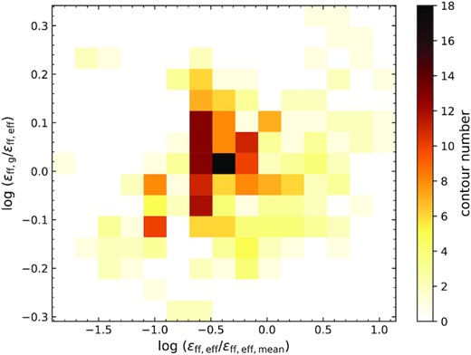
2D distribution plot of (ϵff,g/ϵff,eff) versus (ϵff,eff/ϵff,eff,mean). The values are determined from simulation contours, and the colour shows the number of contours in each bin.
3.2 Application to Herschel observations
The first step in applying our method to the Herschel observations is to generate column-density contours across the full range of |$N(\rm H_2)$| covered by the observations. For each of the 12 regions, we start by finding the lowest |$N(\rm H_2)$| value such that all pixels with column density above it are inside the SESNA coverage; equivalently, we set the minimum value of |$N(\rm H_2)$| to be the lowest possible choice such that the contour sits entirely within the SENSA footprint. We define M0 as the total gas mass enclosed by this contour. We then draw 100 |$N(\rm H_2)$| contours at higher |$N(\rm H_2)$|, with the levels chosen such that the total mass above each level is equally spaced from M0 to M0/100 with a step of M0/100; we only retain contours that contain at least one protostar, consistent with the selection we apply to the simulations in H21. We show an example of Ophiuchus cloud column-density map with |$N(\rm H_2)$| contours, protostar positions, and SESNA coverage area in Fig. 2.
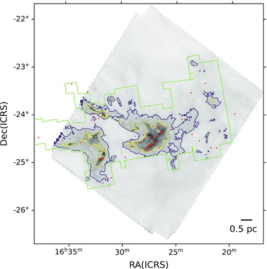
A column-density map of the Ophiuchus cloud derived from Herschel observations. The green contour is the Spitzer coverage area, and we illustrate the largest contour that fits within this footprint in purple; the yellow contour is set at a level that encloses half as much mass as the purple one. The red dots are the positions of protostars.
For every contour, we measure four values: total gas mass Mgas, total area A, completeness-corrected total protostar number NPS, and the Gini coefficient g of the surface density of all pixels within the contour (see H21 for details). From these parameters, we derive five additional quantities: mean gas surface density Σgas = Mgas/A, star-formation surface density ΣSFR, the volume density ρsph, and free-fall time derived from the spherical assumption tff,sph (see Section 1), and the corresponding star-formation efficiency per free-fall time ϵff,sph. To calculate ΣSFR, we assume the mean mass of protostars in SESNA to be MPS ≈ 0.5 M⊙ (Evans et al. 2009), and the mean duration of protostellar phase included in SESNA observations to be tPS ≈ 0.5 Myr (Dunham et al. 2014, 2015). Thus, ΣSFR = NPSMPS/AtPS, and ϵff,sph = ΣSFR/(Σgas/tff,sph).
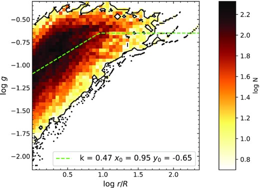
2D distribution plot of g versus log (r/R). The values are determined from the smeared contours, and the colour shows the number of contours in each bin (one black dot represents one single contour). The green dash line shows the piece-wise function equation (3) fitted to this distribution.
We perform a similar analysis to control for the effects of the limited dynamic range of the observations, i.e. the fact that there are minimum and maximum measurable values of Σgas, and this in turn imposes limits on the maximum possible value of g. Define η = Σgas,min/Σgas,max < 1 as the ratio of minimum and maximum column densities within a given map contour. The value of η necessarily limits the range of g, since as η → 1, the column densities within the contour all become the same, and clearly we must therefore have g → 0.
We can use this result to study where limited dynamic range begins to affect our results by examining the locations of our contours in the (η, g) plane – contours that lie near the upper limit suggest that our measured values of g may be compromised by limited dynamic range, while those that lie well below the limit are likely to suffer only minimal effects.
We plot 2D histograms of g versus log η for both our Herschel observations and for the C18 simulations, together with equation (4), in Fig. 4. We see that, for both the simulations and observations, the distribution approaches the limit as η → 1, but falls significantly below it when η ≪ 1. Based on this figure, we choose to truncate our sample at log ηmax = −0.7, since for both the simulations and the observations the data approach the maximum value of g for log η > −0.7, but fall well below it for smaller η.
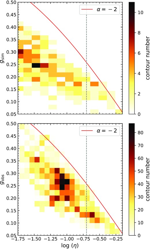
2D histograms of contour Gini coefficients g and column-density range log (η). Top panel: Simulation contours. Bottom panel: Herschel map contours. The solid line plots in both panels show the theoretical value of g for contours with perfect power-law column-density distributions with α = −2 (equation 4), the approximate value we measure in both simulations and observations; results for other values of α within the uncertainty of the fits are nearly indistinguishable. The grey dashed vertical line shows log (η) = −0.7. Note that the simulations, which have greater dynamic range than the observations, extend well beyond the range of η shown in the plot.
To ensure that our truncation of the sample at both small radii and small dynamic range does not create an inconsistency between the observations and our simulations, we apply the same cuts to the simulations and refit the relationship between ρeff, ρsph, and g, using the same method as described in H21. Doing so yields k = 4.3 ± 0.1, b = 0.84 ± 0.04, and a coefficient of determination R2 = 0.70. The error range of k and b are obtained from half-sample fitting as described in Section 3.1. Such values are close to previous ones. For consistency, we will use the new fitted model coefficients throughout the rest of this manuscript.
Applying the down-selections described above to the Herschel data, we obtain 2905 contours that form the data set for further analysis. For all selected contours, we apply equation (2) (with the modified values of k and b) to determine their effective volume density ρg, and replace |$\rho _{\rm _sph}$| with ρg to recalculate the new result star-formation efficiency denoted as ϵff,g.
4 RESULTS
With the properties determined from the unsmeared contours on different surface-density levels, we first investigate how the triplet (g, ϵff,sph, ϵff,g) changes with Σgas. In Fig. 5, we show the 2D histogram of g versus log (Σgas). We can find no significant relation between g and Σgas in this plot, which is consistent with the simulation results. The median value of g is gmedian = 0.24, which is above 0.2, the value for a uniform-density sphere (H21). This indicates that the free-fall time of most contours will be overestimated by the spherical assumption. For a typical Gini coefficient g = 0.24, our estimated uncertainties on k and b in equation (2) translate to an increase in the dispersion of ϵff by 0.01 dex, which is negligible. For this reason, we will simply treat k and b as constants fixed to their central values for the remainder of this analysis. Similarly, given that we have an average of 300 contours per cloud, the 0.18 dex mean residual scatter of the H21 model corresponds to only a ∼0.005 dex scatter in the percentiles and mean values of ϵff, negligibly small.
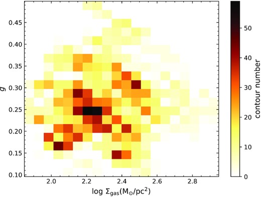
2D histogram plot of g versus log (Σgas). The values are determined from the unsmeared contours after all selections, and the colour shows the number of contours in the bin.

Distributions of log ϵff,sph (top panel) and log ϵff,g (bottom panel) as a function of log Σgas. For each cloud, the coloured line and grey band show the 50th percentile and 16–84th percentile range of ϵff in a bin of log Σgas. The black dashed lines show the median values 〈ϵff,sph〉 and 〈ϵff,g〉 over all clouds.
We report the 〈ϵff〉 and σ values we measure using the spherical assumption (denoted by subscript sph) and with equation (2) (subscript g) for all 12 clouds in Table 1. After applying our model, the median value of log 〈ϵff〉 decreases from log〈ϵff,sph〉 = −1.73 to log 〈ϵff,sph〉 = −1.90. This is consistent with the prediction in H21 that use of the spherical assumption leads to a ∼0.13 dex overestimation of ϵff. We also measure the difference in dispersion Δσ = σsph − σg derived using the spherical assumption versus using equation (2) for each cloud. We find that eight of the 12 studied clouds yield positive Δσ, corresponding to a reduction in the dispersion; the mean reduction is Δσmean = 0.02 dex. This demonstrates that our model does decrease the dispersion, but less than the ∼0.15 dex found when testing the method on simulated data in H21. This is likely due to the difference between the simulated data and observations. H21 calibrate their method based on simulations from Cunningham et al. (2018) that use periodic boundary conditions, so the column-density maps used in the calibration are from infinitely large self-similar clouds. The observed clouds, however, are from of finite size, so, for example, they can contain large-scale density gradients that are absent in periodic boxes. This suggests that we might obtain an improved version of equation (2) by analysing a zoom-in galactic simulation.
Estimates of 〈ϵff〉 and σ for individual clouds, using both the spherical assumption (values with subscript ‘sph’) and the Gini model equation (2) (values with subscript ‘g’); Δσ = σsph − σg. The column log Σgas reports the (min, max) contour average surface density measured for each cloud. Finally, the last three rows list the median, mean, and standard deviation (STD) values of the corresponding columns.
| Cloud | log〈ϵff,sph〉 | log〈ϵff,g〉 | σsph | σg | Δσ | log Σgas |
|---|---|---|---|---|---|---|
| (dex) | (dex) | (dex) | (|$\rm M_{\odot }\,pc^{-2}$|) | |||
| Ophiuchus | −1.45 | −1.59 | 0.18 | 0.13 | 0.05 | (2.05, 2.79) |
| Persus | −1.76 | −1.97 | 0.28 | 0.31 | −0.03 | (1.85, 2.67) |
| Orion-A | −2.12 | −2.29 | 0.13 | 0.15 | −0.02 | (2.24, 3.00) |
| Orion-B | −1.86 | −2.03 | 0.19 | 0.16 | 0.03 | (2.10, 2.64) |
| Aquila-N | −1.79 | −2.03 | 0.31 | 0.23 | 0.08 | (2.02, 2.56) |
| Aquila-S | −1.69 | −1.84 | 0.18 | 0.11 | 0.07 | (1.92, 2.78) |
| NGC 2264 | −1.84 | −2.18 | 0.04 | 0.05 | −0.01 | (1.97, 2.77) |
| S140 | −1.62 | −1.78 | 0.04 | 0.03 | 0.01 | (1.95, 2.36) |
| AFGL 490 | −1.45 | −1.56 | 0.01 | 0.00 | 0.01 | (2.14, 2.32) |
| Cep OB3 | −1.76 | −1.82 | 0.13 | 0.11 | 0.02 | (1.92, 2.41) |
| Mon R2 | −1.69 | −1.97 | 0.06 | 0.09 | −0.03 | (1.77, 2.48) |
| Cygnus-X | −1.63 | −1.67 | 0.41 | 0.40 | 0.01 | (1.90, 2.78) |
| Median | −1.73 | −1.90 | 0.16 | 0.12 | 0.01 | – |
| Mean | −1.72 | −1.89 | 0.16 | 0.15 | 0.02 | – |
| STD | 0.18 | 0.22 | – | – | – | – |
For all 12 clouds, we determine the STDs of both types of 〈ϵff〉 values: STDsph = 0.18, and STDg = 0.22. There is a slight increase after applying the H21 model, the reason for which might be that there are real physical differences between clouds that we have uncovered by not adopting the uniform spherical assumption. Given the relatively small Δσmedian we obtain, it is also interesting to ask whether we could forgo individualized corrections altogether, and simply adopt the median value g = 0.24 for all contours. Doing so would still produce a 0.1 dex median value decrease in ϵff, while leaving the dispersion unchanged. However, such an approach would miss an important subtlety: while g = 0.24 is the median value for all contours on all scales, the value of g also changes systematically with size scale: on the largest scales of the 12 clouds we study, gmedian = 0.35. Properly accounting for this is crucial to obtaining the correct changes in ϵff versus Σgas, and thus the correct Δσ values within individual clouds. For this reason, we prefer to use individual-contour corrections when possible.
5 CONCLUSIONS
We use a new method proposed by H21 to combine column-density maps derived from Herschel with YSOs from the SESNA catalogue to determine the star-formation efficiency per free-fall time ϵff in 12 nearby clouds. Our method provides a more realistic estimate of the mean volume densities of clouds seen in projection, reducing the error incurred by assuming that projected clouds are spherical, and allowing higher precision estimates of ϵff than previously possible. We find that the spherical assumption leads to ∼0.1 dex overestimation of log 〈ϵff〉, and also increases the estimated intracloud dispersion in log 〈ϵff〉 by ∼0.02 dex on average. With our new method, we find that our sample of 12 clouds has a median star-formation efficiency per free-fall time log 〈ϵff〉 = −1.9, and the median spread in log 〈ϵff〉 = 0.12 dex within a single cloud. The intercloud dispersion in log 〈ϵff〉 is nearly identical, at 0.2 dex, and this value is, within the uncertainties, unaffected by the use of the H21 model for the gas density. This strongly suggests that the intracloud dispersion we are measuring reflects a real variation in cloud properties, not an observational error.
Our results confirm the existence of a universal ϵff ∼ 0.01 value, and, importantly, let us identify a real ≈0.2 dex spread from cloud to cloud with 3D cloud geometry considered for the first time. As discussed in Pokhrel et al. (2021), such a small spread is in tension with models where star formation is regulated mainly by galactic-scale processes, but individual molecular clouds undergo rapid collapse (e.g. Kim et al. 2011; Ostriker & Shetty 2011; Faucher-Giguére et al. 2013). These models predict a much larger dispersion. Conversely, however, our measured spread in ϵff can be used to evaluate the spread in parameters that enter models for cloud-scale regulation of star formation, which do predict dispersions comparable in size to the observed one. For example, in the turbulence-regulated star formation of Krumholz & McKee (2005), a ∼0.2 dex spread in ϵff could naturally be explained by a σα ∼ 0.3 dex spread in cloud virial parameters (or a |$\sigma _{\mathcal {M}}\sim 0.7$| dex spread in Mach number), while in the similar model of Hennebelle & Chabrier (2011) the required dispersion is σα ∼ 0.8 dex (|$\sigma _{\mathit {M}} \sim 0.6$| dex), and for the model of Padoan et al. (2012) would require σα ∼ 0.5 dex. For comparison, Lee et al. (2016) study 195 star-forming giant molecular clouds and find a scatter of 0.32 dex in the virial parameter. Thus, observed clouds have approximately the level of dispersion in virial parameter required to reproduce the spread we see in ϵff. In future work, we can use the same technique of high-precision estimates of ϵff deployed here to search not just for the dispersion in ϵff, but to look for systematic variations with virial parameter or other cloud properties, thereby opening up a new method for testing theories of star formation.
ACKNOWLEDGEMENTS
We acknowledge the anonymous referee for the insightful advice on this manuscript. M. R. K. acknowledges funding from Australian Research Council awards DP190101258 and FT180100375. R. P. and R. A. G. acknowledge support from National Aeronautics and Space Administration (NASA) Astrophysics Data Analysis Program (ADAP) awards NNX15AF05G, 80NSSC18K1564, and NNX17AF24G. R. P. acknowledges funding from NASA ADAP award 80NSSC18K1564, and R. A. G. acknowledges funding from NASA ADAP awards NNX11AD14G and NNX13AF08G. We further acknowledge high-performance computing resources provided by the Australian National Computational Infrastructure (grants jh2 and ek9) through the National and Australian National University (ANU) Computational Merit Allocation Schemes, and by the Leibniz Rechenzentrum and the Gauss Centre for Supercomputing (grant pr32lo).
This research has made use of data from the Herschel Gould Belt survey (HGBS) project, a Herschel Key Programme jointly carried out by SPIRE Specialist Astronomy Group 3 (SAG 3), scientists of several institutes in the PACS Consortium (CEA Saclay, INAF-IFSI Rome, and INAF-Arcetri, KU Leuven, MPIA Heidelberg), and scientists of the Herschel Science Center (HSC).
DATA AVAILABILITY
The data underlying this article will be shared upon reasonable request to the corresponding author.
