


ABSTRACT
Pulsar wind nebulae (PWNe) represent the largest class of sources that upcoming γ-ray surveys will detect. Therefore, accurate modelling of their global emission properties is one of the most urgent problems in high-energy astrophysics. Correctly characterizing these dominant objects is a needed step to allow γ-ray surveys to detect fainter sources, investigate the signatures of cosmic ray propagation, and estimate the diffuse emission in the Galaxy. In this paper, we present an observationally motivated construction of the Galactic PWNe population. We made use of a modified one-zone model to evolve for a long period of time the entire population. The model provides, for every source, at any age, a simplified description of the dynamical and spectral evolution. The long-term effects of the reverberation phase on the spectral evolution are described, for the first time, based on physically motivated prescriptions for the evolution of the nebular radius supported by numerical studies. This effort tries to solve one of the most critical aspects of one-zone modelling, namely the typical overcompression of the nebula during the reverberation phase, resulting in a strong modification of its spectral properties at all frequencies. We compare the emission properties of our synthetic PWNe population with the most updated catalogues of TeV Galactic sources. We find that the firmly identified and candidate PWNe sum up to about 50 per cent of the expected objects in this class above threshold for detection. Finally, we estimate that Cherenkov Telescope Array will increase the number of TeV-detected PWNe by a factor of ≳3.
1 INTRODUCTION
A pulsar wind nebula (PWN) is a relativistic bubble generated by the interaction of the wind from a rotating neutron star, the pulsar (PSR), with the surrounding ambient medium. In young systems, the latter is formed by the debris from the explosion of the progenitor star, the supernova ejecta. As the pulsar spins down, losing rotational energy, the largest part of it is converted into a relativistically expanding, magnetized outflow, mainly – if not totally – composed by electron–positron pairs: the pulsar wind. In order to match the boundary conditions of the slowly expanding supernova ejecta, this wind is forced to slow down at a strong magneto-hydrodynamic (MHD) termination shock, where the plasma is heated and potentially strong magnetic dissipation takes place (for a review, see e.g. Gaensler & Slane 2006). The same shock is also thought to be the place for particle acceleration, with evidence for leptons accelerated up to PeV energies in the Crab nebula (Arons 2012; Amato 2014; Bühler & Blandford 2014).
A PWN shines in a broad range of energies from radio to γ-rays. The lower energy emission – up to about 100–200 MeV (for young PWNe, with magnetic fields in the 100-μG range) – is typically the result of synchrotron radiation by particles interacting with the nebular magnetic field. The energy-dependent size of many PWNe reflects the fact that higher energy particles have shorter lifetimes against radiation losses and thus survive on shorter distances from their injection location at the shock. The synchrotron emission is often highly polarized (Novick et al. 1972; Weisskopf et al. 1978; Velusamy 1985) in a way that suggests that the magnetic field in the inner regions is mostly toroidal (Kennel & Coroniti 1984) and ordered to a high degree. Finally, in terms of morphology, the well-known X-ray jet-torus shape identified in the inner region of several PWNe (Weisskopf et al. 2000; Gaensler, Pivovaroff & Garmire 2001; Helfand, Gotthelf & Halpern 2001; Gaensler et al. 2002; Lu et al. 2002; Pavlov et al. 2003) is interpreted as due to the anisotropic energy injection from the pulsar wind.
At frequencies larger than the synchrotron cutoff, the PWN emits radiation via inverse Compton scattering (ICS) of electrons and positrons on the local radiation fields: the background of synchrotron photons; the cosmic microwave background (CMB); infrared (IR) thermal photons from the local dust; and photons coming from background stars. At TeV energies, the major contributors to the ICS emission are the relatively low-energy leptons responsible for radio-IR synchrotron emission. Since these have longer radiation lifetimes than the X-ray emitting particles, a PWN will then remain bright in very high-energy γ-rays even when the X-ray emission has completely faded away. The lifetime of a γ-ray PWN, between 100 GeV and 300 TeV, can be estimated to be ∼50−100 kyr. Considering an expected birth rate of pulsars in the Galaxy of ≃1/100 yr (Faucher-Giguère & Kaspi 2006), one can naively estimate around ∼500−1000 γ-ray-emitting PWNe. This means that, among the many classes of Galactic γ-ray-emitting sources, PWNe are likely to be the most numerous. As a consequence, their identification/discrimination will be one of the biggest challenges in the analysis of the data obtained by the next generation of γ-ray instruments, such as the Cherenkov Telescope Array (CTA). In fact, most of the newly detected γ-ray PWNe will not have any associated lower energy emission to guide their identification. Already in the H.E.S.S. Galactic Plane Survey (HGPS hereafter), out of 24 extended sources, for which a PWN has been invoked, only 14 have been firmly identified with known objects, with the remaining 10 having no clear counterpart at other wavelengths (Abdalla et al. 2018b).
Typically, the two preferred ways to identify a TeV source as a PWN are: (i) the detection of a spatially coincident PWN at lower energies (Kargaltsev, Rangelov & Pavlov 2013); (ii) the co-location of a pulsar in the TeV-emitting area. The latter strategy is applicable only to a fraction of the sources, since the pulsar can be seen directly only when its beamed radiation intercepts our line of sight. The multiwavelength association is then usually preferred for a firm identification. For statistical reasons, related to the larger number of older objects, most of the γ-rays from PWNe will come from evolved systems, whose X-ray emission has long faded away, and whose radio emission is weak and extended, difficult to detect on top of the background. Devising an effective strategy to identify these systems is a problem of increasing urgency as the operational phase of CTA approaches. Some efforts to develop reliable models to establish more safely the possible associations are starting to be made (Olmi & Torres 2020).
In this work, we present the first attempt to reproduce the population of γ-ray-emitting PWNe based on state-of-the-art modelling of the PWN evolution and on current knowledge of the pulsar population and associated Supernova Remnants (SNRs). The two main novelties of our approach with respect to analogous efforts in the literature are: (1) a revised, physically informed, one-zone treatment of the evolution and radiation properties of these systems; (2) the adoption of a population of Galactic pulsars selected based on γ-ray data, so as to be representative of young enough objects to power-observable nebulae. It is worth pointing out that we simulate the evolution of each system individually, in contrast with previous studies (e.g. Abdalla et al. 2018b), where a single ‘average’ source was considered and its parameters varied so as to match the observed population of TeV-emitting PWNe. We compare the predictions for the γ-ray emission from our entire synthetic population of PWNe with observational results from the HGPS and extract global trends. While also VERITAS (Aliu et al. 2013a, 2014; Mukherjee & VERITAS Collaboration 2016) and MAGIC (Anderhub et al. 2010; Rico 2016) have greatly contributed to improve our knowledge of PWNe at TeV photon energies, our choice of the HGPS as a reference is due to the fact that this provides the most complete available survey of these sources, comprehensive of all but one (J1831-098) of the PWNe reported in TeVcat.1 Before concluding, we also briefly discuss how the advent of CTA is expected to further improve our current knowledge of these systems.
The paper is organized as follows: in Section 2, we describe and discuss the assumptions at the basis of the PWN population model; in Section 3, we present the numerical tools used to generate the synthetic population and its complete spectral evolution; and in Section 4, we discuss our results and compare with observations available from the HGPS. Finally, in Section 5, we draw our conclusions and comment on possible further developments of the model.
2 GENERATING THE POPULATION
An observationally motivated model of the γ-ray-emitting PWNe in the Galaxy must take into account the following aspects:
the distribution of core collapse SNRs in the Galaxy;
a population of pulsars able to account for the formation of newborn PWNe;
the association of each pulsar with a core collapse SNR;
the evolution of PWNe from birth to the late stages.
For the synthetic population of Galactic SNRs, we have used the one presented in Cristofari et al. (2017), which had been optimized for reproducing the γ-ray SNRs of the Galaxy. In that work, the authors located core collapse (CC hereafter) SNRs according to the spatial distribution of Galactic pulsars as modelled by Faucher-Giguère & Kaspi (2006) (FGK06 hereafter). The rate of supernova explosions is taken to be 3 per 100 yr. Each remnant has an associated energy Esn = 1051 erg, which is generally assumed as a representative value (see, however, Hamuy 2002; Nadyozhin 2003; Zampieri et al. 2003; Müller et al. 2017 for the variability of CC supernova energetics). Cristofari et al. (2017) considered a wide range of densities for the interstellar medium (ISM) (10−5–10 particles cm−3), with the spatial distribution taken from Nakanishi & Sofue (2003), Nakanishi & Sofue (2006). CC SNR masses are taken from a Gaussian distribution peaking at |$13\, M_\odot$|, with |$\sigma =3\, M_\odot$| (a summary of all the parameters needed to generate the population is reported in Table B1). The distribution is cut at a minimum value of |$5\, M_\odot$| and the maximum one is imposed to be |$20\, M_\odot$|, with those systems having Mej > 20M⊙ reset to |$M_\mathrm{ej}=20\, M_\odot$| (Smartt 2009). The latter choice is somewhat arbitrary, but given the lack of information on the distribution of Mej among the PWNe population, we decided to adopt the simplest approach to enforce the upper limit suggested by Smartt (2009). In any case, this choice affected a relatively small fraction of the entire sample (|$\lesssim 8{{\ \rm per\ cent}}$|). The spatial distribution of the considered CC SNRs in the Galaxy, as well as ejecta mass distribution, is shown in the left-hand panel of Fig. 1.
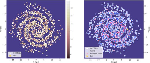
Left-hand panel: Reference population of the Galactic core collapse (CC) SNRs. The distribution of the ejecta masses (in units of solar mass) is colour coded as indicated in the colour bar. Right-hand panel: The PWNe population on top of CC SNRs. Pink circles mark runaway PSRs that, at the end of their evolution, have left their parent SNR bubble, while blue circles are for systems that remain inside the remnant during the entire evolution. In both plots, the Sun position is marked with a yellow star and the Galactic coordinates are expressed in kpc.
To produce the synthetic population of Galactic PWNe, we have then to associate a pulsar to each CC SNR of the sample. A possibility would be to use the pulsar population described in FGK06, defined on the basis of the observations of Galactic radio-emitting pulsars. This population, however, is clearly dominated by evolved objects (namely PSRs with characteristic ages typical of rotation-powered radio pulsars, roughly in the range of 1–20 Myr), by construction, and thus appears not to be the best choice in the present context, where the intent is that of simulating PWN powering, and hence young (age ≲1 Myr), pulsars.
We considered more appropriate for the present scope to adopt the population of the γ-ray-emitting pulsars that trace mostly young neutron stars. In particular, we chose the one described in Watters & Romani (2011) (WR11 hereafter), also similar to the one recently presented by Johnston et al. (2020). To evaluate the impact of this choice on the final results, we run our model with different recipes for the pulsar population and compared the results with available γ-ray data. We will discuss this point in more detail later in this section.
The validity of our assumption that γ-ray pulsars well represent the young population of pulsars powering PWNe in the Galaxy has been verified by running multiple simulations of the entire population, varying the distribution of initial spin-down periods P0. In particular, we considered four different possibilities: pure FGK06 (centred at 300 ms), pure WR11 (centred at 50 ms), and two intermediate populations, the first one with P0 centred at 80 ms and the second with P0 centred at 120 ms. For all these cases, we computed the γ-ray emission and then compared the results with the available γ-ray data, as taken from the gamma-cat catalogue.2 We found that the PWN population based on the WR11 pulsar distribution is the one that best reproduces the available observations. In all the other cases, the resulting γ-ray flux exceeds the observed one.
We associate a three-dimensional (3D) kick velocity to each pulsar of the population, considering the double-sided exponential velocity distribution model of FGK06, with a mean value of ∼380 km s−1. Since SNRs are in decelerated expansion in the ambient medium, a large fraction of all the pulsars are actually expected to escape from the bubble of their parent SNR on time-scales comparable with the final age considered for this work and then to form bow shock pulsar wind nebulae (BSPWNe) shaped by the interaction with the ISM (Bucciantini 2002; van der Swaluw et al. 2003; Bucciantini, Amato & Del Zanna 2005; Vigelius et al. 2007; Kargaltsev et al. 2017; Barkov, Lyutikov & Khangulyan 2019; Olmi & Bucciantini 2019a; Toropina, Romanova & Lovelace 2019). BSPWNe are perfect locations where to look for efficient particles escape (Olmi & Bucciantini 2019c), and associated TeV haloes (Abeysekara 2017; Sudoh, Linden & Beacom 2019). The population of PSRs and associated SNRs is generated using a Monte Carlo technique and assuming no correlation among the various parameters describing the system. This produces the initial synthetic population of PWNe shown in the left-hand panel of Fig. 1, where we also highlight the PSRs escaped from their parent remnants at the end of the simulation.
In Fig. 2, we compare our synthetic population both with all the pulsars from the ATNF (Australia Telescope National Facility) catalogue3 and with those having an associated PWN, either from the HGPS or from other independent observations (Aharonian et al. 2004, 2005,2006; Abramowski et al. 2012, 2015; Aliu et al. 2013b; Aleksić et al. 2014). Our population is limited to systems with age younger than tend = 105 yr, which translates into a cut in our synthetic sample, as can be clearly seen in Fig. 2. We have verified, however, by varying the final age that this does not affect the results of the present study, given that for older PSRs the γ-ray luminosity of the associated PWN is negligible. In the distribution of luminosities versus characteristic ages, we also compare the baseline model from the PWNe analysis in the HGPS [red dashed line – see equation (5) of Abdalla et al. 2018b] with that computed using the median values of L0 and τ0 from our synthetic population. It is noteworthy that the two appear very close together, despite the simplified assumption, and limited number of objects, used to build the baseline model in Abdalla et al. (2018b).
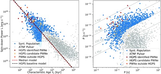
Some characteristic quantities of the chosen population of pulsars (blue circles) to be directly compared with similar plots from Abdalla et al. (2018b) (see e.g. their Fig. 2). The other symbols in the plot represent: PSRs powering PWNe that are firmly identified in the HGPS (red squares); PSRs possibly associated with candidate HGPS PWNe (yellow circles); the five PSRs powering nebulae that are included in the HGPS plots as outside HGPS PWNe (orange diamonds), because the associated PWNe are outside the HGPS field, or have not been analysed with the HGPS pipeline (see Abdalla et al. (2018b) for details); all other pulsars from the ATNF catalogue (grey dots). Left-hand panel: distribution of the pulsars in the characteristic age–luminosity diagram. Dashed lines represent the median of our distribution (red) and the HGPS baseline model (black). Right-hand panel: distribution of synthetic pulsars in the spin-down period–spin-down period derivative (P-|$\dot{P}$|) diagram. Dashed lines indicate different characteristic ages of the sources in the population.
3 EVOLVING THE POPULATION
Typically, our population contains ∼1300 sources, which are all evolved up to the final age of tend = 105 yr. To model the spectral and dynamical evolution of each PWN, we adopt the so-called one-zone approach (Venter & de Jager 2007; Zhang, Chen & Fang 2008; Gelfand, Slane & Zhang 2009; Qiao, Zhang & Fang 2009; Fang & Zhang 2010; Tanaka & Takahara 2010, 2011; Bucciantini, Arons & Amato 2011; Martín, Torres & Rea 2012; Torres et al. 2014b; Martín, Torres & Pedaletti 2016; van Rensburg, Krüger & Venter 2018; Zhu, Zhang & Fang 2018; Fiori et al. 2020). This approach has been widely and successfully applied to systems of different ages and allows one to rapidly model the full evolution, even for very old systems. With current computational capabilities, this is not feasible with more sophisticated one-dimensional (1D) or multidimensional approaches based on hydrodynamic (HD) or even MHD numerical simulations (Blondin, Chevalier & Frierson 2001; van der Swaluw et al. 2001; Komissarov & Lyubarsky 2004; Del Zanna et al. 2006; Porth, Komissarov & Keppens 2014a; Olmi et al. 2016; Olmi & Torres 2020). In addition, there are physical reasons to believe that one-zone models might provide a better description of the system than reduced dimensionality MHD simulations: in fact, 1D and two-dimensional (2D) MHD models fail to capture the important role that turbulence and mixing are bound to play in the late PWN dynamics (see e.g. the discussion on the differences of 2D and 3D dynamics in Porth et al. 2014a or Olmi et al. 2016).
In one-zone models, the PWN is treated as a homogeneous system, whose evolution is governed by the interaction with the surrounding SNR and by particles and energy losses (both adiabatic and radiative). In particular, the PWN radius is treated as coincident with that of the thin and massive shell of swept-up material that accumulates at the PWN boundary as it expands, initially in the un-shocked ejecta and later on in the SNR shell (van der Swaluw et al. 2001; Bucciantini et al. 2003; Gelfand et al. 2009; Martín et al. 2012). The one-zone approach was used multiple times in the past, and it was proved to give robust results, at least in describing the first phase of the evolution, when the PWN expands with mild acceleration within the freely expanding SNR. Recently, Bandiera et al. (2020) have shown that those models must be used with caution when addressing longer evolution time-scales and passing through the phase known as reverberation. The reverberation phase begins when the SNR reverse shock (RS hereafter), that moves from the border of the SNR towards the centre, reaches the boundary of the PWN bubble. Depending on the energetics of the PWN and the pressure in the SNR, this interaction may cause a series of contractions and re-expansions of the PWN, which possibly affect its spectral and morphological properties. The effects of the modifications induced by the reverberation are usually quantified through the so-called compression factor (cf), namely the ratio between the maximum radius of the PWN – reached in the early reverberation phase, before the PWN starts contracting – and the minimum one – namely that when the PWN is maximally compressed. A dramatic modification of the spectral properties of a PWN, called super-efficiency, was described by Torres, Lin & Coti Zelati (2019), who found very large compression factors, up to cf > 1000. In these extreme cases, the particle heating and the enhancement of the nebular magnetic field are so huge as to cause catastrophic synchrotron losses, strongly reducing the number of particles available for ICS emission at late times. More recently, Bandiera et al. (2020) have shown that this super-efficiency phase might actually be expected only for a small fraction of the PWNe population, while most of the systems will experience a maximum compression of a few tens, which will not reflect in such a drastic modification of the spectral properties at all wavelengths. The possibility of strong compressions and later re-expansions during the reverberation phase had been first criticized by Bucciantini et al. (2011) and is the subject of an ongoing study of some of the authors of the present manuscript. Current results indicate that the thin-shell approximation is not accurate enough when looking at the PWN properties close to the reverberation phase and leads to overestimate the compression (Bandiera et al. 2020 and Bandiera et al., in preparation).
Of course, a realistic and detailed description of the PWN–SNR co-evolution requires much more sophisticated modelling. 3D MHD simulations offer the minimum degree of complexity that still allows to account for essential phenomena, such as magnetic instabilities and dissipation (which may reduce the magnetic field enhancement during compression) and fluid instabilities (like Rayleigh-Taylor’s) that might develop at the contact discontinuity and partly or completely disrupt the thin shell (Blondin et al. 2001; Bucciantini et al. 2004; Porth, Komissarov & Keppens 2014b; Kolb et al. 2017; Olmi & Torres 2020), hence strongly reducing the compression during the reverberation phase. However, a 3D MHD investigation, up to very late times, is beyond current computational possibilities. 3D models of young PWNe have shown to require millions of CPU hours and months of continuously running computations for reproducing only a limited part of their evolution (Porth et al. 2014a; Olmi et al. 2016). They have been then used to investigate only a limited number of sources. Moreover, these models still lack a consistent treatment of radiative losses, generally traced in the post-processing and not directly linked to the evolution (see e.g. Komissarov 2004; Del Zanna et al. 2006; Olmi et al. 2013).
On the other hand, MHD simulations of reduced dimensionality are likely to provide an inaccurate description of the internal dynamics of the system (see e.g. the discussion in Olmi & Torres 2020), which in this context reflects in a poor description of the evolution during the most dramatic phases of the interaction between the PWN and the SNR reverse shock. In light of recent and current investigations (Bandiera et al. 2020, 2021 and Bandiera et al. in preparation), we believe that one-zone models, with complete neglect of the internal dynamics and an informed prescription for the evolution of the nebular radius, provide more reliable results for the long-term evolution of the system than reduced dimensionality MHD models.
3.1 Dynamical evolution
3.1.1 Free-expansion phase
The pressure in the relativistic and homogeneous bubble that approximates the PWN is given by the sum of the magnetic pressure and the pressure of the relativistic particles, whose energetic evolves taking into account energy injection from the PSR as well as adiabatic and radiation losses (see Section 3.2).
3.1.2 Reverberation phase
This approach represents a substantial improvement with respect to simply assuming a pressure proportional to the Sedov solution (see e.g. Gelfand et al. 2009; Torres et al. 2014b), and we have found it adequate to the aims of the present work, namely to obtain predictions of the statistics of the broad-band emission, with a special focus on the TeV range. A more sophisticated analysis, with a larger set of 1D models, is underway and results will be published in a forthcoming paper.
3.1.3 Relic phase: BSPWNe, old PWNe, and leftover bubbles
More relevant for the present work is the role of the relic bubbles of electrons injected in the nebula during the PSR history. Among these particles, the lowest energy ones, producing radio synchrotron radiation, will not have cooled down by the time the PSR escapes the SNR or moves outside of the original wind bubble (which usually happens earlier than tesc), so that these systems are possible sources of ICS γ-ray emission. The escape of the PSR from its original wind bubble, proven by the existence of highly asymmetric systems, is a problem with which all one-zone models struggle to deal (Gelfand et al. 2009). Starting from the time the PSR escapes, the nebula of leftover electrons is treated as a relic subject to adiabatic expansion alone. We will come back to this point at the end of Section 4, with a more quantitative discussion.
3.2 Spectral evolution
In Fig. 3, we show the expected photon spectral evolution for one of our sources during each of the characteristic phases that have been previously described in Section 3.1. The evolution of the PWN radius and magnetic field strength is also shown. The corresponding input parameters are listed in Table 1. During the free-expansion phase, the synchrotron emission, extending from the radio band up to a few tens (or even hundreds for the brightest sources) of MeV, decreases with time. The MeV cutoff moves to lower energy, due to the decreasing magnetic field. Similarly, the break between radio and optical wavelengths, which reflects the break in the injected particle population, moves to lower energy. Due to the fading of the magnetic field during this phase, the synchrotron cooling break moves to higher frequencies (being B ∝ t−p with p ≥ 1 and νB ∝ B−3t−2 ∝ t3p − 2). In this model, characterized by a large τ0 (τ0 > tch), so that particles are efficiently injected during all the free-expansion phase, this implies that particles injected at later times are less affected by synchrotron losses. This causes a progressive hardening of the X-ray spectrum during this phase and also the ICS emission to peak at increasingly higher energies. The change of the main target radiation from the CMB to the IR-optical, which has a larger energy density, also leads to an overall enhancement of the ICS emission. The observed decrease with time of the maximum frequency at which synchrotron radiation is emitted reflects the fact that in this particular system, acceleration is never radiation limited and the maximum energy is set to the pulsar potential drop. Once the system enters the first reverberation phase, and starts experiencing compression, the trend of synchrotron emission is reversed: the MeV cutoff and the radio-optical break move to higher energies; the total synchrotron luminosity increases, and now the combination of synchrotron cooling and adiabatic gains leads to a very steep spectrum in the optical to X-ray range (Bucciantini et al. 2011). The ICS emission keeps rising, but now it peaks at progressively lower energies, due to the burn-off of the electrons able to interact with more energetic photons than the CMB ones. After the compression phase, the system experiences a re-expansion. The various spectral features of the synchrotron portion of the spectrum change in a similar way to the initial phase of free expansion. The latest phases of evolution show a more structured ICS spectrum, with a shape that depends on the properties of the synchrotron spectrum at the moment the PWN enters the reverberation process.
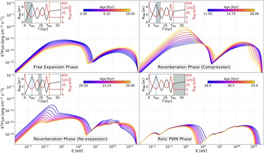
Spectral evolution of a (randomly extracted) source in the modelled population during different evolutionary phases. In all panels, a sub-panel illustrates the evolution of the radius (in black) and of the magnetic field (in red) with time, from 0 to the time at which the PSR eventually escapes from the SNR bubble (TREL). Notice that the magnetic field in the relic stage is not zero but fixed to 5 μG. The grey area in the sub-panels highlights the stage at which the spectra in each panel are extracted. The exact time to which each of the plotted spectra corresponds can be read from the colour bar.
Parameters of the source illustrated in Fig. 3.
| Parameter | Symbol | Our source |
|---|---|---|
| Braking index | n | 3 |
| Initial spin-down age (yr) | τ0 | 19 971 |
| Initial spin-down luminosity (erg s−1) | L0 | 2.26 × 1036 |
| SNR-ejected mass (M⊙) | Mej | 18.60 |
| Energy break (TeV) | Eb | 0.23 |
| Low energy index | α1 | 1.25 |
| High energy index | α2 | 2.49 |
| Magnetic fraction | η | 0.08 |
| ISM density (cm−3) | nISM | 0.68 |
The system shown in Fig. 3 corresponds to a PSR that escapes from the parent SNR around 30 kyr after the core collapse SN. The relic nebula that is left inside the SNR will continue to emit synchrotron radiation in the residual ambient field, which is modelled according to equation (19), with the injection term set to zero. It is interesting to note that the synchrotron portion of the spectrum arises accordingly to the evolution of the last particles injected into the system before escape. Given that neither the particle content nor the magnetic field changes appreciably in this phase (diffusion is negligible for most particles), the only spectral change is related to the location of the synchrotron (and related ICS) cutoff that decreases due to radiation cooling.
4 RESULTS AND DISCUSSION
We computed the TeV emission of each source in our sample (around 1300 objects), considering as the emitting area the entire region within the PWN radius or, in the case of relic systems, the radius of the radio bubble in adiabatic expansion. In Fig. 4, we show the distribution of PWNe radii versus the source distance, with the indication of the maximum and minimum extensions found in the HGPS (0.6° and 0.03°, respectively). We plot the simulated PWNe in blue (grey) colour if the system is above (below) the H. E. S. S. detection threshold flux of F = 10−12 erg s−1 cm−2 (Abdalla et al. 2018b). Despite the simplified description of the nebular geometry used in our model, and the lack of asymmetric systems in the population, we found a remarkable agreement with data in the distribution of extensions at TeV.

The TeV sizes of our synthetic population of PWNe and of those discussed within the HGPS context are reported versus distance of the system. For the synthetic population, the system extension is taken to coincide with the nebular radius at given age. Different symbols are for different sub-classes as specified in the plot legend. The flux threshold at F = 10−12erg s−1 cm−2 is taken from Abdalla et al. 2018b. Dotted lines refer to the minimum (0.03°) and maximum (0.6°) angular extension estimated by Abdalla et al. 2018a from PWNe detected in the HGPS.
In Fig. 5, we represent our population in the L1–10 TeV-Distance (upper left-hand panel) and L1–10 TeV-|$\dot{E}$| space (all other panels), with L1–10 TeV the PWN luminosity in the 1–10 TeV range. The upper left-hand panel collects the entire population of synthetic plus HGPS PWNe. The magenta curve represents the H. E. S. S. average detection threshold, corresponding to 3 × 1033 erg s−1 for a source at 5.1-kpc distance. As one would expect, the vast majority of the synthetic population lies below the H. E. S. S. detection threshold: only |$\sim 10{{\ \rm per\ cent}}$| of the systems with |$80\, \mathrm{kyr}\, \le t_{\mathrm{age}} \le 100\,\,\mathrm{kyr}$| are above the detection limit. The present firmly identified PWNe can all be found within ∼15 kpc and are relatively young, with ages ≲40 kyr. A much larger fraction of the population is expected to be revealed with the advent of CTA, whose anticipated detection threshold is more than one order of magnitude lower than the H. E. S. S. one (Remy et al. 2021).
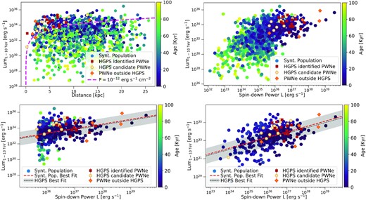
Upper panels: γ-ray luminosity in the 1–10 TeV band (L1–10 TeV) versus source distance (left-hand panel) and pulsar spin-down power (right-hand panel). The entire synthetic population is represented together with the HGPS PWNe (the symbols are specified in the plot legend). The dashed pink curve in the upper left-hand panel is the H. E. S. S. detection threshold flux. Bottom panels: PWNe representation in the L1–10 TeV- |$\dot{E}$| for two different selections of the synthetic population, namely: sources with |$\dot{E}$| > 5 × 1035 erg s−1 (left-hand panel); sources with age <25 kyr (right-hand panel). In both cases, we show the best-fitting relation between the γ-ray luminosity and spin-down power as found in the H. E. S. S. data (black dashed line with standard deviation represented as a shaded grey area) and as determined on our selected population (red dashed line). In both cases, we found an excellent agreement with the best fit to the H. E. S. S. data.
In the other three panels of Fig. 5, we show the TeV luminosity as function of the pulsar spin-down power. Again, we notice that the detected sources represent only the most powerful (L(t) ≳ 5 × 1035 erg s−1) and TeV brightest ones of the entire population. The possible existence of a correlation between the TeV luminosity and the pulsar spin-down power, in analogy to what observed in the X-rays, was investigated by Kargaltsev et al. (2013), who found no clear evidence for such a correlation. On the other hand, the analysis of the wider Fermi energy band (0.1–100 GeV), including also less luminous and less energetic systems than those considered by Kargaltsev et al. (2013), indicates a linear dependence of the γ-ray luminosity on the spin-down power: |$L_\gamma \propto \dot{E}$| (Abdo et al. 2013). More recently, the analysis of the most updated H. E. S. S. data (Abdalla et al. 2018b) suggested indeed a possible correlation between the TeV luminosity and the pulsar power but with a flatter dependence than in the Fermi band: |$L_{1-10\ \rm {TeV}}\propto \dot{E}^{(0.59\pm 0.21)}$|. From the analysis of our population, we surprisingly find a correlation more similar to what deduced from the Fermi analysis than from the H. E. S. S. one. We in fact obtain a slightly super-linear trend: |$L_{1-10\ \rm {TeV}}\sim \dot{E}^{(1.13\pm 0.06)}$|. This might indicate that the submerged part of the non-detected PWNe actually dominates the relation between the emitted γ-ray luminosity and the pulsar spin-down power. It is interesting to notice that a trend similar to that found in the H. E. S. S. data can be retrieved with an appropriate selection of the population. If we consider only sources with |$\dot{E} \gt 5 \times 10^{35}$| erg s−1, we get |$L_{1-10\rm {TeV}}\sim \dot{E}^{(0. 59\pm 0.11)}$|. In the same way, considering only systems younger than 25 kyr, we find |$L_{1-10\rm {TeV}}\sim \dot{E}^{(0.59\pm 0.06)}$|. The direct comparison of these two selections with the trend extracted from the H. E. S. S. data is shown in the lower panels of the same Fig. 5. This exercise clearly shows that the sensitivity of the observations introduces a bias in determining the L1−10 TeV-|$\dot{E}$| relation. At the same time, it shows that our PWNe population well represents the observed ones in the L1−10 TeV-|$\dot{E}$| plane, as long as proper cuts are adopted.
In Fig. 6, we compare the total number of sources with γ-ray flux above 0.1 TeV (plot on the left) and 1.0 TeV (plot on the right), with fluxes expressed in Crab units (CU). To compare with available observations, we limit our analysis to the Galactic plane, with |GLAT| < 2° and GLON < 70°∪GLON > 270°. The synthetic population perfectly reproduces the PWNe (and PWNe + composite) data down to 10−2 CU in both cases. Beyond that value, we see that the observational curves flatten due to the loss of instrumental sensitivity, and below that flux any comparison is meaningless. We also notice that the synthetic population accounts very well for the unidentified sources with higher fluxes, possibly meaning that some of them are in fact unidentified PWNe, as one might also guess from considerations related to the total number of expected PWNe in the Galaxy. In contrast, the unidentified population is not reproduced (by a factor of ∼2) in the range 2 × 10⁻² − 10−1 CU by the synthetic PWNe population. This might be an indication of a different nature of the sources contributing in this energy range (TeV haloes?), or alternatively a problem with our model, due to the oversimplifications introduced.
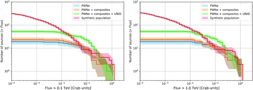
Logarithmic plot of the number of sources emitting in a specific flux range: >0.1 TeV (left-hand panel) and >1 TeV (right-hand panel). The synthetic population (in red) is directly compared with the firmly identified PWNe (in blue), PWNe in a composite SNR (in orange), and the sum of these two with the known unidentified sources (in green). The lighter coloured areas represent the errors of each curve.
We have evaluated the impact on the total TeV flux of our description of relic systems, with particular reference to the assumption that, once escaped, pulsars can never re-enter the PWN bubble, no matter the value of VPSR. These systems represent |$\sim 13{{\ \rm per\ cent}}$| of the overall PWN population at 100 kyr. To assess how their modelling affects our results, we evaluated how the expected TeV flux changes by subtracting from our PWN population all relics whose parent pulsar had escaped before t′; computing the average TeV spectrum of the remaining population; and replacing the contribution of all subtracted relics with this average spectrum. For the time t′, we assumed 100 kyr (corresponding to replacing all relics), 70 kyr and 50 kyr. We found that corresponding flux increases by 11 per cent, 6 per cent, and 4 per cent.This means that, even if relic systems are poorly described from the dynamical point of view, their contribution is such that the global γ-ray emission is affected only by a maximum error of a few per cent.
In Fig. 7, we show the γ-ray efficiency in the 1–10 TeV energy range, |$\epsilon _\gamma =L_\gamma /\dot{E}$|, as a function of the characteristic pulsar age τc (panel on the left) and of the pulsar displacement (panel on the right), comparing with the same quantities as obtained from observations. Information on the source ages is also included with a colour code. Conversely to X-ray efficiency (namely |$L_X/\dot{E}$|) that traces the most recent evolution of the source, the γ-ray efficiency traces the emission along the history of the source; thus, values larger than unity are not unexpected.
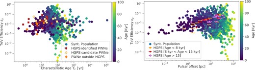
Left-hand panel: Evolution of the TeV efficiency |$\epsilon _\gamma =L_\gamma /\dot{E}$| with the pulsar characteristic age τc, considering the 1–10 TeV range for the γ-ray luminosity. Right-hand panel: Variation of the γ-ray efficiency as a function of the pulsar offset for different age groups (shown in different colours).
On the other hand, those systems would be the oldest, with the largest displacements and extensions. As a result, we can expect that a sizeable fraction of the high γ-ray efficiency systems would not be detected. Having access to the entire population without observational biases, here we can confirm that higher efficiencies at γ-rays are characteristic of objects older than 8 kyr; an efficiency higher than unity is found only for ages >25 kyr and mostly for large pulsar offsets. The occurrence of systems with ϵγ ≳ 1 can be easily interpreted recalling that ϵγ is the ratio between the current values of γ-ray luminosity and pulsar spin-down power, but the former is the result of the entire injection history (as already pointed out by Abdalla et al. 2018b). In any case, we see that only a relatively small number of evolved systems show an efficiency ϵγ ≳ 0.1.
In Fig. 8, we show the PWN distribution as a function of luminosity in different energy ranges and compare our synthetic population (grey) with the number of sources above the detection threshold of existing and upcoming facilities. In the upper panel, we consider sources with luminosities in the range 1–10 TeV and report both the sources that H. E. S. S. can detect (red) and those detected (orange, including also PWN candidates and those marked as outside HGPS), in addition to sources (blue) above the CTA threshold (Remy et al. 2021). One can see that a very large number of sources is expected at Lγ < 1032 erg s−1, and tens of undetected sources with luminosity above the H. E. S. S. threshold are also expected. The reason for this can be understood from comparison with Fig. 5, from which we see that most of these will be at distances >15 kpc, older than 40 kyr and characterized by a residual spin-down luminosity lower than 1035 erg s−1, which makes their identification in the TeV sky extremely challenging. This discrepancy will possibly much reduce with the advent of CTA for which the number of sources above threshold increases by a factor of ∼3 (560 versus 200).
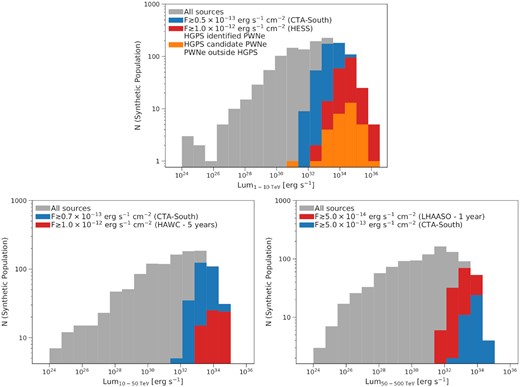
Total number of synthetic PWNe per luminosity beam in different γ-ray luminosity ranges (grey) and number of detectable sources by current and upcoming γ-ray instruments. Upper panel: sources above the H. E. S. S. threshold (red) are compared with the actual detected ones (orange) and with those above the estimated CTA threshold (from Remy et al. 2021, blue) for the 1–10 TeV range. Bottom left-hand panel: expected detections by HAWC (red) and CTA (blue) in the 10–50 TeV range, with detection thresholds estimated from Abeysekara et al. (2013) and Remy et al. (2021), respectively. Bottom right-hand panel: LHAASO (red) versus CTA (blue) in the 50–500 TeV range, with the LHAASO detection threshold estimated from Vernetto (2016).
In the lower panels of Fig. 8, we compare our synthetic population in the 10–50 TeV range (left) with the expected sources detectable by HAWC (red) and CTA (blue), and in the 50–500 TeV range (right) with LHAASO (red) and CTA (blue).
Finally, we think it appropriate to briefly discuss the distribution of sources in the different evolutionary phases at the end of our simulation and compare the results with available data. To date, we know about 20 sources in the free-expansion phase (see e.g. Torres et al. 2014a, Zhu et al. 2018), while only a very limited number of objects have been confirmed to be in a reverberation stage, namely showing direct evidence of the interaction between the PWN and the SNR reverse shock, as observed, e.g. in Vela X (Blondin et al. 2001), Boomerang (Kothes, Reich & Uyanıker 2006), and the Snail (Ma et al. 2016).
In our synthetic population, at the end of the simulated time, we find the sources distributed as follows:
|$\sim 11{{\ \rm per\ cent}}$| of the population (132 sources) is in the free-expansion phase; among these, 103 sources are above the H. E. S. S. threshold flux (27 in the visibility range L > 5 × 1035 erg s−1; F > 10−12 erg s−1 cm−2 discussed in Fig. 5 – about |$2.2{{\ \rm per\ cent}}$| of the population);
|$\sim 76{{\ \rm per\ cent}}$| of the sources have entered the reverberation phase (948 sources); among these, 236 are in the H. E. S. S. detectability range (94 in the visibility region – |$\sim 7.5{{\ \rm per\ cent}}$| of total);
|$\sim 13{{\ \rm per\ cent}}$| of the sources are relic (174 sources); only four of these are above the detection threshold (three in the visibility range – |$\sim 0.2{{\ \rm per\ cent}}$| of total).
As expected, the majority of the sources are middle-aged and hence are in – or have passed through – the reverberation phase. How these numbers compare with the catalogue of observed TeV sources will be discussed in the following section.
5 CONCLUSIONS
Being PWNe the most numerous sources expected to be detected in future γ-ray observations, the problem of how to correctly account for their contribution to the overall γ-ray emission is extremely topical. In this paper, we proposed a physically motivated model of the Galactic PWNe population responsible for the γ-ray emission, taking into account the available observational constraints from known sources. A noticeable difference with respect to previous results is in the pulsar population that we have assumed: we found that in fact the PWN population in the Galaxy is best reproduced when assuming the properties of the powering pulsars as deduced from the γ-ray-emitting pulsar population, rather than from the entire radio pulsar population. This is due to the fact that γ-ray pulsars are representative of a younger population, including the only objects that can indeed power PWNe. The PWNe population was constructed by associating each pulsar of the synthetic population to a core-collapse SNR, using a Monte Carlo method. The entire population was then evolved for 105 yr with a modified one-zone model that incorporates an approximate but reliable recipe to properly account for, both in terms of dynamics and spectral evolution, the complex transition between the free-expansion phase and the late stages, through the so-called reverberation phase. During reverberation, each PWN might experience a sequence of compressions and re-expansions (depending on its energetics and on the properties of the parent SNR), which can modify the spectral properties at the late stages. This phase had not received much attention in the past, since it requires in principle a complex treatment to follow the dynamical evolution of each single source. None the less, it cannot be ignored when the purpose is the modelling of late time γ-ray emission, since this will very significantly depend on the past injection history.
Here, we adopted a simplified but physically motivated model, which was proven to provide a good description of the reverberation phase, based on the results of a large number of HD simulations. In particular, our model takes care of the problem of the artificial over-compression introduced by standard one-zone models that impose the thin-shell approximation also during reverberation. We compare the properties of the evolved population with available data (mainly from the HGPS) and find a very good agreement, especially when considering the intrinsic biases introduced by observational limits. Our simulated population counts around 200 sources above the H. E. S. S. flux detection threshold of ∼10−12 erg s−1 cm−2. These reduce to 124 when considering also the limit on the pulsar luminosity of L ≳ 5 × 1035 erg s−1 discussed in Fig. 5. To date, the second TeVcat catalogue reports a total of 38 TeV sources marked as PWNe or haloes, plus ∼70 unidentified sources, for a total of ∼110 sources. The HGPS found 14 firmly identified PWNe plus ∼45 unidentified sources for a total of ∼60 TeV sources possibly associated with PWNe. Then, around 1/3 of the synthetic population above the H. E. S. S. flux detection threshold can be considered as detected, even if the largest part of the sources has not been identified. The discrepancy between the theoretically expected sources above threshold and the number of TeV detected sources decreases if we consider the visibility limit: of the 124 sources in this region, 1/2 have been detected. The reasons why around |${{\ \rm 50\ per\ cent}}$| of the sources are still missed can be manifold: lack of spatial coverage of present instruments; source confusion and ensuing difficulty of identification; and too large angular extension of the sources.
The situation will change dramatically with CTA, whose detection threshold is expected to be lower by at least one order of magnitude (Remy et al. 2021): the number of theoretically detectable sources will increase to ∼560. Even considering the same factor of 1/3 between revealed and expected sources – likely an underestimate, given that CTA will also have an improved spatial coverage of the sky – this means that around 200 PWNe should be detected in the first CTA Galactic Plane Survey.
ACKNOWLEDGEMENTS
EA, NB, RB, BO, and LZ acknowledge financial support from the Italian Space Agency (ASI) and National Institute for Astrophysics (INAF) under the agreements ASI–INAF n.2017-14-H.0 and from INAF under grants ‘PRIN SKA-CTA’ and ‘Sostegno alla ricerca scientifica main streams dell’INAF’, Presidential Decree 43/2018. EA, RB, and BO also acknowledge support from the INAF grant ‘PRIN-INAF 2019’, LZ from the ASI/INAF grant I/037/12/0. This research made use of gamma-cat, an open data collection and source catalogue for γ-ray astronomy. This research made use also of the following python packages: matplotlib (Hunter 2007), numpy (van der Walt, Colbert & Varoquaux 2011), and astropy (Astropy Collaboration 2018).
DATA AVAILABILITY
The data underlying this article will be shared on reasonable request to the corresponding author.
Footnotes
REFERENCES
APPENDIX A: TRANSITION FROM FREE-EXPANSION TO REVERBERATION PHASE
APPENDIX B: INPUT PARAMETERS FOR THE SIMULATION
In Table B1, we summarize the parameters and relative distribution used as initial condition for the simulation of the PWNe population.
Summary of the input parameters used to generate the PWNe population. Values for the ISM density and IR background photon fields are not listed here since they depend on the position of each source in the Galaxy.
| Parameter | Distribution | Values |
|---|---|---|
| PSRs population parameters | ||
| Braking index | Constant | n = 3 |
| Magnetic field | Lognormal | 〈log10(B/G)〉 = 12.65; |$\, \, \sigma _{\log _{10}B} = 0.55$| |
| Initial spin periods | Equation (1) | 〈P0〉 = 50 ms; |$\, \, \sigma _{P_0} = 50$| ms; (truncated at 10 ms) |
| Kick velocity | Double-sided exponential | 〈v3D〉 = 380 km s−1 |
| SNRs population parameters | ||
| CC SNR masses | Normal | 〈Mej〉 = 13M⊙; |$\sigma _{M_{\rm ej}}=3M_\odot$|; (truncated at 20M⊙) |
| Particle spectrum at injection | ||
| Break energy | Lognormal | 〈Eb〉 ≃ 0.28 TeV; |$\, \, \sigma _{E_\mathrm{ b}} \simeq 0.12$| TeV |
| Low energy index | Uniform | 1.0 < α1 < 1.7 |
| High energy index | Uniform | 2.0 < α1 < 2.7 |
| Magnetic fraction | Uniform | 0.02 < η < 0.2 |
