


ABSTRACT
We use cloudy photoionization models to predict the flux profiles for optical/infrared (IR) emission lines that trace the footprint of X-ray gas, such as [Fe x] 6375 Å and [Si x] 1.43 |$\mu\mathrm{m}$|. These are subset of coronal lines, from ions with ionization potential greater than or equal to that of O vii, i.e. 138 eV. The footprint lines are formed in gas over the same range in ionization state as the H- and He-like of O and Ne ions, which are also the source of X-ray emission lines. The footprint lines can be detected with optical and IR telescopes, such as the Hubble Space Telescope/STIS and James Webb Space Telescope/NIRSpec, and can potentially be used to measure the kinematics of the extended X-ray emission gas. As a test case, we use the footprints to quantify the properties of the X-ray outflow in the type 1 Seyfert galaxy NGC 4151. To confirm the accuracy of our method, we compare our model predictions to the measured flux from archival STIS spectra and previous ground-based studies, and the results are in good agreement. We also use our X-ray footprint method to predict the mass profile for the X-ray emission-line gas in NGC 4151 and derive a total spatially integrated X-ray mass of |$7.8(\pm 2.1) \times 10^{5}\, {\rm M}_{\odot }$|, in comparison to |$5.4(\pm 1.1) \times 10^{5}\, {\rm M}_{\odot }$| measured from a Chandra X-ray analysis. Our results indicate that high-ionization footprint emission lines in the optical and near-IR can be used to accurately trace the kinematics and physical conditions of active galactic nucleus-ionized, X-ray emission-line gas.
1 INTRODUCTION
1.1 General background
Active galactic nuclei (AGNs) are powered by accretion of matter on to supermassive black holes (SMBHs), with masses ≥106 M⊙. This process of feeding the SMBH creates large amount of electromagnetic radiation from the accretion disc of the black hole, which can accelerate winds, and may produce feedback (e.g. Begelman 2004). These winds, if producing efficient feedback, evacuate the bulge of the host galaxy, quenching star formation, which is believed to produce the well-known relationship between the mass of the SMBH and the mass of the bulge (e.g. Gebhardt et al. 2000).
In order to investigate how effective AGN feedback is in galactic-bulge scales, as required in a star-formation quenching, negative feedback scenario, it is important to quantify the mass-outflows properties and their impact on the host galaxy. The physical properties of the gas, such as mass, mass-outflow rates, and kinetic energy can be estimated by photoionization models (e.g. Crenshaw & Kraemer 2007). These models, combined with emission-line studies, particularly those utilizing high spatial resolution (e.g. Fischer et al. 2017; Revalski et al. 2021; Trindade Falcão et al. 2021a), provide the most accurate method to calculate critical quantities of these winds, such as the masses, velocities, outflow rates, and kinetic energies, as a function of distance from the SMBH. The strength of the AGN-driven winds can be quantified in the form of kinetic luminosity, |$\dot{E}(r) = \frac{1}{2} \dot{M}_{\mathrm{out}} v^2$|, where the mass outflow |$\dot{M}_{\mathrm{out}}(r) = 4\pi rN_{\mathrm{H}}\mu m_{\mathrm{p}}C_{\mathrm{g}}v_{\mathrm{r}}$|, and r is the radial distance from the SMBH, NH is the column density, μ is the mean mass per proton, in this case =1.4, mp is the proton mass, Cg is the global covering factor of the gas, and vr is the radial velocity. Studies for efficient feedback require |$\dot{E}(r) \sim 0.5{-}5{{\ \rm per\ cent}}$| of Lbol, the bolometric luminosity of the AGN radiating at near their Eddington limit (Di Matteo, Springel & Hernquist 2005; Hopkins & Elvis 2010). In addition, the amount of kinetic energy deposited into the host galaxy rises rapidly with the velocity of the gas, since |$\dot{E} \propto v^{3}$|.
Our studies of mass outflow in nearby AGN show that, even though these outflows are very massive and inject considerable amounts of kinetic energy in the bulge of the host galaxy, they do not extend far enough to clear the bulge of gas (Fischer et al. 2018) and also lack the power to do so (Trindade Falcão et al. 2021a), since their |$\dot{E}(r)/L_{\mathrm{bol}}$| ratio does not reach the required 0.5 per cent for efficient feedback. Therefore, these results suggest that winds of optical emission-line gas are not an efficient form of AGN feedback (e.g. Trindade Falcão et al. 2021a). However, these results do not take into account the role of higher ionization gas in this process of AGN feedback, which means that it is possible that X-ray winds are responsible for the dynamic effects we observe in nearby AGN (Trindade Falcão et al. 2021b).
Extended soft X-ray emission, colocated with the [O iii] emission-line gas, was detected by Chandra/Advanced CCD Imaging Spectrometer (ACIS) in nearby Seyfert galaxies (Ogle et al. 2000; Young, Wilson & Shopbell 2001). In addition, Chandra imaging has been used to map the narrow-line region (NLR) X-ray emission in several Seyferts (e.g. Bianchi et al. 2010; Gonzalez-Martin et al. 2010; Wang et al.2011a,b, c; Maksym et al. 2019). By isolating bands dominated by specific emission lines, these authors were able to derive constrains on the structure of the X-ray emission-line regions. Notably, Wang et al. (2011b) and Maksym et al. (2019) suggest that there is evidence for shocks, which indicates interaction of the X-ray with the interstellar medium (ISM) of the host galaxy.
Even though it is possible to obtain data with good spectral resolution with Chandra/High Energy Transmission Grating (HETG) (e.g. Kallman et al. 2014; Kraemer et al. 2020), as well as kinematics and detailed physical insights, it is challenging to obtain detailed spatially resolved information from these data. For instance, in their study of NGC 4151, Kraemer et al. (2020) were not able to get any accurate kinematic profiles from the HETG data, even for such a nearby AGN. Therefore, we have no means to determine what role this high-ionization gas plays in the process of AGN feedback.
Alternatively, a model for X-ray gas, characterized by a logU ≈ 0.01 predicts strong optical and infrared (IR) emission lines (see Section 2), which can be considered as ‘footprints’ of the X-ray wind (e.g. Porquet et al. 1999). Since these footprint lines could be detected using ground-based near-IR telescopes (e.g. Rodríguez-Ardila et al. 2011; Lamperti et al. 2017) or the James Webb Space Telescope (JWST; Satyapal et al. 2021) and Hubble Space Telescope (HST)/Space Telescope Imaging Spectrograph (STIS), it provides an opportunity to accurately constrain the kinematics of the X-ray wind.
1.2 Evidence for X-ray feedback
In our most recent paper (Trindade Falcão et al. 2021b), we analysed the dynamics of mass outflows in the NLR of the QSO2 Mrk 34. We presented evidence for the presence of X-ray winds in the NLR of this QSO2 by performing an analysis based on the kinetic energy density of the [O iii]-emitting gas and the X-ray winds, and also by suggesting that high-velocity gas is being accelerated in situ via entrainment by X-ray winds (for details see Trindade Falcão et al. 2021b).
We also used cloudy photoionization models (Ferland et al. 2017) to calculate the integrated fluxes for some of the X-ray footprints, i.e. [Si x] 1.43 |$\mu\mathrm{m}$| and [Fe X] 6375 Å. Even though our X-ray models provided predictions for the [Fe X] that were consistent with the optical spectra, our parametrization of the physical properties of the X-ray winds were determined indirectly, by its inferred dynamical effects and the distributions of the [O III] gas in the NLR of Mrk 34. Therefore, although we were able to obtain results that were consistent with the X-ray emission detected in the Chandra/ACIS image, this does not present itself as a well-constrained model of the X-ray wind.
Kraemer et al. (2020) analysed Chandra/HETG spectra of the X-ray emission-line gas in NGC 4151. The zero-th order data show extended H- and He-like O and Ne, up to a distance r ∼ 200 pc from the nucleus. They determined that the total mass of the ionized gas is |$\approx\!5.4 (\pm 1.1)\times 10^{5}\, {\rm M}_{\odot }$|. In addition, by assuming the same kinematic profile as that for the [O III] gas, derived from the analysis by Kraemer et al. (2000) of HST/STIS spectra, the peak X-ray mass-outflow rate was ≈1.8 |${\rm M}_{\odot }\, {\rm yr}^{-1}$|, at r ∼ 150 pc. The total mass and mass-outflow rates are similar to those determined using [O III] (Crenshaw et al. 2015), which implies that the X-ray gas is a major outflow component. In addition, the fact that it does not appear to be a drop in mass-outflow rates for distances greater than 100 pc may indicate that the X-ray component has a greater effect on the host galaxy than the optical/ultraviolet (UV) gas and that X-ray winds might be a more efficient mechanism for AGN feedback.
Nevertheless, even though the use of Chandra/HETG to characterize the X-ray outflows in NGC 4151 is an improvement compared to the ACIS imaging data used in Trindade Falcão et al. (2021b) to analyse the X-ray winds in Mrk 34, this analysis can only be used to obtain spatially resolved spectra for the most nearby AGN. Additionally, the use of Chandra/HETG is still not enough to fully characterize the extended emission, since this method does not provide accurate spatially resolved kinematics. For this reason Kraemer et al. (2020) made the assumption that the X-ray gas follows the [O III] kinematics and used the [O III] kinematic profile to track the X-ray gas in NGC 4151. In this study, we address this problem by analysing the X-ray outflows in NGC 4151 using a different methodology.
In this paper, we model the X-ray footprint lines using cloudy photoionization models, which allows us to construct radial-flux profiles for these lines. We then compare our predictions to the results of Kraemer et al. (2020) for NGC 4151. In Section 3, we present our photoionization modelling analysis. In Section 4, we present a comparison between our modelling results and the results of Kraemer et al. (2020). Finally, in Sections 5 and 6, we discuss our results and present our conclusions, respectively.
2 THE STUDY OF OPTICAL/IR X-RAY FOOTPRINT LINES
In order to explore the relation between the footprint lines and the X-ray lines we generate a grid of cloudy models using Mrk 34’s spectral energy distribution (SED) and abundances, as discussed in Trindade Falcão et al. (2021a). Our models consider a range in NH of 1020.5–1023.5, a range in logU of (−1.50)–(1.00), and constant density, as the fractional abundance is not a strong function of density. Fig. 1 shows the cloudy-model predictions for the relative abundance of the Fe, Si, and Ca ions, compared to H- and He-like O and Ne, as a function of the ionization parameter and column density. The fact that these lines are formed in gas over the same range in ionization state indicates that they will be formed in gas that will also be the source of X-ray emission lines, detected in the HETG or XMM–Newton/Reflection Grating Spectrometer spectra.
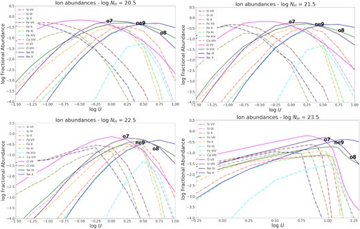
cloudy-model predictions for the fractional abundances of relevant ionization states of Fe and Si and H- and He-like O and Ne, for column densities of logNH = 20.5 (top-left), 21.5 (top-right), 22.5 (bottom-left), and 23.5 (bottom-right). Also, in boldface, we present the logU and fractional abundances for which models predict the maximum fluxes for the X-ray emission-lines O VII -f 22.1 Å, O VIII Ly α, and Ne IX -f 13.7 Å (as discussed in Section 2). As shown here, optical emission lines from ions such as Fe X, Fe XI, Fe XIV, and IR emission lines from ions such as Si X will be formed in the X-ray emitting gas and will act as X-ray ‘footprints’.
It is important to distinguish between coronal lines and footprint lines. Coronal lines are emission lines formed from very highly ionized atoms, and they possess this name because they were first observed in the solar corona (e.g. Mazzalay, Rodriguez-Ardila & Komossa 2010). These lines are collisionally excited forbidden transitions within low-lying levels of highly ionized species with ionization potentials (IPs) ≥100 eV. They have been detected in the optical and IR spectra of all types of Seyfert galaxies (e.g. Seyfert 1943; Nagao, Taniguchi & Murayama 2000; Rodríguez-Ardila et al. 2002; Landt et al. 2015), and represent one of the key gaseous components of the active nucleus. They appear to be approximately equally abundant in type 1 and type 2 AGN (e.g. Rodríguez-Ardila et al. 2011).
On the other hand, we define footprint lines to be a subset of ‘coronal’ lines from ions with IP ≥ 138 eV, i.e. that of O VII, which peak over the same range in ionization parameter as the H- and He-like ions (see Fig. 2). For instance, as shown in Fig. 1 (top-right panel), the fractional abundance for Fe VII, an ionization state which produces a coronal line, peaks at logU ≈ −1.0. Even though its peak ionization parameter is fairly close to that of O VII, the peak flux of the O vii 22.1 Å line is at significantly higher U. Additionally, the peak ionization of O VIII, Ne IX, and Ne X are all at logU > 0. On the other hand, the fractional abundance for Fe X, an ionization state which produces a footprint line, peaks at logU ≈ 0.0, i.e. at the same ionization parameter as the X-ray ions. It is also important to note here that the peak ionic abundance corresponds to the peak flux for collisionally excited lines, like the footprint lines, but not the X-ray lines. These are primarily due to recombination in photoionized plasma, as shown in Fig. 1, hence peak at somewhat higher U than where the ionic abundance is greatest.
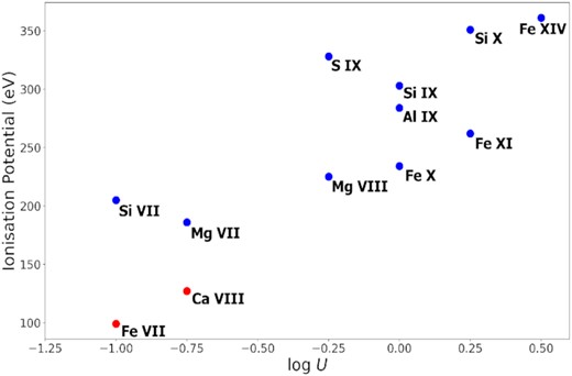
IP of the ions plotted against the ionization parameter where the ion abundances peak. All the models are for logNH=21.5.
In addition, due to its high ionization the gas is optically thin to the ionizing radiation over a large range in column density, which means that our results are not a strong function of the column density of the gas. For example, in Fig. 1 we present the results for the cloudy-model predictions for the fractional abundances of relevant ionization states of Fe and Si and H- and He-like O and Ne, for the following column densities: NH = 1021.5 cm−2 (top-left panel), NH = 1020.5 cm−2 (top-right panel), NH = 1022.5 cm−2 (bottom-left panel), and NH = 1023.5 cm−2 (bottom-right panel). As we can see, the ions from which the footprint lines originate and H- and He-like ions still co-exist over the same range in ionization parameter in a gas with different column densities, which means that our results do not change over a factor of ≳1000 in NH.
Furthermore, we also analyse the effect of different SEDs on the fractional abundances of the relevant ionization states shown in Fig. 1. We use five different SEDs to perform this analysis, specifically, the SED presented by Romano et al. (2004) for the narrow-line Seyfert 1 galaxy Arakelian 564, and the SEDs discussed by Meléndez et al. (2011). Since the choice of SED does not have a significant effect on the accuracy of our method, and to avoid interrupting the flow of the paper, we present these results in Appendix A.
An important point that should be addressed here is the location of [Si VII] and [Mg VII] in Fig. 2. One could think that, since the ionization parameter where their ionic abundances peak is < logU = −0.5, these lines are not footprint lines, even though they satisfy our requirement for their IP, i.e. IP ≥ 138 eV. However, this phenomenon may be due to dielectronic recombination rates (e.g. Kraemer, Ferland & Gabel 2004; Netzer 2004). Specifically, if these rates are too low, the logU values where the ionic abundances peak will also be too low. For example, a shift of 0.25–0.5 dex would be enough to place [Si VII] and [Mg VII] into the ‘footprint’ range.
3 PHOTOIONIZATION MODELLING ANALYSIS
3.1 Photoionization models
For our analysis, we generate photoionization model grids,2 computed using cloudy (version 17.00; Ferland et al. 2017). We assume a continuum source with an SED that can be fitted using a power law of the form Lν∝ν−α. For our study, we adopt the same SED used by Kraemer et al. (2020) in their study on NGC 4151, i.e.
α = 1.0 for 1 × 10⁻⁴ ≤ hν ≤ 13.6 eV;
α = 1.3 for 13.6 eV ≤hν ≤ 500 eV; and
α = 0.5 for 500 eV ≤hν ≤ 30 keV.
In addition, the choice of input parameters, specifically, the radial distances of the emission-line gas with respect to the central source (r), number density (nH), the ionization parameter (U), and column density (NH) of the gas, is that to match the input parameter used by Kraemer et al. (2020), which we will briefly describe.
Kraemer et al. (2020) scaled Q using an average UV flux at 1350 Å observed over the last 7 yr, and computed the value of Q using the assumed SED and a distance of 15 Mpc. They obtained a value of Q = 3 × 1053 photons s−1 and a bolometric luminosity Lbol = 1.4|$\times \ 10^{44}\ {\rm erg\, s^{-1}}$| or 0.03 of the Eddington luminosity.
In addition, the elemental abundances in the NLR of NGC 4151 were initially determined in Kraemer et al. (2000), and based on recent estimates of solar elemental abundances (e.g. Asplund, Grevesse & Sauval 2005), they correspond to roughly 1.4x solar. We assume the same values for this paper, as follows (in logarithm, relative to H, by number): He = −1.00, C = −3.47, N = −3.92, O = −3.17, Ne = −3.96, Na = −5.76, Mg = −4.48, Al = −5.55, Si = −4.51, P = −6.59, S = −4.82, Ar = −5.60, Ca = −5.66, Fe = −4.4, and Ni = −5.78.
We also generate photoionization models that account for internal dust, assuming grain abundances of 50 per cent of those determined for the ISM (e.g. Mathis, Rumpl & Nordsieck 1977), with the depletions from gas phase scaled accordingly (e.g. Snow & Witt 1996), i.e. C = −3.64, O = −3.29, Mg = −4.78, Al = −6.45, Si = −4.81, Ca = −5.96, Fe = −4.70, and Ni = −6.08. These depletions are consistent with more recent studies (e.g. Mehdipour & Costantini 2018). The grain abundance of 50 per cent is the same as that adopted by Kraemer et al. (2000) in their photoionization study of the NLR of NGC 4151.
If the X-ray gas was created from the expansion of [O III] clouds, as discussed in Trindade Falcão et al. (2021b), we expect it to possess internal dust, since the predicted dust temperatures of the X-ray models are too low to be able to destroy the dust grains (e.g. Barvainis 1987). On the other hand, the destruction of dust grains is possible as a result of shocks. If the X-ray gas is entraining clouds of [O III]-emitting gas (Trindade Falcão et al. 2021b) and effectively ‘sweeping’ them up, the shocks that occur during this process could be enough to shatter the dust grains within the gas (e.g. Jones, Tielens & Hollenbach 1997). Our assumption of lower than ISM grain abundance is consistent with this scenario.
3.2 Radial flux distributions
In their study, Kraemer et al. (2020) calculated the emitting area for the X-ray emitting gas. They were able to do this calculation only for Ne IX 13.69 Å and Ne X 12.13 Å, since the loss of soft X-ray sensitivity for ACIS made it hard to accurately measure the O VII 22.1 Å and O VIII 18.97 Å fluxes. To construct the radial-flux profiles associated with each emission line, we redo their analysis, and include in our study other X-ray-line profiles, e.g. O VII 22.1 Å and O VIII 18.97 Å. In addition, in our study, we only generate photoionization models for the medium-ionization component from Kraemer et al. (2020). The reason is that the highest ionization models did not predict significant fluxes for the footprint lines. The complete set of parameters used to generate our models is listed in Table 1.
cloudy model parameters. The models follow the same parameters as the medium-ionization component from Kraemer et al. (2020).
| Distancea | logU | log |$n_{\mathrm{H}}^{a}$| | log |$N_{\mathrm{H}}^{b}$| |
|---|---|---|---|
| cm−3 | cm−2 | ||
| 12 pc | 0.05 | 2.71 | 22.28 |
| 50 pc | −0.17 | 1.69 | 21.88 |
| 100 pc | −0.27 | 1.19 | 21.38 |
| 153 pc | −0.34 | 0.89 | 21.06 |
| 205 pc | −0.38 | 0.68 | 20.81 |
| 257 pc | −0.42 | 0.52 | 20.71 |
| 309 pc | −0.45 | 0.39 | 20.58 |
| 360 pc | −0.47 | 0.28 | 20.27 |
| 412 pc | −0.49 | 0.18 | 20.37 |
| 464 pc | −0.50 | 0.09 | 20.28 |
Note.aBased on density law nH∝r−1.65.
bAssuming δr/r < 1 or δr fixed at 50 pc, where δr is the deprojected width for each extraction bin; for a detailed explanation, see Kraemer et al. (2020).
Using the cloudy predictions for the X-ray footprint lines, and the emitting areas calculated in Kraemer et al. (2020), we also construct radial-flux profiles for the footprint lines, such as [Fe X] 6375 Å and [Si X] 1.43 |$\mu\mathrm{m}$|. Our results are shown in Figs 3 and 3 (Cont.), for the optical/IR lines, and in Fig. 4 for the X-ray lines. It is important to note that our radial-flux profiles show two different sets of models: dust free and 50 per cent dust. The major effect for the dusty models is the depletion of elements on to dust grains. For example, since S and Ne are not depleted from gas phase, the [S X], Ne IX, and Ne X do not show any significant differences, other than a slight increase at the points closest to the AGN. The resulting spatially integrated fluxes for all the footprint and X-ray lines are listed in Table 2.
![Computed radial-flux distributions for X-ray footprint lines [Al IX] 2.04 $\mu\mathrm{m}$, [Ca VIII] 2.32 $\mu\mathrm{m}$, [Fe VII] 6078 Å, [Fe X] 6375 Å, [Fe XI] 7892 Å, [Fe XIV] 5303 Å, [Mg VII] 5.50 $\mu\mathrm{m}$, and [Mg VIII] 3.02 $\mu\mathrm{m}$. The fluxes are obtained using the analysis described in Section 3. The dust-free models are plotted in red and the 0.5 ISM models are plotted in blue. The models assume δr/r < 1 or δr fixed at 50pc, where δr is the deprojected width for each extraction bin. The uncertainties were obtained based on the S/N of the fluxes in the zero-th order image from Kraemer et al. (2020). The positive and negative distances correspond to point SW and NE of the nucleus, respectively.](https://oup.silverchair-cdn.com/oup/backfile/Content_public/Journal/mnras/511/1/10.1093_mnras_stac173/8/m_stac173fig3a.jpeg?Expires=1750312810&Signature=d2zyUcQb5dpPK4xSSDbkcGOVt0~ksKMtzzr-slc3Eq2E1wPSREs1DWu1tZ7R-Pa-h2AXDYY1Cd50yYrODsRHeMu41u-5SHNGhGq~E8pCalz6B54cUyb5LMyTN7LUAoPqRMEN2j3HqucS82f9FERhM4ZhmP2P9DlTR0f~PLNqauSHPBBI6WdQxJckysYTzOZBJunkV~4Khda~-2QWqH4v7AJDmWzS1vbSvMZXJ5a1bdTRrxTws89jQTQY5XCEbJyHyQL~KYayao2bjjJtSMcGclp7saO8AmcyBcSr8-Pgqljy9qGcin3JjfBHyTjAcYtVrCLMPWJzJB3wa2PFrZZY1Q__&Key-Pair-Id=APKAIE5G5CRDK6RD3PGA)
![Computed radial-flux distributions for X-ray footprint lines [Al IX] 2.04 $\mu\mathrm{m}$, [Ca VIII] 2.32 $\mu\mathrm{m}$, [Fe VII] 6078 Å, [Fe X] 6375 Å, [Fe XI] 7892 Å, [Fe XIV] 5303 Å, [Mg VII] 5.50 $\mu\mathrm{m}$, and [Mg VIII] 3.02 $\mu\mathrm{m}$. The fluxes are obtained using the analysis described in Section 3. The dust-free models are plotted in red and the 0.5 ISM models are plotted in blue. The models assume δr/r < 1 or δr fixed at 50pc, where δr is the deprojected width for each extraction bin. The uncertainties were obtained based on the S/N of the fluxes in the zero-th order image from Kraemer et al. (2020). The positive and negative distances correspond to point SW and NE of the nucleus, respectively.](https://oup.silverchair-cdn.com/oup/backfile/Content_public/Journal/mnras/511/1/10.1093_mnras_stac173/8/m_stac173fig3b.jpeg?Expires=1750312810&Signature=wgz0cBpd1SeJlfTRVLLm2GWknHouOcyT42KjohYSF7tcOTf~q7EZBwHSDFh4lHml3B31COQsQ93sL6UiZgs9xqdr1dTbeiRq45hxxjMdCQwXNSWzGr1JUvz4mVgQsHKXp5LC3h-tIjvxsOIpYFrK3CD5NcRAk~aeHXQSh8FhRCt8JFx0A2gj-PrkZgllwBDhCLJoqY9478eYBgzFzXSi2rCeZ~KTSP19mqmK~i7n4DCtX3UB729Ul2Uuz0dQIUgIj9tC9iXmspOd2FX89MZ6zyiGKwOPKrJW7XtpfKL7yFQ49mEyiOgG-ZEdWuY2qsScUPnzVvYdlIJ7vY-gGYiXoQ__&Key-Pair-Id=APKAIE5G5CRDK6RD3PGA)
Computed radial-flux distributions for X-ray footprint lines [Al IX] 2.04 |$\mu\mathrm{m}$|, [Ca VIII] 2.32 |$\mu\mathrm{m}$|, [Fe VII] 6078 Å, [Fe X] 6375 Å, [Fe XI] 7892 Å, [Fe XIV] 5303 Å, [Mg VII] 5.50 |$\mu\mathrm{m}$|, and [Mg VIII] 3.02 |$\mu\mathrm{m}$|. The fluxes are obtained using the analysis described in Section 3. The dust-free models are plotted in red and the 0.5 ISM models are plotted in blue. The models assume δr/r < 1 or δr fixed at 50pc, where δr is the deprojected width for each extraction bin. The uncertainties were obtained based on the S/N of the fluxes in the zero-th order image from Kraemer et al. (2020). The positive and negative distances correspond to point SW and NE of the nucleus, respectively.
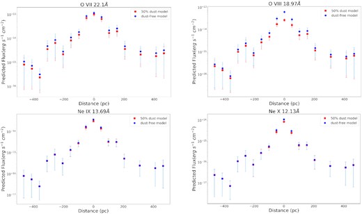
Computed radial-flux distributions for X-ray lines O VII 22.1 Å, O VIII 18.97 Å, Ne IX 13.69 Å, and Ne X 12.13 Å. The fluxes are obtained using the analysis described in Section 3. The dust-free models are plotted in red and the 0.5 ISM models are plotted in blue. The models assume δr/r < 1 or δr fixed at 50pc, where δr is the deprojected width for each extraction bin. The uncertainties were obtained based on the S/N of the fluxes in the zero-th order image from Kraemer et al. (2020).
Predicted spatially integrated fluxes. In boldface are the emission lines that we define as footprint lines, i.e. lines from ions with IP ≥ 138 eV.
| Ion | Wavelength | IP | Peak logU* | Predicted flux dfa | Predicted flux db | Observed flux |
|---|---|---|---|---|---|---|
| (eV) | |$({\rm 10^{-16}\, erg\, s^{-1}\,cm^{-2}})$| | |$({\rm 10^{-16}\, erg\, s^{-1}\,cm^{-2}})$| | |$({\rm 10^{-16}\, erg\, s^{-1}\,cm^{-2}})$| | |||
| [Al IX] | 2.04 |$\mu\mathrm{m}$| | 284 | 0.0 | 51.8 (±4.8) | 6.9 (±0.6) | 23 (±16)c |
| [Ca VIII] | 2.32 |$\mu\mathrm{m}$| | 127 | −0.75 | 3.9 (±0.6) | 5.3 (±0.5) | 151 (±23)c |
| [Fe VII] | 6087Å | 99 | −1.0 | 15.4 (±2.0) | 26.5 (±2.5) | – |
| [Fe X] | 6375Å | 234 | 0.0 | 2360 (±215.0) | 1050 (±96.2) | 1900d |
| [Fe XI] | 7892Å | 262 | 0.25 | 921 (±87.7) | 302 (±27.7) | – |
| [Fe XIV] | 5303 Å | 361 | 0.5 | 130 (±15.6) | 34.0 (±3.9) | <750d |
| [Mg VII] | 5.50 |$\mu\mathrm{m}$| | 186 | −0.75 | 35.2 (±4.2) | 37.1 (±3.4) | – |
| [Mg VIII] | 3.02 |$\mu\mathrm{m}$| | 225 | −0.25 | 251 (±24.8) | 174 (±15.9) | – |
| [S IX] | 1.25 |$\mu\mathrm{m}$| | 328 | −0.25 | 22.0 (±2.2) | 31.1 (±2.9) | 397 (±23)c |
| [Si VII] | 2.48 |$\mu\mathrm{m}$| | 205 | −1.0 | 14.6 (± 1.7) | 16.9 (±1.5) | – |
| [Si IX] | 3.55 |$\mu\mathrm{m}$| | 303 | 0.0 | 319 (±33.0) | 195 (±17.3) | – |
| [Si X] | 1.43 |$\mu\mathrm{m}$| | 351 | 0.25 | 559 (±51.9) | 214 (±19.5) | 377 (±30)c |
| O VII f | 22.1Å | 138 | −0.5 | 3940 (±359.0) | 3230 (±293.0) | 3400(±769)e |
| O VIII α | 18.97Å | 739 | 0.25 | 610 (±146.0) | 880 (±79.5) | 1089(±192)e |
| Ne IX i | 13.69Å | 239 | 0.0 | 851 (±79.4) | 747 (±69.1) | 1041(±96)e |
| Ne X α | 12.13Å | 1195 | 0.75 | **204 (±19.8) | 166 (±15.8) | 480(±48)e |
Notes.aDust-free models.
b50 per cent dust models.
cObserved fluxes from Rodríguez-Ardila et al. (2011).
dObserved fluxes from this study.
eObserved fluxes from Kraemer et al. (2020).
*The values of logU are to the nearest 0.25 dex. All the models are for log NH=21.5.
**Most of the X-ray emission accounted for this line comes from the high-ionization components modelled by Kraemer et al. (2020). However, since these models do not significantly contribute to the footprint-line emission we decide not to include them in this study.
It is important to note that a few of our predicted flux profiles, such as [Ca VIII] and [Fe VII] (see Fig. 3) show a higher predicted flux for the dusty models in the centre bins. This is because the He ii zone is shallower when dust is present, which results in greater recombination into those ionization states. However, the effect is not present for the more distant points, because NH is smaller (see Table 1); hence, the model integrations do not reach the end of the He ii zone (see discussion in Kraemer & Harrington 1986).
4 FOOTPRINTS OF X-RAY OUTFLOWS
4.1 Observational limits on the footprint lines
By analysing the archival STIS long-slit spectra, we are able to obtain the spatial [Fe X] and [O III] distribution in NGC 4151, as shown in Fig. 5. Specifically, since the [Fe X] λ6375 emission line is contaminated by [O i] λ6364, we obtain an intrinsic [Fe X]-brightness profile by subtracting 1/3 of the [O i] λ6300 flux at each point along the slit. In addition, in order to account for the mass of [Fe X]-emitting gas outside of the area sampled by the STIS slit, we use an archival HST/WFPC2 [O III] image of the NLR for the target (Kraemer et al. 2020). We measure the [O III] fluxes in regions of 0|${_{.}^{\prime\prime}}$|5 x 3|${_{.}^{\prime\prime}}$|0, centred at the nucleus, along a position angle of 140○.
![Spatial distribution for [Fe X] (in black) and [O III] (in red) in NGC 4151. The values were obtained from the analysis of the STIS G750L spectrum. The fluxes are per cross-dispersion pixel (0.1 arcsec × 0.05 arcsec).](https://oup.silverchair-cdn.com/oup/backfile/Content_public/Journal/mnras/511/1/10.1093_mnras_stac173/8/m_stac173fig5.jpeg?Expires=1750312810&Signature=ZNlGbvHtakH8WfmxxbVpeV7ztf6ie46CJFjSz5OjswD85VJ3I2Ke1sRLVcZ5facoHcQhR5CLcjekQhPjESbyJvfEwaXQPes9ZxJy4mkBpgKQLF07o9bHzN266sCsFSdwxXwRbW5lmXb-0eFt4fixtK2MLHCVLZfKJfHZgFqanRhT6~wv8MRVWr2yF8rhxwPt4P8jBxLs3jXUWSiAuDq89QwBe32LdHDnvjNzn3aD05-oKodXcrQDlWoxDeBrHfOZ4rH0dCbHSIhBhviH~mUJ9RXn-rAoHVTEnS31RuqSMeNl4m8XkVkmbo8WSh5d-qRqJBt727yOCr6Sc7vH9YAxpw__&Key-Pair-Id=APKAIE5G5CRDK6RD3PGA)
Spatial distribution for [Fe X] (in black) and [O III] (in red) in NGC 4151. The values were obtained from the analysis of the STIS G750L spectrum. The fluxes are per cross-dispersion pixel (0.1 arcsec × 0.05 arcsec).
We then measure the ratio [Fe X]/[O III] inside the STIS slit, which allow us to obtain the full [Fe X]-flux distribution. In Fig. 6, we compare the results of our predicted [Fe X]-flux profiles (both for dust-free models and 50 per cent dust models) and the results of the full [Fe X]-flux distribution (inside and outside the slit). The total spatially integrated [Fe X] flux, i.e. the sum of the fluxes inside and outside the STIS slit, is |$1.9^{+0.6}_{-0.2}\times 10^{-13}\ {\rm erg\,s^{-1}\,cm^{-2}}$|. It is important to note here that the flux profiles show lower fluxes for the negative distances. This is because the observed fluxes are asymmetric around the nucleus, which is not easily seen in Fig. 5, since the slit did not cover the entire NLR.
![A comparison between the results of our predicted radial-flux profiles for the [Fe X]-emitting gas (the blue points represent the dust-free model values and the red points represent the 50 per cent dust model values) and the results of the full [Fe X]-flux distribution (inside and outside the STIS slit). The uncertainties were obtained based on the S/N of the fluxes in the zero-th order image from Kraemer et al. (2020). Additionally, the flux profiles show lower fluxes for the negative distances. This is because the observed fluxes are asymmetric around the nucleus, which is not easily seen in Fig. 5, since the slit did not cover the entire NLR.](https://oup.silverchair-cdn.com/oup/backfile/Content_public/Journal/mnras/511/1/10.1093_mnras_stac173/8/m_stac173fig6.jpeg?Expires=1750312810&Signature=glf0jI60mpiwthAN6z5QErGXpRiQ-G1ZCOopfa3NNWmVmPuJTnFs4rnGX2bvPi2BQ1xqrJzM7zhAC7bep-M41rVdxPOU0cqaLJnJ3l18HXL-ozGsTZ9YFQoBbR9G0tovD40mqUQMYjLHzKdjTVtwlM0EM0VpVy5t08Qb4CTxbhLhVrmYb8RM7w69B~06gJukLVu2U3pBRDGOAU~pWUzF09yg9rrG5gtAMJxzceL3AL2xaxLchwozlt0yKtIoTUWYR1x7bqoXyTh-6SIjyASB~0~q7oUIjKLpGovHBkAjGFZbXjEz-UvCn98tRTT-sJpUxrUPO-~xKY-f1jF2odlZDg__&Key-Pair-Id=APKAIE5G5CRDK6RD3PGA)
A comparison between the results of our predicted radial-flux profiles for the [Fe X]-emitting gas (the blue points represent the dust-free model values and the red points represent the 50 per cent dust model values) and the results of the full [Fe X]-flux distribution (inside and outside the STIS slit). The uncertainties were obtained based on the S/N of the fluxes in the zero-th order image from Kraemer et al. (2020). Additionally, the flux profiles show lower fluxes for the negative distances. This is because the observed fluxes are asymmetric around the nucleus, which is not easily seen in Fig. 5, since the slit did not cover the entire NLR.
In addition, based on the analysis of the STIS long-slit spectra, we are able to calculate an upper limit, integrated over 11 pixels (0.1 arcsec × 0.55 arcsec), for the flux of the [Fe XIV] 5303 Å line <7.5 × 10⁻¹⁴ erg s−1 cm−2, which agrees with our predicted flux of 1.3 × 10⁻¹⁴ erg s−1 cm−2 (see Table 2). Considering that the brightness profile for [Fe XIV] follows the same brightness profile as [Fe X], we calculate an upper limit in the central bin 0.1 arcsec × 0.05 arcsec < 2.6 × 10⁻¹⁴ erg s−1 cm−2, which also agrees with our predicted value of 1.0 × 10⁻¹⁴ erg s−1 cm−2. It is important to note here that the other optical footprint lines are below the detection limit of STIS.
4.2 Predicting the mass of the extended gas
In order to recompute the mass of the extended X-ray gas in NGC 4151 based on our X-ray footprint analysis, we use our predicted [Fe X] radial-flux profile. It is important to note here that the methodology used in this study to estimate the mass of the extended X-ray gas in the target is different from the methodology used by Kraemer et al. (2020). Kraemer et al. (2020) mapped the Ne IX triplet (the resonance line, 13.50 Å; the intercombination line, 13.60 Å; and the forbidden line, 13.73 Å) and Ne X α, instead of [Fe X], and applied the model parameters to fit the zero-th order emission-line profiles of these lines.

Even though our results for the total mass of X-ray-emitting gas are very promising, due to the poor resolution of the STIS grating used for this observation, along with a low S/N, we are not able to obtain any accurate kinematic information for [Fe X]. This means that we cannot compute the outflow rates for NGC 4151, and a comparison to the values for |$\dot{M}$| found by Kraemer et al. (2020), i.e. |$\dot{M}$| = 1.8 M⊙ yr−1, is not possible given the available STIS low-dispersion spectrum.
5 DISCUSSION
In Fig. 8, we present the cloudy-predicted [Fe X]/H β (in red), O VII (22.1 Å)/H β (in blue), and O VII (21.6 Å)/H β (in green) ratios for NGC 4151, for the 50 per cent dust fraction models. It is possible to see that when densities are very high, i.e. ≳108.0 cm−3, the [Fe X]/H β ratio starts to drop, which means that the [Fe X] 6375 Å line starts to become collisionally suppressed. However, the O VII (22.1 Å)/H β ratio also drops with increasing density, hence [Fe X] still tracks the O VII 22.1 Å emission. On the other hand, the O VII 21.6 Å line is not suppressed over this range in density. Therefore, there could be a contribution to the X-ray-emitting gas from denser regions, close to the AGN. However, for NGC 4151, Q ≈ 3 × 1053 photons s−1 (e.g. Kraemer et al. 2020), so gas characterized by logU = 0.0 with densities of ≈109 cm−3 would lie at r ≈ 2.8 × 1016 cm from the central SMBH, which is just at the outer edge of the broad-line region (BLR; about 10 light-days, e.g. Bentz et al. 2013). The fact that our predicted values for the mass of X-ray-emitting gas in NGC 4151 agree very well with the measured values by Kraemer et al. (2020; see Fig. 7) tells us that the contribution from X-ray gas that is located in the BLR of this AGN is negligible. This result is consistent with the findings of Crenshaw & Kraemer (2007), which shows that the mass outflows from the dense inner region of the AGN do not contribute significantly to the total gas in the NLR of NGC 4151, and the gas located in this region, i.e. in the NLR, is likely accelerated in situ.
![Predicted [Fe X]/H β (in red), O VII -f/H β (in blue), and O VII -r/H β (in green) ratios for NGC 4151. The model assumptions are: abundances (1.4x solar), SED from Kraemer et al. (2020), constant column density NH = 10$^{21.5}\, {\rm cm^{-2}}$, and ionization parameter logU = 0.0.](https://oup.silverchair-cdn.com/oup/backfile/Content_public/Journal/mnras/511/1/10.1093_mnras_stac173/8/m_stac173fig8.jpeg?Expires=1750312810&Signature=1912RO~aUrqOmf~c9FeAWDg~9u-4-s~ozL03s~zLiOEcNjjxkBXiETVXWw3GIh02bsbA5-m~bI7LgkPBBwXeU1he0eXfxdaqXIIgqRvkD~Ky1JgG1psKGXlcAPfJntVyA7MFCyJexu~gFxnihlz24YJxtcAGA4k6InaQsg4FahHK6cVwbCRDQXjUQHVKAvfgBYS-OdvUw02MPqxN0FABefxwHy-vruLk8BZnzXkodRfoRJ~0eXImu89l3XqiDcPyQ92orqoy8juAfc1kZ2uHpi4oGbfU9G95AdwR2su3XW7u5xIRtraSmLSYGva2XWyvmDnlWvceUgdg6dx869BrMg__&Key-Pair-Id=APKAIE5G5CRDK6RD3PGA)
Predicted [Fe X]/H β (in red), O VII -f/H β (in blue), and O VII -r/H β (in green) ratios for NGC 4151. The model assumptions are: abundances (1.4x solar), SED from Kraemer et al. (2020), constant column density NH = 10|$^{21.5}\, {\rm cm^{-2}}$|, and ionization parameter logU = 0.0.
As discussed in Section 3, internal dust can have a significant effect on how we interpret our results. As shown in Figs 3 and 3 (Cont.), the presence of dust within the outflowing gas can have a more pronounced effect in some lines, e.g. [Fe X] 6375 Å, compared to others, e.g. [S IX] 1.25 |$\mu\mathrm{m}$|. The fact that the [S IX] fluxes do not seem to be heavily affected by the presence of dust within the gas, as shown in Fig. 3 (Cont.), tells us that this line might be a good choice of footprint line when the percentage of dust within the gas is unknown (but see below). On the other hand, for lines like [Fe X] 6375 Å and [Mg VIII] 3.02 |$\mu\mathrm{m}$|, it is important to have a good estimate of the amount of dust present in the gas, since their fluxes are strongly affected by depletion of these element on to dust grains. For instance, if one uses only the [Fe X] 6375 Å line to predict the emission of X-ray gas, but underestimates the amount of dust within the gas, the estimated X-ray mass could be overestimated, since the dusty models predict lower fluxes, as shown in Fig. 3.
In addition, Rodríguez-Ardila et al. (2011) measured the fluxes of IR footprint lines for NGC 4151 in their study of near-IR coronal line spectrum of nearby AGN. As shown in Table 2, our predicted fluxes for [Al IX] 2.04 |$\mu\mathrm{m}$| and [Si X] 1.43 |$\mu\mathrm{m}$| agree well with the results of Rodríguez-Ardila et al. (2011). The underprediction of [Ca VIII] 2.32 |$\mu\mathrm{m}$| is consistent with the fact that Ca VIII peaks at much lower ionization than our X-ray models (see Fig. 1). Regarding the discrepancy between our measured flux for the [S IX] 1.25 |$\mu\mathrm{m}$| and the observed flux from Rodríguez-Ardila et al. (2011), we believe that our underpredicted value could be due to collision strength of this transition (e.g. Zhang & Sampson 2002), or due to an unmodelled process, such as photoexcitation/photofluorescence.
It is important to note that in this study, we use [Fe X] as a tracer for X-ray outflows based on the characteristics of NGC 4151, i.e. the fact that this target is not a very powerful AGN. For AGN with more highly ionized gas in their NLR, other lines would be a better choice, such as [Si X] and [Fe XIV], as shown in Fig. 1. For instance, based on our predicted flux and observed flux for [Fe XIV] 5303 Å (see Table 2), there is not a large amount of [Fe XIV] in NGC 4151 and this is because there is only a small amount of high-ionization gas in the NLR of this target. For more powerful targets, e.g. quasars, the use of [Fe XIV] as a tracer might be preferable, since these objects are more luminous and powerful than NGC 4151.
6 CONCLUSIONS
Based on our analysis derived from cloudy photoionization models, we present a new method that can be used to model X-ray outflows. Our conclusions are as follows:
There are ions that peak over the same range in ionization parameter as the H- and He-like ions and can produce detectable optical/IR emission lines, which we call ‘footprint lines’. These lines can be detected and spatially resolved, e.g. via HST or JWST observations and, therefore, can be used to accurately measure the kinematics and the dynamics of the extended X-ray gas. For instance, footprint lines such as [Al IX], [Si VII], [Si IX], and [Si X] can be observed with JWST, and, for Near InfraRed Spectrograph (NIRSpec) IFU, where most of the footprint lines are, the spectral resolving power R∼100, 500, 1000s (depending on the mode) corresponds to a velocity resolution of <∼100–300 km s−1, which will allow us to obtain good kinematic information on the targets and, subsequently, be able to fully characterize the X-ray outflows.
We show that the models based on Chandra data from Kraemer et al. (2020) predict strong footprint lines, which is consistent with the HST data. We also develop flux profiles to characterize such lines.
By analysing the STIS long-slit spectrum and the [O III] image for NGC 4151, we are able to derive the measured flux profile for [Fe X] 6375 Å within similar extraction bins.
We compare our model predictions to the observed flux profile for [Fe X] obtained from the analysis of the STIS G750L spectrum. Our values are in very good agreement with the measured values, which confirm the reliability of our approach. We also compare our model predictions for the IR lines to the observed fluxes from Rodríguez-Ardila et al. (2011), which show very good agreement for the [Al IX] 2.04 |$\mu\mathrm{m}$| and [Si X] 1.43 |$\mu\mathrm{m}$| (see Section 5 for caveat on predicted IR footprint lines).
We confirm our methodology by determining the mass of X-ray gas using our models predictions and the observed flux profile for the [Fe X]. As shown in Fig. 7, our values are in very good agreement with the values found by Kraemer et al. (2020), which confirms that our method can accurately produce mass profiles for the X-ray gas.
Even though we are able to produce accurate mass profiles for the X-ray gas using our method of ‘footprint lines’, we are not able to get accurate kinematic information for these lines from the STIS data. The poor resolution of the STIS G750L grating, combined with low S/N, does not allow us to obtain the necessary kinematic information to compute the values for outflow rates of this target. It would be interesting to obtain observations with higher spectral resolution for NGC 4151, which would allow us to compute the predicted mass-outflow rates and again test our proposed methodology. Another possibility is to apply this method on other AGN, such as NGC 1068, for which the combination of X-ray spectra and medium-resolution STIS long-slit spectra exist. In addition, it is important to note that, even though we do not need the kinematic profiles derived from X-ray observations to apply our method, we would still need X-ray spectra to compare with photoionization models in order to fully characterize the ionization structure of these outflows.
ACKNOWLEDGEMENTS
The material is based upon work supported by NASA under award number 80GSFC21M0002. Basic research at the Naval Research Laboratory is funded by 6.1 base funding.
This research has made use of the NASA/IPAC Extragalactic Database (NED), which is operated by the Jet Propulsion Laboratory, California Institute of Technology, under contract with the National Aeronautics and Space Administration. This paper used the photoionization code cloudy, which can be obtained from http://www.nublado.org. We thank Gary Ferland and associates, for the maintenance and development of cloudy.
DATA AVAILABILITY
This research is based on observations made with the NASA/ESA Hubble Space Telescope, and data underlying this article are available from the Hubble Legacy Archive, which is a collaboration between the Space Telescope Science Institute (STScI/NASA), the Space Telescope European Coordinating Facility (ST-ECF/ESAC/ESA), and the Canadian Astronomy Data Centre (CADC/NRC/CSA).
Footnotes
|$U= \frac{Q}{4\pi n_{\mathrm{ H}}r^{2}c}$|, where, nH is the hydrogen number density, r is the distance to the ionizing source, c is the speed of light, and the ionizing luminosity, |$Q = \int _{\nu _{0}}^{\infty } L_{\mathrm{v}} \, \mathrm{ d}\nu$|, where hν0 = 13.6 eV.
The SEDs modelled by Meléndez et al. (2011) are characterized by α = 0.5 for hν < 13.6 eV, α = 1.0−2.5 between 13.6 < hν < 1 keV, and α = 0.8 for hν > 1 keV.
REFERENCES
APPENDIX A: SED analysis
As noted in Section 2, we also explore the effect of different SEDs on the fractional abundances of relevant ionization states of Fe and Si and H- and He-like O and Ne. To perform this analysis we use the SED present by Romano et al. (2004) and the range of power-law SEDs presented by Meléndez et al. (2011). The different SEDs used and our results are shown in Fig. A1.

Top-left panel: Representation of the five SEDs used in our analysis. Top-right panel: cloudy-model predictions for the fractional abundances of relevant ionization states of Fe and Si and H- and He-like O and Ne. The model assumptions are: abundances (1.4x solar), SED from Romano et al. (2004), and constant column density NH = 1021.5 cm−2 (e.g. Kraemer et al. 2020; Trindade Falcão et al. 2021b). As shown here, optical emission lines from ions such as Fe X, Fe XI, and Fe XIV, and IR emission lines from ions such as Si X will be formed in the X-ray-emitting gas and will act as X-ray ‘footprints’. Bottom-left panel: Same as top-right panel, but with an SED from Meléndez et al. (2011) with α = 1.0 between 13.6 < hν < 1 keV. Bottom-right panel: Same as top-right panel, but with an SED from Meléndez et al. (2011) with α = 2.5 between 13.6 < hν < 1 keV. The results shown in the top-right, bottom-left, and bottom-right panels can be compared to our results using the Mrk 34 SED (Fig. 1) and the results from the NGC 4151 analysis (see Table 2).
In Fig. A1, we show the results of our analysis for α = 1.0 between 13.6 <hν < 1 keV, and α = 2.5 between 13.6 <hν < 1 keV, i.e. the lower and upper values of the range modelled by Meléndez et al. (2011).3 As we can see in Fig. A1, the ions from which the footprint lines originate and H- and He-like ions still co-exist over the same range in ionization parameter, even when considering sources with various SEDs. Note that for α = 2.5 between 13.6 <hν < 1 keV, there are relatively fewer EUV and X-ray photons; therefore, the fractional abundances peak at higher ionization parameter than for the harder SEDs, as shown in the bottom-right panel in Fig. A1. However, it is possible to see that the optical/IR footprint lines still co-exist over the same range in ionization parameter as the X-ray lines, which confirms the accuracy of our method, even for very soft SEDs.
