


ABSTRACT
We use data from the first-year observations of the DES collaboration to measure the galaxy angular power spectrum (APS), and search for its BAO feature. We test our methodology in a sample of 1800 DES Y1-like mock catalogues. We use the pseudo-Cℓ method to estimate the APS and the mock catalogues to estimate its covariance matrix. We use templates to model the measured spectra and estimate template parameters firstly from the Cℓ’s of the mocks using two different methods, a maximum likelihood estimator and a Markov Chain Monte Carlo, finding consistent results with a good reduced χ2. Robustness tests are performed to estimate the impact of different choices of settings used in our analysis. Finally, we apply our method to a galaxy sample constructed from DES Y1 data specifically for LSS studies. This catalogue comprises galaxies within an effective area of 1318 deg2 and 0.6 < z < 1.0. We find that the DES Y1 data favour a model with BAO at the |$2.6 \sigma$| C.L. However, the goodness of fit is somewhat poor, with χ2/(d.o.f.) = 1.49. We identify a possible cause showing that using a theoretical covariance matrix obtained from Cℓ’s that are better adjusted to data results in an improved value of χ2/(dof) = 1.36 which is similar to the value obtained with the real-space analysis. Our results correspond to a distance measurement of DA(zeff = 0.81)/rd = 10.65 ± 0.49, consistent with the main DES BAO findings. This is a companion paper to the main DES BAO article showing the details of the harmonic space analysis.
1 INTRODUCTION
The large-scale distribution of galaxies carries information about the cosmological model that best describes our Universe (e.g. Dodelson 2003; Lyth & Liddle 2009). After the great success of maps of the cosmic microwave background (CMB) in providing cosmological information, large galaxy surveys have become one of the major contributors to our understanding of gravity and the ingredients that make up the cosmos. They provide evidence for the consistency of our description for the evolution of the Universe from the early CMB epoch to present times.
The distribution of galaxies in the Universe carries cosmological information that was imprinted from the era when baryons and photons were tightly coupled. The so-called baryon acoustic oscillation (BAO) feature results from processes that occur up to the baryon drag epoch, and are sensitive in particular to the sound horizon rs at decoupling.
It is possible to quantify the distribution of galaxies by measuring its 2-point correlation function. One can measure the three-dimensional 2-point galaxy correlation function either in real space or measure its Fourier transform, the power spectrum, in harmonic space. In principle both quantities carry the same information, but in practice they may have different sensitivities to the estimation of cosmological parameters due to, among other effects, different covariance matrices, different response to systematic effects, etc. For instance, Gaussian covariance matrices for the power spectrum are diagonal in the full-sky case, whereas for the spatial correlation function significant correlations are expected. Hence performing measurements in both real and Fourier space serves as a consistency check, and may also provide complementary information to tame some of the observational issues.
In galaxy surveys where redshifts are not precisely measured, as is the case with photometric redshifts (photo-z), one actually considers the projected galaxy distribution into redshift bins. In this case what is measured is the angular correlation function in real space [ACF, denoted by w(θ)] and/or the angular power spectrum in harmonic space (APS, denoted by Cℓ in the following).
The APS is studied in this work, which uses data from the first year (Y1) of observations from the Dark Energy Survey (DES; Flaugher 2005), a large photometric survey in five bands that is planned to cover 5000 deg2 of the sky in a 5-yr campaign. The DES uses the Dark Energy Camera (DECam; Flaugher et al. 2015), a 570-Megapixel camera mounted on the 4-m Blanco telescope at the Cerro Tololo Inter-American Observatory, Chile and is currently in its fifth year of data acquisition. The DECam received its first light in 2012 September, followed by a science verification (SV) period covering an area of approximately 250 deg2. Measurements of the ACF and the impact of systematic errors in the SV data were reported in Crocce et al. (2016). More recently, cosmological results from combined clustering and weak lensing measurements in the DES Y1 data have been presented (Abbott et al. 2017a).
The BAO feature in the 2-point galaxy correlation function has been observed in several surveys. A few examples are the 2-degree Field Galaxy Redshift Survey (2dFGRS) (Percival et al. 2001; Cole et al. 2005), the Sloan Digital Sky Survey (SDSS) I, II, III, and IV (Eisenstein et al. 2005; Padmanabhan et al. 2012; Anderson et al. 2014a; Ross et al. 2015; Alam et al. 2017; Ata et al. 2018), and the WiggleZ survey (Blake et al. 2011). In particular, the BAO scale was measured in SDSS photometric samples using the ACF (Sawangwit et al. 2011; Carnero et al. 2012; de Simoni et al. 2013) and the APS (Blake et al. 2007; Seo et al. 2012).
In this work we use a template-based method to study the BAO feature in the angular power spectra from the DES Y1 data. We describe our method and test it on realistic survey mocks. These mocks were also used to measure the covariance matrix of the Cℓ’s. The covariance matrix was then used to find the likelihood corresponding to the template adopted to model the data. We estimate the significance of the detection of the BAO feature for a baseline template using two independent methods: a maximum likelihood estimator (MLE) and a Markov Chain Monte Carlo (MCMC) method. We also present the reduced χ2 values for the mocks to demonstrate the goodness of fit. We explore the robustness of our baseline model to the estimation of parameters testing different choices of settings and assumptions in the analysis. After the validation of our methodology we apply it to Y1 data with the intent to search for BAO features. We find that the DES Y1 data favour a model with BAO wiggles at the |$2.6\sigma$| confidence level with a best-fitting shift parameter of α = 1.023 ± 0.047 with a somewhat large value of χ2/(dof) = 1.49. We investigate this issue substituting the covariance matrix obtained from the mocks by a Gaussian theoretical covariance matrix taking into account the Y1 mask with input Cℓ’s that are better adjusted to data obtaining an improved value of χ2/(dof) = 1.36 which is similar to the value obtained with the real-space analysis.
This paper is part of a series related to the detection of the BAO features in Y1 data. It relies on the construction of a catalogue suitable for the study of clustering of galaxies, especially concerning the BAO feature (Crocce et al. 2017), the mock catalogues used to validate the analysis and results (Avila et al. 2017) and the computation of galaxy photo-zs (Gaztanaga et al. in preparation). Other papers detail methods to study the BAO feature in configuration space with the angular correlation function w(θ) (Chan et al. 2018), and using the comoving transverse separation (Ross et al. 2017), while this work details the use of the APS. The joint results applied to the Y1 data are described in the BAO main paper (Abbott et al. 2017b).
This paper is organized as follows. We start by describing the theoretical modelling of the APS in Section 2, including the template used to study the BAO feature. In Section 3, we describe the DES Y1 galaxy catalogue constructed for BAO studies, focussing on the redshift binning, pixelization, and masking. The 1800 mock catalogues used for the verification of our measurements, for the covariance matrix estimation and for testing our parameter estimation from the template method are briefly presented in Section 4. In Section 5, the measurement of the APS using the pixelized maps is described. The methodology we adopt is tested on the mocks in Section 6 where we also study the impact of different choices of templates and settings on the parameter estimation as robustness checks. Having validated our methodology, we apply it for Y1 data in Section 7 where we concentrate on finding BAO features in the APS. Finally, in Section 8 we present our conclusions.
2 THEORY
In this section we review basic concepts used for the theoretical modelling throughout the paper.
2.1 Angular power spectrum and theoretical covariance matrix
We decompose |${\bf x}=\chi (z)\hat{\bf n}$| where |$\hat{\bf n}$| is the angular direction and χ(z) is the comoving angular-diameter distance at redshift z. Since we only consider flat-universe cosmologies, χ(z) is simply the comoving radial distance to redshift z.
The analytical expression we actually use to estimate the theoretical covariance is more realistic, as it is tied to the pseudo-Cℓ estimator (see Section 5) and corrects for binning and mask effects (Efstathiou 2004). Interestingly, we find that the above approximation multiplied by a boost factor agrees well with the full covariance expression and with the covariance estimated from mock catalogues in the range of ℓ explored in this work (see Section 6.2). The angular mask weights enter in the computation of the mask-corrected Gaussian covariance matrix. However, the weights do not enter in the covariance matrix derived from the Halogen mocks.
2.2 Cℓ template
Our goal is to extract from mocks and from DES Y1 observations the scale associated with the BAO feature, namely the angular distance scale DA(z). In order to be as insensitive as possible to non-linear effects such as bias and redshift space distortions, we will use a template method (Seo et al. 2012; Anderson et al. 2014b; Gil-Marín et al. 2016; Ross et al. 2017; Ata et al. 2018; Chan et al. 2018)
We will test this parametrization with the mocks below and show that it results in biases below |$1 {{\ \rm per\ cent}}$| for the parameter estimation. We study the impact of other templates as robustness tests in Section 6.
3 DES Y1 GALAXY CATALOGUE
3.1 Catalogue
The catalogue for LSS analyses using DES Y1 data was created from the so-called Y1 Gold catalogue (Drlica-Wagner et al. 2018) which in turn was built from the data reduction performed by the Dark Energy Survey Data Management (DESDM) system on DECam images. The LSS sample selection is based on colour, magnitude, and redshift cuts designed to provide an optimal balance between the density of objects and the photometric redshift uncertainty for z > 0.6, minimizing the forecasted BAO error (Crocce et al. 2017). We will use the LSS catalogue with photometric redshifts obtained with a multi-object fitting (MOF) photometry (Drlica-Wagner et al. 2018) and the directional neighbourhood fitting (DNF) algorithm (De Vicente, Sánchez & Sevilla-Noarbe 2016). After proper masking described in Crocce et al. (2017) the catalogue has approximately 1.3 million galaxies in an area of 1317 deg2.
We divide the catalogue into four tomographic photo-z bins with width Δzphot = 0.1 in the range 0.6 < zphot < 1.0. In Fig. 1, we show the redshift distribution for each bin obtained by stacking a Monte Carlo sampled value of the photo-z from the estimated probability distribution function for each object. The bins are defined using a point-estimate of the photo-z given by the maximum likelihood redshift produced by DNF.
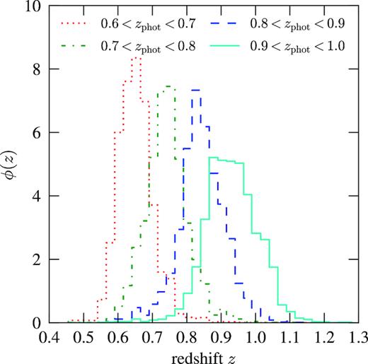
Redshift selection function ϕ(z) ∝ dN/dz in the four photo-z bins considered in this work.
Stacking the estimated redshift PDFs of individual sources is not guaranteed to reproduce the redshift distribution of a sample. Fortunately, Crocce et al. (2017) validate the photo-z distribution for the BAO sample and Chan et al. (2018) investigate the impact on the estimated BAO angular scale from systematic errors in the mean and variance of photo-z distributions, finding that the expected systematic uncertainty of the mean induces a systematic error of |$0.8{{\ \rm per\ cent}}$| on the recovered angular BAO scale, which is small compared to our statistical errors. Hence the systematic errors in the redshift distribution parametrized by a shift parameter can be safely neglected.
The LSS catalogue also comes with a correction for the three main systematic dependencies found on observational quantities: local stellar density, mean i-band PSF (FWHM) and detection limit (g-band depth). These corrections are encapsulated in a weight factor wsys for each object, which is applied to reduce these dependencies. See Crocce et al. (2017) for details.
3.2 Pixelized map generation
These maps generated for each redshift bin are used to measure the APS as explained in Section 5.
4 DES MOCK SIMULATIONS
In addition to the DES Y1 galaxy catalogue, we use a set of 1800 galaxy mock simulations, especially made for studies of large-scale structure in DES, including the present BAO analysis (Avila et al. 2017).
These mocks serve a dual purpose in our study. First, we use them to test our codes for estimating Cℓ’s, covariances and the BAO feature extraction in a DES-like survey. Secondly, we make direct use of the covariance matrices estimated from them in the BAO analysis of the DES Y1 data.
These simulations match all aspects of the DES Y1 data, including its footprint, abundance and clustering of galaxies and redshift distribution. One starts with halo catalogues that are constructed with the HALOGEN method (Avila et al. 2015), such that they satisfy halo-mass functions and bias appropriately from N-body simulations. Next, galaxies are assigned to these haloes according to a hybrid halo occupation distribution (HOD)/halo abundance matching (HAM) prescription. The methodology is much faster than using full N-body simulations and allows for the construction of thousands of simulations. These mock catalogues were constructed using the MICE Grand Challenge N-body simulations (Crocce et al. 2010; Crocce et al. 2015; Fosalba et al. 2015a,b), with cosmological parameters close but not equal to those of the Planck mission. We refer the reader to Avila et al. (2017) for details of the construction of these DES galaxy mocks.
5 ANGULAR POWER SPECTRUM MEASUREMENT IN CUT SKY
When performing full-sky estimations, we compute the coefficients aℓm from the pixelized density contrast maps using the anafast routine within healpix.
We use two independent codes to measure Cℓ’s via the pseudo-Cℓ method without shot-noise subtraction. The first code is our own implementation of the pseudo-Cℓ method in python. The second is the publicly available code namaster,1 which is implemented in C. We compared the Cℓ’s estimated from the two codes when applied to a single DES mock simulation. The two codes agree at better than 5 per cent for all ℓ values considered here, and better than 1 per cent for ℓ > 100, indicating our measurements are robust. All results presented in the remainder of the paper will make use only of the namaster code.
We consider in our default analysis multipoles in the range 30 < ℓ < 330, corresponding roughly to the angular scales used in the w(θ) analysis (Chan et al. 2018), and we then bin using a bin width of Δℓ = 15 in order to make the reduced covariance matrix more diagonal and amenable to algebraic manipulations. Effects of different ranges and binnings will be studied as robustness tests in Section 6.4.
6 TESTS OF METHODOLOGY ON MOCKS
We now apply our full methodology on the 1800 DES Y1 HALOGEN mock simulations with known cosmology and perform robustness tests to estimate the impact of changing our default settings on parameter estimation.
6.1 Measurements of the APS
In Fig. 2, we show the results of our Cℓ measurements in the four photo-z bins for the 1800 mocks together with the mean of the mocks. We also show theoretical predictions from Cℓ’s computed with a linear matter spectrum at the same cosmology as the mocks. In each photo-z bin, we multiply the theoretical matter Cℓ’s by a galaxy bias factor squared determined by Avila et al. (2017) and add a shot-noise determined by the number density of Y1 galaxies in that photo-z bin.
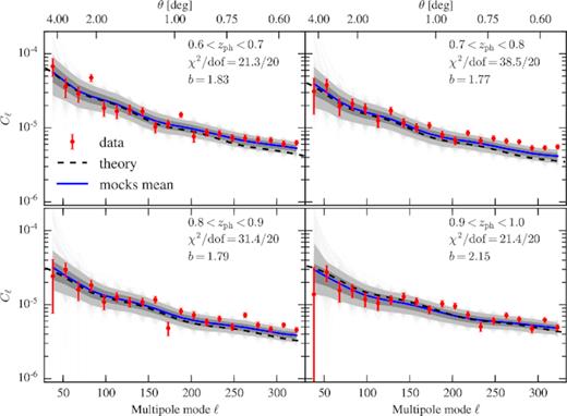
Measurements of Cℓ in four photo-z bins for the 1800 mocks (grey lines) and the Y1 data (red circles). Dashed line shows the theoretical prediction from a linear spectrum with MICE cosmology multiplied by a bias factor (shown in the panels) and including shot-noise and shaded regions show |$68{{\ \rm per\ cent}}$| and |$95{{\ \rm per\ cent}}$| C.L. from mocks measurements. The blue line is the average of the mocks. The χ2 values show reasonable agreement between average measurements of the mocks and measurements on data.
The measured Cℓ’s from the mocks are in good agreement with the theoretical prediction. However, when compared to data there is some discrepancy in the second and third redshift bins, reflected in the somewhat high value of χ2 = 1.92 and 1.57, respectively. In these bins the Cℓ’s from data exceed the ones from the mocks at large ℓ’s. We will discuss some consequences of this behaviour below.
6.2 Covariance matrix
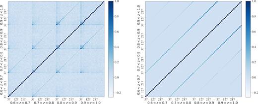
Cℓ’s correlation matrix for the four photo-z bins. Left: measured from the 1800 mock simulations mimicking the DES Y1 data. Right: Theoretical estimation computed at the mock cosmology, and accounting for binning and mask effects.
In Fig. 4, we compare the diagonal errors of the Cℓ’s estimated from the mock simulations and the Gaussian prediction of the fiducial cosmology using two approximations: the naive fsky approximation equation (13) and the prediction of the covariance matrix of the pseudo-Cℓ estimator (Efstathiou 2004; Brown, Castro & Taylor 2005). We find good agreement between the errors coming from the simulation covariance matrix and from the pseudo-Cℓ estimator. However, for the fsky approximation we find that a ‘boost factor’ of 1.35 is necessary to match the measured errors. This was also the case for a similar analysis in SDSS (Ho et al. 2012).
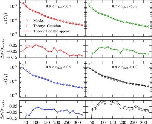
Comparison of the Cℓ’s diagonal errors in four photo-z bins. For each bin, the top panel shows the standard deviation estimated from the 1800 DES mock simulations (open circles) the Gaussian prediction on the fiducial cosmology (solid lines) after rescaled by an empirical boost factor of 1.35 and the Gaussian prediction from the pseudo-Cℓ method (open triangles). The bottom panels show the relative differences with respect to the mocks standard deviation.
We will use the full covariance matrix estimated from the mocks. It is well known that statistical noise on the estimation of the covariance matrix from mock realizations translates into a bias on its inverse, the precision matrix, which is the actual fundamental piece on the likelihood estimation. We included this correction factor in our analysis (Hartlap, Simon & Schneider 2007; Dodelson & Schneider 2013; Percival et al. 2014). Given the number of mocks used, we have checked that the correction factor for the precision matrix is always less than 5 per cent, having no impact on the recovered value of α.
6.3 Parameter estimation
We use two independent methods for the parameter estimation: an MCMC implemented with emcee (Foreman-Mackey et al. 2013) and an MLE with analytical least square fit of the nuisance parameters (Cowan 1998). We used our default BAO template described in Section 2.2 with the covariance matrix estimated from the mocks. We performed a joint fit for the four photo-z bins with 17 parameters in our default template.
In Fig. 5, we show the distribution of α values resulting from fits of our Cℓ measurements in four photo-z bins for the 1800 mocks. The remaining 16 parameters are marginalized over for the MCMC analysis and fixed to the values that maximize the likelihood for the MLE analysis as described in Chan et al. (2018). For the MLE method we find the best fit analytically over the 12 parameters A0, A1, A2 in each redshift bin and numerically over the 4 B0’s requiring B0 > 0 for each value of α, following Chan et al. (2018).
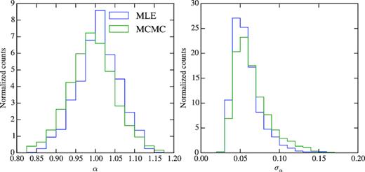
Left: distribution of the recovered α for the detected mocks. Right: distribution of the estimated error on α. Results from different methods are presented.
For the MCMC we used the flat priors α ∈ [0.8, 1.2], A1 ∈ [ − 800, 800] × 1010, A2 ∈ [ − 50, 50] × 106, A3 ∈ [ − 200, 200] × 103, and B0 ∈ (0, 6].
We exclude outliers defined as mocks whose 1σ values for α lie outside the range 0.8 < α < 1.2 (see Chan et al. 2018) using the MLE method. For our fiducial analysis |$86.4 {{\ \rm per\ cent}}$| of the mocks are kept.
Since our fiducial model has the same cosmology as the mocks we expect to find α = 1. In fact we find that the mean value in the mocks is |$\bar{\alpha }=1.006$| for MLE and |$\bar{\alpha }=0.992$| for MCMC. Therefore both our methods recover α with a bias at the sub per cent level.
In Fig. 6 we show the results from the MCMC chains when fitting the BAO template to the averaged Cℓ measured in the mock simulations for our fiducial template. In this case, we find for the shift parameter α = 0.988 ± 0.060 and it can be seen that it does not show strong correlations with the nuisance parameters. In fact, the nuisance parameters are poorly constrained, having broad distributions. The best-fitting values for B0 and A0 are found to be roughly consistent with the squared bias and the shot-noise in each bin, respectively. For the MLE method we find α = 1.009 ± 0.056 from a fit to the average of the mocks.
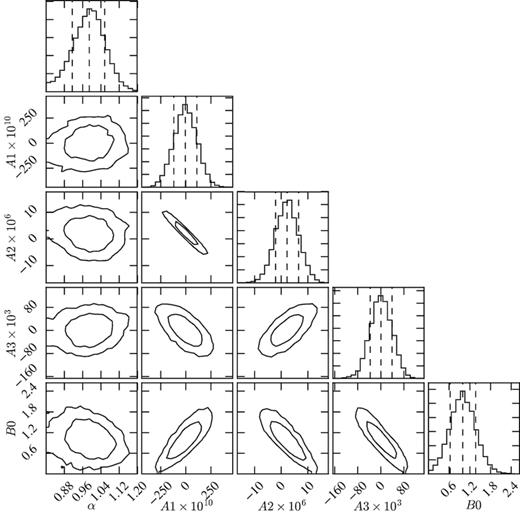
Fit results for α and template parameters B0, A0, A1, and A2 in the first photo-z bin for a BAO template fitted to the average of the 1800 DES mock simulations. The plots for the parameters in other bins are similar.
In Fig. 7, we show Cℓ’s measured in four photo-z bins for the DES mock simulations. The errors are computed from the mock covariance matrix. The solid line displays the best-fitting theoretical prediction using the BAO template described in Section 2.2. We see that our BAO template is able to accurately capture the behaviour of the Cℓ’s from the mocks.
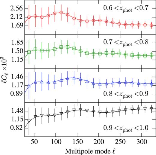
Measured Cℓ’s from DES mock simulations in four photo-z bins. The points show the average Cℓ’s from 1800 simulations and the error bars represent the diagonal of the covariance matrix of these measurements. The line shows a theoretical prediction estimated at the simulation cosmology and best-fitting template parameters.
The compatibility between the two independent methods (MCMC and MLE) is shown in Fig. 8 where we plot the normalized likelihood for the α parameter determined from the average of the mocks for both methods.
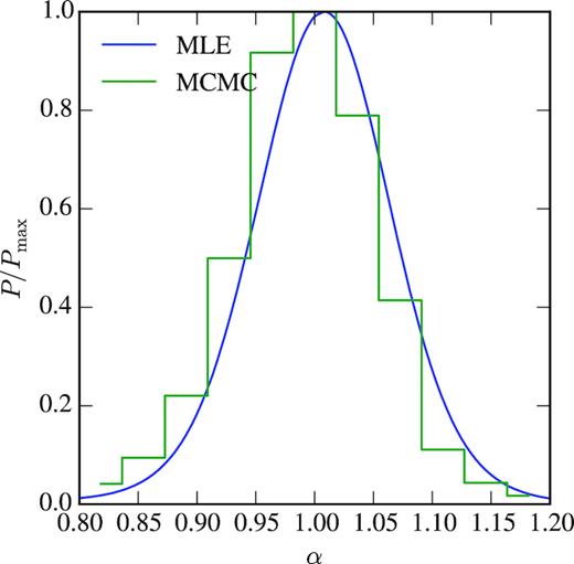
Normalized likelihoods from the MLE (solid line) and MCMC (histogram) methods for the α parameter determined from the average of the mock Cℓ’s.
In Fig. 9, we show the distribution of χ2 for the 1800 mocks demonstrating the good fit of our template. Also shown in the plot as a dashed line is the χ2 obtained from the data using the covariance matrix estimated from the mocks (discussed in Section 7).
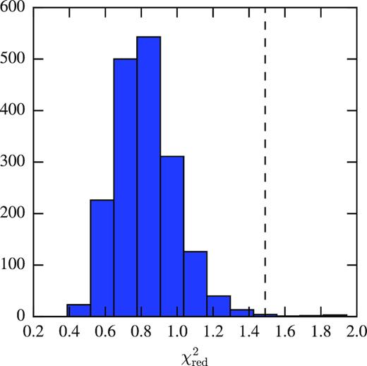
Distribution of the reduced χ2 values for the 1800 mocks. The dashed line shows the value of χ2 obtained from the data using the covariance matrix estimated from the mocks (Section 7).
We estimate the significance of recovering α (or detecting the BAO feature) by measuring the difference in χ2 as a function of α between a model with no BAO feature (a no-wiggle model), which is independent of α, and our BAO template. In Fig. 10, we show |$\Delta \chi ^2=\chi ^2(\alpha)-\chi ^2_{\rm min}$| for fits of the average Cℓ’s from the mocks as a function of the α parameter. The best-fitting value is αmin = 1.009. From Fig. 10, we see that for the average of the mocks a BAO signal would be detected at 2.3σ with respect to a no-wiggle model.
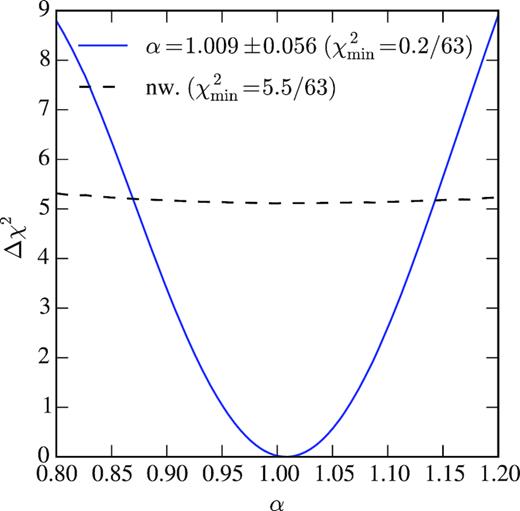
|$\Delta \chi ^2=\chi ^2(\alpha) - \chi ^2_{\rm min}$| as a function of α for the BAO template fitted on the mean of mocks. For each value of α we subtract from χ2 the value of |$\chi ^2_{\rm min}=\chi ^2(\alpha _{\mathrm{ min}})$|. Dashed line is the approximately constant χ2 for the non-wiggle template subtracted from the minimum of the template.
We will use the methods described in this section to study the BAO signal in Y1 data. But before doing so, we use the mocks to perform some robustness tests related to choices made in our analysis.
6.4 Robustness tests
For our default analysis above, a number of choices were made: the binning of harmonics in Δℓ = 15, adopting ℓmin = 30 and ℓmax = 330, and the fiducial template used. We recall that we are including linear RSD in the modelling and we are using the full covariance matrix with redshift bin cross-correlations. We have examined the impact on the parameter estimation and on the fraction of detection of the mocks (the fraction of mocks remaining when excluding outliers) for some other choices. A summary of some of our tests is shown in Table 1, for choices of binning and range of ℓ as well as Cℓ templates. We conclude that our choice of template gives an unbiased result for α at the per cent level and a reasonable detection fraction. Although different choices produce small changes in the fits, they do not affect the BAO detection significantly, showing that our analysis is robust.
Summary of the robustness tests performed on the 1800 mocks using MLE. We show the average values of α and its 1σ standard deviation for all the mocks, the standard deviation of α obtained only for the detected mocks Sα, and the fraction of detected mocks. The fiducial case we adopt has a template A0 + A1ℓ + A2ℓ−2 and Δℓ = 15, 30 < ℓ < 330 shown in boldface.
| Case | 〈α〉 | 〈σ〉 | Sα | f(Ndet) | Mean of mocks |
|---|---|---|---|---|---|
| Δℓ = 15, 30 < ℓ < 330: | |||||
| A0 + A1ℓ + A2ℓ−1 | 1.003 | 0.051 | 0.058 | 0.752 | |$1.008 \pm 0.056\,$| |
| |$\mathbf {A_0+A_1 \ell +A_2 \ell ^{-2}}$| | |$\mathbf {1.007}$| | |$\mathbf {0.058}$| | |$\mathbf {0.053}$| | |$\mathbf {0.864}$| | |$\mathbf {1.009 \pm 0.056}\,$| |
| A0 + A1ℓ + A2ℓ2 | 1.011 | 0.056 | 0.055 | 0.851 | |$1.013 \pm 0.056\,$| |
| Δℓ = 20, 40 < ℓ < 300: | |||||
| A0 + A1ℓ + A2ℓ−1 | 1.003 | 0.051 | 0.060 | 0.734 | |$1.006 \pm 0.058\,$| |
| A0 + A1ℓ + A2ℓ−2 | 1.006 | 0.059 | 0.056 | 0.812 | |$1.006 \pm 0.058\,$| |
| A0 + A1ℓ + A2ℓ2 | 1.009 | 0.057 | 0.057 | 0.790 | |$1.012 \pm 0.057\,$| |
| Δℓ = 15, 45 < ℓ < 330: | |||||
| A0 + A1ℓ + A2ℓ−1 | 1.004 | 0.050 | 0.059 | 0.736 | |$1.009 \pm 0.056\,$| |
| A0 + A1ℓ + A2ℓ−2 | 1.007 | 0.057 | 0.054 | 0.841 | |$1.009 \pm 0.056\,$| |
| A0 + A1ℓ + A2ℓ2 | 1.011 | 0.056 | 0.055 | 0.839 | |$1.013 \pm 0.056\,$| |
| Δℓ = 20, 40 < ℓ < 320: | |||||
| A0 + A1ℓ + A2ℓ−1 | 1.004 | 0.050 | 0.060 | 0.731 | |$1.008 \pm 0.056\,$| |
| A0 + A1ℓ + A2ℓ−2 | 1.007 | 0.058 | 0.055 | 0.833 | |$1.008 \pm 0.057\,$| |
| A0 + A1ℓ + A2ℓ2 | 1.011 | 0.056 | 0.057 | 0.831 | |$1.014 \pm 0.057\,$| |
In addition to the tests in Table 1, we have also investigated other choices made. These included (i) using the Limber approximation (Limber 1953) instead of the full integral calculation in equations (9) and (11), (ii) exclusion of linear RSD effects, i.e. using equation (10) instead of equation (11), (iii) exclusion of cross-correlations between photo-z bins in the covariance matrix, (iv) use of the theoretical covariance instead of the covariance measured in mocks, and (v) inclusion of the non-linear matter power spectrum in the Cℓ modelling. All these tests led to very similar results as the fiducial analysis for α.
Notice that (i) and (ii) affect large scales while (v) affects only small scales. Meanwhile we expect (iii) and (iv) to have small effects given that redshift cross-correlations are small for our photo-z bin size and the theoretical covariance matches that measured in the mocks quite well (see Section 6.2). Our Cℓ template has enough flexibility to account for these effects in case they are either included or neglected. Indeed we find that the best-fitting template parameters change significantly between one case and another, but the best fit for α and the BAO detection significance remain nearly the same.
7 BAO IN DES Y1 DATA
We now apply the methods described and tested above to study the BAO feature in the APS in the DES Y1 data. In Fig. 11, we show Cℓ’s measured in four photo-z bins for the DES Y1 data. The errors are computed from the variance of the 1800 mock simulations. The solid line displays the best-fitting theoretical prediction using the BAO template described in Section 2.
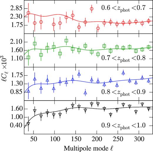
Measured Cℓ’s from DES Y1 data in four photo-z bins. The errors represent the diagonal of the covariance of 1800 mock simulations. The line shows our best fits from the fiducial analysis.
In Fig. 12, we show the |$\Delta \chi ^2=\chi ^2(\alpha)-\chi ^2_{\rm min}$| of the fits as a function of α for the DES Y1 data from the MLE described above and also used in Chan et al. (2018). We find α = 1.023 ± 0.047 with |$\chi ^2_{\rm min}/{\rm dof}=93.7/63=1.49$|. This somewhat large value of χ2 seems to indicate that the covariance matrix obtained from the mocks may underestimate the errors. We will discuss this possibility below.
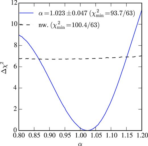
Δχ2 as a function of α for the DES Y1 galaxy data, when fitted to a BAO templates (solid blue curve) and to a no-wiggle template (dashed black curve).
The small deviation of α from unity can be traced to the fact that the template cosmology has been fixed to reflect that of the mock simulations (to be consistent with the fact that we also use the covariance from the mock simulations). The mocks have a cosmology slightly different from e.g. the Planck cosmology, and the latter has been shown to be consistent with clustering measurements of the DES Y1 data (Abbott et al. 2017a; Gruen et al. 2018). A difference of a few per cent in α from unity is expected and is also found in a similar analysis in configuration space (Abbott et al. 2017b; Chan et al. 2018). However, this difference is not statistically significant given the error. We have repeated our analysis with the covariance matrix re-calculated at the best-fitting cosmology, and we have not found significant changes in our results, which was also the case for Abbott et al. (2017a).
Finally, we also show the difference in χ2 from our best-fitting template and a no-wiggle model. Assuming Gaussian statistics for the likelihood, we find that the APS measured from DES Y1 data finds the BAO feature at a significance of |$2.6 \sigma$| level with respect to a no-wiggle template.
As for the robustness tests on mock data, for the analysis on the data, we further consider the impact of the systematic weights and the cross signal in the covariance matrix as explained below.
We compute a χ2 for the corrections induced by including the associated weights, |$\chi ^2_{\rm sys} = \Delta C_\ell ^{\rm T} \Psi \Delta C_\ell$|, where |$\Delta C_\ell =(C_\ell ^{\rm weighted}-C_\ell)$| and Ψ the precision matrix. The square root of this quantity offers an upper bound for the ‘number of σ’s’ that weights could bias the determination of any model parameter. For the fiducial scale-cuts of the analysis we find |$\chi ^{2 (i)}_{\rm sys} = 0.62, 0.24. 0.29$|, and 0.95, respectively for each photo-z bin i individually and |$\chi ^2_{\rm sys} = 0.43$|. This implies that by considering each photo-z individually, an extreme case for the last bin appears in which if weights are not properly considered, results can be shifted by almost one σ. However, by combining information on all bins, the impact is reduced to 0.66σ. We also perform the analysis without correcting by the weights, obtaining a fit α = 1.019 ± 0.058 with goodness of fit of χ2 = 98/63, with no apparent implication on the error estimation and goodness of fit, but leaving a shift in the dilation parameter of 0.085σ, well below the upper bound from |$\chi ^2_{\rm sys}$|. This can be understood as an indication of the BAO feature not being easily reproducible by contaminants and insensitive to its corrections in agreement with configuration space analysis of Crocce et al. (2017).
When excluding the cross signal in the covariance matrix used in the analysis of the data we obtain α = 1.045 ± 0.049 with a χ2 = 93/63, showing a negligible change with respect to our fiducial analysis which includes the cross signal in the covariance matrix (notice that the data vectors used in the analysis are only the auto power spectra).
In order to address the issue of the large value of χ2 obtained above we study the changes that arise from using a theoretical covariance matrix better adjusted to the data. We use a HaloFit power spectrum prediction (Takahashi et al. 2012) with MICE cosmological parameters, supplemented by the galaxy bias and shot-noise measured on the Halogen mocks and taking into account linear redshift space distortions. In the resulting APS, we added a term proportional to ℓ with a coefficient that was allowed to vary for each redshift bin. These four coefficients were fitted using the DES Y1 data. This theoretical Cℓ was then input into namaster to compute a new Gaussian covariance matrix that accounts for the Y1 mask and the binning in ℓ. When this new covariance matrix is used the minimum χ2 is indeed reduced to |$\chi ^2_{\rm min}/{\rm dof}=85.8/63=1.36$| without a significant change in the estimated value of α, which is found to be α = 1.039 ± 0.053 in this case.
In Fig. 13, we show the result of the significance using this new theoretical covariance matrix. The value of α changed by a third of the standard deviation and the error increased by |$13{{\ \rm per\ cent}}$|. Although the changes are small they point to the uncertainties inherent in this analysis.
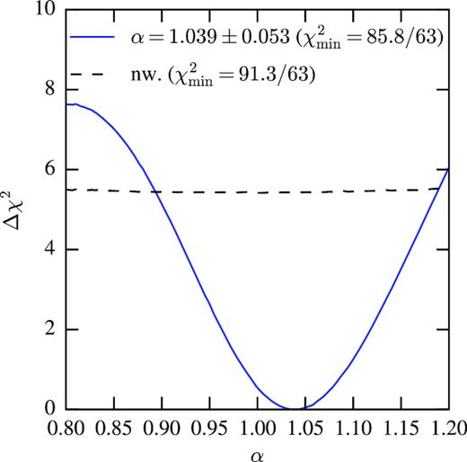
Δχ2 as a function of α for the DES Y1 galaxy data, when fitted using a new theoretical covariance matrix to a BAO template (solid blue curve) and to a no-wiggle template (dashed black curve).
8 CONCLUSIONS
The DES is on its way to produce the largest survey to date, projected to map 300 million galaxies using photometric techniques in an area of 5000 deg2 up to a redshift z ≈ 1.3. The Y1 data have been recently analysed resulting in a key paper combining three correlations: weak gravitational lensing, galaxy clustering, and their cross-correlation or galaxy–galaxy lensing (Abbott et al. 2017a). Several papers dealing with the essential developments that led to the key paper were also produced (Avila et al. 2017; Cawthon et al. 2017; Davis et al. 2017; Gatti et al. 2017; Krause et al. 2017; Drlica-Wagner et al. 2018; Hoyle et al. 2018)
The work presented here is part of a series of papers mentioned in the introduction dedicated to searching specifically for the BAO feature in Y1 data. Here we concentrated on the detection of the BAO feature in the APS. The main goal of this paper was to provide a harmonic-space counterpart to the analysis made in configuration space (Abbott et al. 2017b). We did not attempt to fully optimize the catalogue and strategy for mitigating systematic errors in our harmonic-space analysis. Instead we simply used the catalogue and systematic tools that were optimized for the configuration-space analysis. It is possible that systematic errors absent or unimportant for the analysis in configuration space may be relevant in some range of ℓ′s in harmonic space, and we hope to investigate this in further detail on DES Y3 data. However, our final results were all comparable to those of configuration space, which indicates that further optimization would have a small effect in our results.
We developed a methodology based on template-fitting and tested it on realistic DES Y1 galaxy mocks. First we tested two independent codes for pseudo-Cℓ estimators and found agreement between codes to better than 1 per cent in nearly all scales of interest. We then measured the APS in four photo-z bins for 1800 mock catalogues, checking their consistency with theoretical expectations. We measured the covariance matrix from the mocks and compared it with a theoretical prediction, finding again good agreement. We then used two independent methods, an MLE and an MCMC analysis to estimate the shift parameter for the average of the mocks and found the two methods to be compatible. Comparing the values of χ2 for our BAO template to a no-wiggle model we find a |$2.3 \sigma$| signal for BAO in the mocks.
Several choices were made for our fiducial analysis and we performed a number of robustness tests to assess their impact on the results. We find that our results on the mocks were not significantly sensitive to changing the binning Δℓ from 10 to 20, changing the smallest scales of our analysis from ℓmax = 300 to ℓmax = 330, neglecting the redshift cross-covariance, using the Limber approximation, neglecting linear RSD’s, including a non-linear matter power spectrum and modifying the Cℓ template used.
We then applied the fiducial analysis to measure the APS of a galaxy sample obtained from DES Y1 data also split into four photo-z bins up to z = 1 (Crocce et al. 2017). We obtain a best-fitting α = 1.023 ± 0.047. This corresponds to a measurement of the ratio of the angular diameter distance to the effective redshift of our sample (zeff = 0.81) and the BAO physical scale rd of DA(zeff = 0.81)/rd = 10.65 ± 0.49. Comparing to the best-fitting no-wiggle template we find a significance of |$2.6 \sigma$| for BAO detection.
This best fit has a somewhat large χ2/(dof) = 1.49 value. We could trace the reason to the covariance matrix computed from the mocks, since the Cℓ’s measured from them seem to underestimate the data at high ℓ’s in two redshift bins. We investigate this issue with a new Gaussian theoretical covariance matrix obtained from Cℓ’s that are better adjusted to the data, taking into account the mask and the binning. With this new covariance matrix we obtain a reduced value χ2 = 1.36 without significant changes in the recovered value of α.
Our results are consistent with those from the real-space BAO analysis of Y1 data (Abbott et al. 2017b) but the methodological uncertainties we found, despite being small, must be understood in more detail in future DES analyses.
The use of photometric data such as that from DES allows us to extend the BAO detection to high-redshift galaxies. The consistency of the BAO scale inferred from CMB and galaxies is an important test of the standard cosmological model over most of the cosmic history. As DES continues to collect and analyse more data, the significance of the BAO feature detection will continue to improve. Data collected over three years of observations (Y3) cover nearly the whole DES footprint. In combination with additional probes of geometry and structure growth, the BAO feature detected in this extended area of DES will be an important element for constraining and distinguishing models of cosmic acceleration in the near future.
ACKNOWLEDGEMENTS
HC is supported by the Conselho Nacional de Desenvolvimento Científico e Tecnológico (CNPq) under grant number 141935/2014-6. ML and RR are partially supported by the Fundação para o Amparo da Pesquisa no estado de São Paulo (FAPESP) and CNPq. AT is supported by FAPESP. We thank the support of the Instituto Nacional de Ciência e Tecnologia (INCT) e-Universe (CNPq grant 465376/2014-2).
We are grateful for the extraordinary contributions of our CTIO colleagues and the DECam Construction, Commissioning, and Science Verification teams in achieving the excellent instrument and telescope conditions that have made this work possible. The success of this project also relies critically on the expertize and dedication of the DES Data Management group.
Funding for the DES Projects has been provided by the U.S. Department of Energy, the U.S. National Science Foundation, the Ministry of Science and Education of Spain, the Science and Technology Facilities Council of the United Kingdom, the Higher Education Funding Council for England, the National Center for Supercomputing Applications at the University of Illinois at Urbana-Champaign, the Kavli Institute of Cosmological Physics at the University of Chicago, the Center for Cosmology and Astro-Particle Physics at the Ohio State University, the Mitchell Institute for Fundamental Physics and Astronomy at Texas A&M University, Financiadora de Estudos e Projetos, Fundação Carlos Chagas Filho de Amparo à Pesquisa do Estado do Rio de Janeiro, Conselho Nacional de Desenvolvimento Científico e Tecnológico and the Ministério da Ciência, Tecnologia e Inovação, the Deutsche Forschungsgemeinschaft and the Collaborating Institutions in the Dark Energy Survey.
The Collaborating Institutions are Argonne National Laboratory, the University of California at Santa Cruz, the University of Cambridge, Centro de Investigaciones Energéticas, Medioambientales y Tecnológicas-Madrid, the University of Chicago, University College London, the DES-Brazil Consortium, the University of Edinburgh, the Eidgenössische Technische Hochschule (ETH) Zürich, Fermi National Accelerator Laboratory, the University of Illinois at Urbana-Champaign, the Institut de Ciències de l’Espai (IEEC/CSIC), the Institut de Física d’Altes Energies, Lawrence Berkeley National Laboratory, the Ludwig-Maximilians Universität München and the associated Excellence Cluster Universe, the University of Michigan, the National Optical Astronomy Observatory, the University of Nottingham, The Ohio State University, the University of Pennsylvania, the University of Portsmouth, SLAC National Accelerator Laboratory, Stanford University, the University of Sussex, Texas A&M University, and the OzDES Membership Consortium.
Based in part on observations at Cerro Tololo Inter-American Observatory, National Optical Astronomy Observatory, which is operated by the Association of Universities for Research in Astronomy (AURA) under a cooperative agreement with the National Science Foundation.
The DES data management system is supported by the National Science Foundation under Grant Numbers AST-1138766 and AST-1536171. The DES participants from Spanish institutions are partially supported by MINECO under grants AYA2015-71825, ESP2015-66861, FPA2015-68048, SEV-2016-0588, SEV-2016-0597, and MDM-2015-0509, some of which include ERDF funds from the European Union. IFAE is partially funded by the CERCA program of the Generalitat de Catalunya. Research leading to these results has received funding from the European Research Council under the European Union’s Seventh Framework Program (FP7/2007-2013) including ERC grant agreements 240672, 291329, and 306478. We acknowledge support from the Australian Research Council Centre of Excellence for All-sky Astrophysics (CAASTRO), through project number CE110001020.
This manuscript has been authored by Fermi Research Alliance, LLC under Contract No. DE-AC02-07CH11359 with the U.S. Department of Energy, Office of Science, Office of High Energy Physics. The United States Government retains and the publisher, by accepting the article for publication, acknowledges that the United States Government retains a non-exclusive, paid-up, irrevocable, world-wide license to publish or reproduce the published form of this manuscript, or allow others to do so, for United States Government purposes.
This paper has gone through internal review by the DES collaboration. The DES publication number for this article is DES-2017-0307.
Footnotes
REFERENCES
APPENDIX A: CROSS-CORRELATIONS
The present appendix presents the clustering signal in harmonic space between different redshift bins of the BAO sample and displayed on Fig. A1. For the error bars, we used the variance over the 1800 mock realizations. The theoretical model is the same as in Fig. 2.
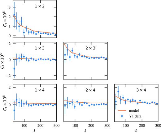
Cross-power spectra among different redshift bins. The number of the redshift bins considered for the cross-power spectra are shown on the top right of each panel. Error bars are computed from the variance of the clustering signal over the 1800 mocks.
The cross-power spectra measurements were not used on the Y1 BAO analysis, and no robustness test was performed on these measurements. We present these results here to show that there is a clustering signal on large scales only for contiguous redshift bins. The amplitude of such a signal is determined by the photo-z distributions overlap between bins (Fig. 1). The clustering signal on small scales appears consistent with zero, showing no indication of further systematic effects affecting shot-noise. The overall agreement between modelling and measurements represents a consistency check for the photo-z distributions of the selected bins.
These correlations could be used in future analysis to constrain, for example, uncertainties in the mean of photo-z distributions.
