Stochastic modelling of star-formation histories I: the scatter of the star-forming main sequence

Caplar, Neven; Tacchella, Sandro

doi:10.1093/mnras/stz1449

ABSTRACT

We present a framework for modelling the star-formation histories of galaxies as a stochastic process. We define this stochastic process through a power spectrum density with a functional form of a broken power law. Star-formation histories are correlated on short time-scales, the strength of this correlation described by a power-law slope, α, and they decorrelate to resemble white noise over a time-scale that is proportional to the time-scale of the break in the power spectrum density, τ_break. We use this framework to explore the properties of the stochastic process that, we assume, gives rise to the log-normal scatter about the relationship between star-formation rate and stellar mass, the so-called galaxy star-forming main sequence. Specifically, we show how the measurements of the normalization and width (σ_MS) of the main sequence, measured in several passbands that probe different time-scales, give a constraint on the parameters of the underlying power spectrum density. We first derive these results analytically for a simplified case where we model observations by averaging over the recent star-formation history. We then run numerical simulations to find results for more realistic observational cases. As a proof of concept, we use observational estimates of the main sequence scatter at z ∼ 0 and M_⋆ ≈ 10¹⁰ M_⊙ measured in H α, UV+IR, and the u-band. The result is degenerate in the τ_break-α space, but if we assume α = 2, we measure |$\tau _{\rm break}=170^{+169}_{-85}~\mathrm{Myr}$|⁠. This implies that star-formation histories of galaxies lose ‘memory’ of their previous activity on a time-scale of ∼200 Myr.

galaxies: evolution, galaxies: star formation, galaxies: statistics

1 INTRODUCTION

Recent observational studies have produced a wealth of data on galaxy populations at different epochs. This has enabled us to study galaxies in a statistical manner and explore scaling relations between a wide range of galaxy properties, such as luminosity, colour, stellar mass, size, velocity dispersion, and central stellar mass density, with cosmic time (e.g. Faber & Jackson 1976; Kormendy 1977; Djorgovski & Davis 1987; Baldry et al. 2004; van der Wel et al. 2014; Barro et al. 2017; Mosleh et al. 2017). However, how and why individual galaxies change their physical properties and evolve to create such scaling relations is still unclear, since we observe each individual galaxy only once during its cosmic lifetime.

A possible way forward is the use of analytical and numerical models. A large body of theoretical work, including cosmological simulations, has been developed aiming to explain the evolving galaxy properties and constrain physical mechanisms that give rise to the observations (e.g. Ceverino et al. 2014; Hopkins et al. 2014; Porter et al. 2014; Vogelsberger et al. 2014; Henriques et al. 2015; Schaye et al. 2015; Pillepich et al. 2018). Currently, such models still have relatively limited predictive power because of the inadequate spatial/mass/temporal resolution, producing small galaxy samples and/or the uncertainties associated with the ‘sub-grid’ physics (e.g. Somerville & Davé 2015).

Another way forward is based on observations: precise evaluation of the number densities of different types of galaxies, coupled with continuity equations, can be used to construct high-fidelity phenomenological models that explain a large number of observed features in the Universe (Peng et al. 2010; Leitner 2012; Carollo et al. 2013; Damjanov et al. 2014; Kelson 2014; Caplar, Lilly & Trakhtenbrot 2015; Kelson, Benson & Abramson 2016; Caplar, Lilly & Trakhtenbrot 2018). Additionally, galaxy stellar ages can be used to understand how galaxies relate to their precursors at earlier epochs to constrain, for example, the mechanism responsible for the change in morphology (Fagioli et al. 2016; Tacchella et al. 2017; Williams et al. 2017; Zahid & Geller 2017; Damjanov et al. 2019).

More general than simple ‘ages’ are star-formation histories (SFHs), which are one of the critical ingredients needed to understand the evolution of galaxies. Having the full information on how galaxies change their star-formation rate (SFR) as a function of cosmic time would allow us to project the galaxy back in time and understand on which time-scales the galaxy grew its mass as a consequence of star formation. Furthermore, SFHs encode information about the variability on short and long time-scales that arise from different physical mechanisms. On long time-scales (>10⁸ yr), physical processes such as gas accretion, mergers, or global gravitational instabilities are expected to play a crucial role, while on shorter time-scales (comparable to and shorter than the galaxy dynamical time) the dynamics of fountains, feedback, and individual giant molecular clouds and star clusters becomes dominant (e.g. Hopkins et al. 2014).

SFHs are related to the scaling relation between the SFRs and stellar masses (M_⋆) of galaxies: observational studies have produced a consensus that since at least redshift 3, the majority of star-forming galaxies have an SFR that is strongly correlated with their mass (⁠|$\mathrm{SFR}\propto M_{\star }^{\beta }$|⁠, with β ∼ 1), creating the so-called star-forming main sequence (MS). It has been established that the MS normalization increases with the lookback time as (1 + z)^∼2.2 (Brinchmann et al. 2004; Daddi et al. 2007; Elbaz et al. 2007; Noeske et al. 2007; Whitaker et al. 2012; Speagle et al. 2014; Schreiber et al. 2015; Boogaard et al. 2018). This increase of the overall normalization of the MS with lookback time can be understood by the higher dark matter accretion rate onto haloes, which leads to higher gas fractions in high-redshift galaxies (Lilly et al. 2013; Tacchella, Trenti & Carollo 2013; Tacconi et al. 2013; Genzel et al. 2015; Rodríguez-Puebla et al. 2016; Tacchella et al. 2018).

The most noticeable feature is that the MS relation at any given redshift shows a rather small scatter of σ_MS ∼ 0.2–0.4 dex, depending on the exact definition of star-forming galaxies and the method used to infer SFRs and stellar masses. This rather small scatter has been used to argue that the SFRs of galaxies on the MS are sustained for extended periods of time in a quasi-steady state of gas inflow, gas outflow, and gas consumption (Bouché et al. 2010; Daddi et al. 2010; Genzel et al. 2010; Davé, Finlator & Oppenheimer 2012; Lilly et al. 2013; Dekel & Mandelker 2014; Rodríguez-Puebla et al. 2016; Tacchella et al. 2016). Clearly, the MS scatter is directly related to the variability in the SFH and hence encodes physical mechanisms acting on different time-scales. In general terms, Abramson et al. (2015, see also Muñoz & Peeples 2015) highlight that if the MS scatter arises due to short-term fluctuations, star-forming galaxies with similar mass mostly grew-up together, while if the MS scatter arises due to long-term fluctuations (Peng et al. 2010; Behroozi, Wechsler & Conroy 2013), then star-forming galaxies with similar mass did not grow-up together and key physics lies in the process that diversifies star formation histories (Gladders et al. 2013; Kelson 2014).

Based on cosmological zoom-in simulations (VELA simulations; Ceverino et al. 2014; Zolotov et al. 2015), Tacchella et al. (2016) suggested that star-forming galaxies with M_⋆ ≈ 10⁹–10¹¹M_⊙ oscillate about the MS ridgeline on time-scales of ≤2 Gyr at z ∼ 1–4. The propagation of galaxies upwards towards the upper envelope of the MS is due to gas compaction, triggered by e.g. mergers, counter-rotating streams, and/or violent disc instabilities. The downturn at the upper envelope is due to central gas depletion by peak star formation and outflows while inflow from the shrunken gas disc is suppressed. Rodríguez-Puebla et al. (2016) argue, based on advanced abundance matching, that the MS scatter could be set by the halo mass accretion rate, which itself has a scatter of ∼0.3 dex, matching the observed dispersion of the MS. Matthee & Schaye (2019) show, based on the EAGLE simulations, that the scatter of the MS at z ∼ 0 originates from a combination of short time-scales (⁠|${\lesssim}1~\mathrm{Gyr}$|⁠) that are presumably associated with self-regulation from cooling, star formation and outflows, and long time-scale (∼10 Gyr) variations related to differences in halo formation times. Torrey et al. (2018) show, based on the IllustrisTNG simulations, that galaxy offsets from the MS and mass–metallicity relation oscillate over similar time-scales (roughly the dynamical time of the dark matter halo) and are often anticorrelated. They speculate that the SFR and metallicity evolution tracks may become decoupled in galaxy formation models dominated by feedback-driven globally bursty SFHs, which could weaken the FMR residual correlation strength.

It is well-known that measurements of SFR in different observed bands carry different information, with shorter wavelengths carrying more information about recent star-formation, and longer wavelengths being more sensitive to star-formation on longer time-scales (e.g. Boquien, Buat & Perret 2014). However, measuring SFHs from the observed spectral energy distribution (SED) of galaxies is still very challenging (Conroy 2013). State-of-the-art SED fitting codes are nowadays able to fit non-parametric SFHs to the galaxy SEDs and provide constraints of the SFHs on time-scales of 100 Myr to a few Gyrs, i.e. on rather long time-scales (Thomas et al. 2005; Graves & Schiavon 2008; Davies et al. 2015; Pacifici et al. 2016; Iyer & Gawiser 2017; Leja et al. 2019a; Carnall et al. 2019). Short time-scales can in principle be inferred from comparing nebular lines to the ultraviolet (UV) continuum. For instance, Weisz et al. (2012), Guo et al. (2016), Emami et al. (2018), and Broussard et al. (2019) inferred a systematic decline and increased scatter in nebular line to FUV ratios towards low-mass systems. They interpreted their data with simple SFH models that included bursts lasting tens of Myr, and with periods of ∼250 Myr, finding that these low mass galaxies are rather ‘bursty’. However, large uncertainties remain, including variations of the initial mass function (IMF), differential dust attenuation distribution in front of young and old stars, and metallicity effects (e.g. Shivaei et al. 2018). A different way forward, specifically for constraining the time-scales involved in the star-formation processes, such as lifetime of the molecular clouds, includes studying the scaling relation between the gas mass and SFR on spatially resolved scales (Kruijssen & Longmore 2014; Kruijssen et al. 2018).

All this research implies that galaxies exhibit wide range of SFHs, exhibiting bursts, drops, and periods non-changing star-formation. In this work, we propose to model the time-dependence of star formation and the movement of star-forming galaxies around the MS ridgeline as a purely stochastic process. We aim to describe the stochastic behaviour in very general terms and therefore define its properties in the frequency domain through a power spectrum density (PSD) that is modelled as a broken power law. The high-frequency slope of the PSD determines how quickly the SFR changes on short time-scales and is going to be connected with physical drivers of star-formation. The broken power-law form allows for a break in the correlation, i.e. sets up a time-scale on which the SFR in a single galaxy loses ‘memory’ of previous star-formation.

We note that this time-scale can, in principle, be longer than the time-scale of the Universe. In that case, the PSD is effectively a pure power law for all practical purposes and the star formation in a given galaxy has a ‘long-term dependence’, i.e. it is correlated over the cosmic time-scales. This process, with a single power-law slope, is used by Kelson (2014) to model stellar mass growth in the Universe. He described the SFHs using a so-called ‘Hurst parameter’, which is very closely related to the slope of the PSD used in this work. We discuss the connection between describing the stochastic process via the PSD with a broken power law (and its high-frequency slope) and the description using ‘Hurst parameter’ more extensively in Appendix A.

In this paper we focus on the Myr to a Gyr time-scale and exclude the longer time-scales in the analysis, which we believe set the overall evolution of the MS. We are therefore considering only the regime in which ‘short-term fluctuations’ are dominant. Characterization of the PSD on these ‘short’ scales is critical for a couple of reasons. First, it provides a test for simulations, which aim to match various distributions (e.g. galaxy mass function) over a span of redshifts, but do not necessarily aim to match stochasticity of star-formation with cosmic time. Secondly, the recovered parameters of the underlying stochastic process are connected to the physical drivers of star-formation and can provide valuable insight into the properties of star-formation (e.g. Faucher-Giguère 2018). In particular, the time-scale of the break in the PSD should be connected with the time-scale on which star formation due to internal galaxy properties becomes less important compared to external feeding of the galaxy. For an example in a related field, stochastic modelling of the short-term variability (∼1 yr) of active galactic nuclei (AGN) is one the main methods to explore physical processes powering AGN (Kelly, Bechtold & Siemiginowska 2009; MacLeod et al. 2010; Dexter & Agol 2011; MacLeod et al. 2012; Simm et al. 2016; Caplar, Lilly & Trakhtenbrot 2017), and is providing serious challenges to standard viscous accretion disc models commonly used to model AGN accretion (see review by Lawrence 2018). Finally, understanding the variability of the SFR on short time-scale is crucial for proper SED fitting, as the characteristic time-scale on which SFR varies is directly related to the size of parameter confidence intervals (Leja et al. 2019b).

In this work we lay the basic groundwork of our approach and conduct a simple analysis of the observations in order to constrain the PSD. We take purely observational approach to determining the parameters of the underlying stochastic process and leave the discussion of the possible physical interpretation for the future work.

We focus our investigation on rather massive star-forming galaxies with M_⋆ ≈ 10¹⁰–10^10.5 M_⊙. We work in this rather narrow mass range because measurement errors are the small, fraction of galaxies that are quenching is negligible, and result are being less affected by possible variations of dust attenuation with galaxies mass (as elaborated in Section 5). In a companion paper (Iyer et al., in preparation), we analyse and measure the PSDs for a wide range of numerical (cosmological and zoom-in simulations) and semi-analytical models. We find that PSDs are well described by a broken power law, where the short time-scales (high frequencies) follow ∝ f^α and above a certain decorrelation time-scale, τ_break, the PSD is constant. Nearly all of the different theoretical models produce α ≈ −2, while having different values for τ_break, ranging from τ_break ∼ 100 Myr in the FIRE simulations to τ_break ∼ 1000 Myr in IllustrisTNG. We show that the PSD is set by physical ingredients in the models and, hence, the PSD contains a wealth of information that has not yet been exploited. In a separate, upcoming paper we will address many issues that complicate the precise determination of the PSD in observations, including possible variations in the IMF and dust attenuation. There, we also wish to use observational constraints to analyse properties of galaxies at higher redshifts, where the proper consideration of these complications is critically important.

This paper is structured as follows. In Section 2 we introduce our model and give a short overview of the properties of stochastic processes. In Section 3 we show how we can infer parameters describing movement of galaxies about the MS. We show both analytical and numerical results in the simplified case in which response of each star-formation indicator is given by a step function. In Section 4 we show predictions for the observational results given the more realistic response functions. In Section 5 we use results developed in previous sections and determine, as a proof of concept, parameters describing stochastic processes by using observations of the measured scatter of the MS in the local universe. We conclude in Section 6. In the appendix we expand on several more technical aspects of the paper.

Throughout the paper we use the terms ‘scatter of MS’, ‘standard deviation of MS’, and ‘width of MS’ interchangeably, and denote it by σ_MS. We use the term ‘intrinsic’ MS, or ‘momentary’ MS to denote width of the MS that would be detected if we could measure the star-formation over the previous 1 Myr. We expand on our choice for 1 Myr in Section 2.3. We make our codes available at github.com/stacchella/ and github.com/nevencaplar/.

2 DESCRIPTION OF STAR-FORMATION HISTORIES WITH STOCHASTIC PROCESSES

In this section, we introduce our approach to modelling SFHs with stochastic processes. In particular, we start by highlighting and justifying the assumptions we make in our model. We then explain what a stochastic process is and how it can be described mathematically. Finally, we show how we generate SFHs with a stochastic process and discuss their properties such as burstiness.

2.1 Assumptions

We propose to model time dependence of the SFR relative to the MS ridgeline of star-forming galaxies as a purely stochastic process. We denote the SFR relative to the MS ridgeline for a galaxy with stellar mass M_⋆ by Δ_MS = log (SFR/SFR_MS(M_⋆)), where SFR_MS(M_⋆) is the SFR of the MS at mass of M_⋆. Throughout this work, we assume that:

there exists an MS, i.e. there is a power-law relation between SFR and stellar mass for star-forming galaxies that are separate from the quiescent galaxy population;
the distribution of SFRs of galaxies about the MS ridgeline is well described by a log-normal function;
time-variability of Δ_MS of all star-forming galaxies of a given mass can be described with the same stochastic process given by a broken power-law PSD.

The first two assumptions are well justified from observations. Specifically, the existence of the MS have been put forward by several different observing groups (e.g. Daddi et al. 2007; Elbaz et al. 2007; Noeske et al. 2007; Peng, Maiolino & Cochrane 2015). Furthermore, several groups claim that the scatter can be well described by a log-normal (Guo, Zheng & Fu 2013; Chang et al. 2015; Schreiber et al. 2015; Davies et al. 2019). Feldmann (2017) shows that the whole galaxy population, i.e. star-forming and quiescent galaxies, can be well fitted by a zero-inflated negative binomial distribution, which is only a small modification from the log-normal distribution describing star-forming galaxies, but has the advantage that no division between star-forming and quiescent galaxies is needed. There is still a debate in the literature about the exact shape of the MS, including its slope and turnover at high mass at low redshifts, and also about the existence of an MS at high redshifts (z > 3; Speagle et al. 2014; Whitaker et al. 2014; Iyer et al. 2018). As such, additional considerations need to be applied when working at those high redshifts. Similarly, at masses where the number of quenching galaxies starts to be comparable to the number of star-forming galaxies, one needs to be careful to not confound the contribution of the tail of the quenching galaxies to the ‘intrinsic’ log-normal distribution of the star-forming galaxies. We focus, in this paper, on moderately massive (≈10¹⁰ M_⊙) galaxies at z ∼ 0 and model the SFRs relative to the MS. We show in Section 5.1 that the fraction of galaxies that we expect to be quenching during the inferred time-scale of variability about MS is around 2 |${{\ \rm per\ cent}}$| for the data set from Davies et al. (2019) analysed in this work. The distribution of the galaxies around the MS in the data set is highly consistent with the log-normal distribution. We note here that the fact that the galaxies are log-normally distributed does not necessarily imply that distribution of each and every galaxy around the MS can be described with log-normal distribution – we will show that there are parts of parameters space where individual galaxies are constantly above or below the MS, but the population can be described with a log-normal description.

Number of works (Abramson et al. 2015; Eales et al. 2017; Abramson et al. 2018) proposed modelling global star-forming density on cosmological time-scales as a superposition of many galaxies with loosely constrained lognormal SFHs. Such models reproduce the MS, and the wide distribution of galaxies around the ridgeline of the MS, without any stochastic contribution to the observed diversity of the observed SFRs. As such, our approach which is modelling stochastic movement, would not be directly applicable. We note however, that our modelling offers great flexibility in modelling wide variety of SFH and that parts of the parameter space that we explore (where τ_break and α are both large, giving non-bursty SFH; see below) reproduces similar SFHs as expected from these models. In Appendix B we discuss the hybrid model, i.e. the effect of the global evolution of the star-formation mixed with the stochastic evolution, but we leave full comparison of the two approaches (deterministic log-normal histories of individual galaxies and stochastic movement around MS) for the future work.

The third assumption listed above, that all massive star-forming galaxies are described with the same stochastic processes, is the simplest reasonable assumption and it enables us to maintain analytical tractability of the model. In this work we do not explore further variables that could influence the PSD, such as environment. It is also possible that lower mass galaxies (including dwarfs) follow a stochastic process with different properties; this will be investigated in the future. Finally, as also mentioned in the introduction, we assume that the stochastic behaviour can be described through a broken power-law PSD, i.e. we assume that the 3-point correlation function (and any higher order terms) is zero. This is again a reasonable assumption given the current observational constraints, as further discussed in Section 5.

2.2 General description of stochastic processes

In this section, we will discuss several different stochastic processes and develop an intuition for parameters that we will use in the rest of paper. We characterize different stochastic processes by their PSD, a quantity denoting the amount of power that a process has as a function of frequency, per unit frequency. The PSD gives a quantitative estimate of the importance of each mode, i.e. the importance of each frequency interval for a given stochastic process. We will also extensively use the Fourier pair of the PSD, the autocorrelation function (ACF). The ACF provides the same information as the PSD, but in the time domain instead of the frequency domain. The definition of ACF, for a process that leads to a time-series Δ(t) is

\begin{eqnarray*} \mathrm{ ACF}(\delta t)= \frac{\lim _{T \rightarrow \infty } \frac{1}{T} \int _{(T)} \Delta (t) \Delta (t+\delta t)\, \mathrm{ d}t}{\sigma ^{2}_{ \Delta }}, \end{eqnarray*}

(1)

where |$\sigma ^{2}_{ \Delta }$| is the long-term variance of the process. We can see that highly correlated time-series, where Δ(t) ∼ Δ(t + Δt), give ACF ∼ 1, while uncorrelated time-series will lead to ACF ∼ 0.

The simplest stochastic process is white noise. This process has equal power at all frequencies. In this work, we denote frequency with f. The statement about equal power on all frequencies can be mathematically written as PSD(f) ∝ f^α, with α = 0. This process is perfectly uncorrelated, i.e. for a white noise process it holds that ACF(t) = 0, for all times when t > 0.

Other processes can be defined by modifying the slope α of the PSD. By decreasing the slope α, the nature of process changes and values separated by a given Δt become more similar. Some well known examples are given by α = −1 (pink noise) and by α = −2 (red noise); the latter corresponding to a random walk or Brownian motion.

All natural process have some characteristic time τ, after which a process becomes uncorrelated, i.e. loses its ‘memory’ of the previous values and behaves like a white noise process. We can express that statement in terms of the ACF by saying that the ACF at times longer than the decorrelation time, τ_decor has to be very small, ACF(t > τ_decor) ≪ 1, or, in the closely related terms of the PSD, by requiring that the slope at small frequencies below ‘break’ frequency, f_break, has to be close to zero, α(f < f_break) ≈ 0. In that case, the PSD has a broken power-law shape, with two distinct slopes at large and small frequencies.

To illustrate this point further, let us consider the simplest and most instructive case where the PSD is described by a broken power law, which corresponds to a damped random walk. The damped random walk is defined by the solution to the stochastic differential equation (Kelly et al. 2014):

\begin{eqnarray*} \frac{\mathrm{ d} \Delta (t)}{\mathrm{ d}t}+\frac{1}{\tau _{\rm decor}} \Delta (t)=\epsilon (t), \end{eqnarray*}

(2)

where ϵ(t) is a continuous white-noise process with zero mean and variance |$\sigma _{\rm int}^{2}$|⁠. In this form, one can recognize |$\sigma _{\rm int}^{2}$| as an intrinsic amount of ‘randomness’ entering the system, while τ_decor describes the time-scale by which the process gravitates towards a stable-state solution. This process is also known as the Orstein-Uhlenbeck process in physics, or the Vasicek model in financial literature.

The damped random walk process leads to the following PSD:

\begin{eqnarray*} \mathrm{ PSD} (f) &=& \frac{\sigma ^{2}_{\rm int}}{ 1/\tau ^{2}_{\rm decor}+(2 \pi f)^{2}}\nonumber\\ &=& \frac{\sigma ^{2}}{1+(\tau _{\rm break} f)^{2}}, \end{eqnarray*}

(3)

where σ = σ_intτ_decor is the ‘long-term’ variability and τ_break = 2πτ_decor. The connection of the description of the process in frequency and time domain can be achieved via the Wiener–Khinchin theorem (Emmanoulopoulos, McHardy & Uttley 2010). Application of this procedure for this particular choice of PSD leads to

\begin{eqnarray*} \mathrm{ ACF}(t) = \exp (-t/\tau _{\rm decor}). \end{eqnarray*}

(4)

We see that this process has all the properties that we mentioned above. At short time-scales (high frequencies), it is very well correlated (ACF ∼ 1) and described with a PSD with a slope that equals to 2. Then, the process becomes rapidly decorrelated at a time-scale τ_decor, and at long time-scales (low frequencies), the ACF drops quickly (ACF ∼ 0) and the PSD is well described with a flat slope. Observationally, high values of ACF imply similar measurements, while decorrelation implies little to no similarity between two measurements. As such, while at short time-scales star-formation measurements will be very similar, at time-scales larger than τ_decor the observations of the same galaxy will have star-formation measurements which are largely independent of each other.

In this work, we consider a larger group of processes, described with

\begin{eqnarray*} \mathrm{ PSD} (f) = \frac{\sigma ^{2}}{1+(\tau _{\rm break} f)^{\alpha }}. \end{eqnarray*}

(5)

This choice offers additional flexibility to encompass a wide range of physical processes that are not necessarily described by random walks, providing a more general description of the possible underlying stochastic process. We show examples of generated SFHs relative to the MS, Δ_MS, in Fig. 1. The generation of these SFHs is described in the next section. Figure shows simulated SFHs as a function of high-frequency slopes of the PSD (α in equation 5)¹ and break time-scales (τ_break in equation 5). The figure highlights large qualitative differences between SFHs generated with different parameters. When the slope of the PSD is shallow and/or τ_break is small, the SFH rapidly oscillates around the mean and is very quickly decorrelated. On the other hand, steeper slopes and longer τ_break lead to slower oscillations and more correlated behaviour, as described above. In Section 2.4, we will return to this point in order to quantify the ‘burstiness’ of these processes.

Figure 1.

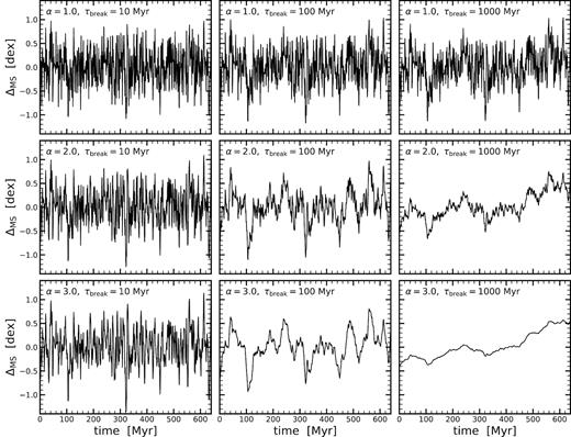
Example star-formation histories (SFHs) drawn from different power spectral densities (PSDs). All of these have been created with the same random seed so they are directly comparable. Each panel shows the SFH relative to the MS ridgeline (Δ_MS), measured with cadence (time-separation) of 1 Myr. From top to bottom, we show the SFHs generated with different PSDs with increasing power-law slope (α = 1 → 3) and increasing break time-scale (τ_break = 10 → 1000 Myr). Overall, the burstiness increases towards smaller α and shorter τ_break.

Open in new tab Download slide

All of the examples shown in Fig. 1 have been created with σ = 0.4 dex. We use this value motivated by the measurement of the MS width in Davies et al. (2019) in H α, and we show in Section 4 that the measurement in H α is largely representative of the intrinsic width of MS,σ_MS. A number of results that we will derive depend somewhat on the intrinsic width of MS. In the rest of the paper, we work with σ_MS = 0.4 dex, but note at each point where our results depend on the exact choice of this value.

Finally, we note that we are implicitly assuming that the stochastic process that we are using is stationary. A stationary process has the property that its mean, variance, and ACF are not time dependent. That the variance, i.e. the width of MS is not time dependent over last several Gyr is consistent with observational data and simulations (Noeske et al. 2007; Rodighiero et al. 2010; Katsianis et al. 2019). In other words, we assume that the properties of stochastic process do not change with time and that is valid to use the same parameters to describe observations of galaxies over the whole time range probed. It is important to note that this does not mean that we assume that the MS is not allowed to change with time. The main stochastic process modelled in this work is movement of galaxies about the MS ridgeline (Δ_MS). The MS itself evolves over cosmological time-scales, but because we consider galaxies at z = 0, this evolution is negligible. We further discuss this effect in Section 5, when comparing the results from our modelling with the observational data.

2.3 Generating star-formation histories

Here we describe how we generate numerically a sample of SFHs that we use in the rest of the paper when we analyse properties of stochastic processes and observational consequences. For each choice of break time-scale τ_break and high-frequency slope α we simulate 1000 SFHs using the algorithm by Timmer & Koenig (1995) and implemented in Python by Connolly (2015). This standard method works by inverse Fourier transforming the supplied PSD to give an ensemble of stochastic time-series. It is a robust method that correctly reproduces intrinsic scatter in the power at given frequency by randomizing both the phase and the amplitude of the Fourier components. Further discussion of the strengths and weakness of the method is available in Emmanoulopoulos, McHardy & Papadakis (2013). For each galaxy, we only consider the SFR as an integrated quantity over the whole galaxy, i.e. we measure only total SFRs over the whole galaxy without deeper considerations of possible difference in different galactic (sub-)components.

When simulating SFHs we need to assume some minimal time-scale at which to separate our measurements of SFR (time bins). In this work we set this time-scale to 1 Myr. This choice is motivated by the free-fall time and the lifetime of giant molecular clouds which are at least of that order (Murray, Quataert & Thompson 2010; Hollyhead et al. 2015; Freeman et al. 2017; Grudić et al. 2018). Operationally this means that we are assuming that below the scale of 1 Myr, the SFR is perfectly correlated, i.e. remains constant. This is a reasonable assumption since we are considering only total SFRs integrated over the whole galaxy, which itself is made up of several star-forming events (giant molecular clouds). In terms of PSD that means that the domain of the PSD is defined up to scales of f < 1/Myr. In terms of ACF this leads to a discontinuity in our assumed ACF at 1 Myr, where we set ACF to be equal to unity. The effect of this assumption is less and less pronounced when the stochastic process has larger α and τ_break, since in this case the process is already highly correlated on 1 Myr scales, and our assumption is satisfied by construction. In Section 5, when we compare with observational data at low redshifts, the deduced parameters are outside the range that is critically sensitive to this assumption, but this might not be the case for studies at higher redshifts where deeper investigation of this assumption should be conducted.

For each SFH we simulate 4282 points, corresponding to 4.282 Gyr, i.e. to a galaxy evolving from z = 0.4 to z = 0. We note that choice of the length is somewhat arbitrary and carries no great physical significance. Our results are not dependent on the actual duration of the simulated histories, provided they are significantly longer than the τ_break of the considered process. In Fig. 2 we illustrate the results of this procedure. For each τ_break and α, we show a selection of three SFHs relative to the MS (left-hand panel), together with their PSDs and ACFs (middle and right-hand panels). We also show median relations in black, which have been deduced from all 1000 simulated galaxies. We also explicitly show the effect of a cut at 1 Myr, seen as the grey region in the plots of the PSD, and seen in the fact that ACFs extended ‘only’ to log (time/Myr) = 0.

Figure 2.

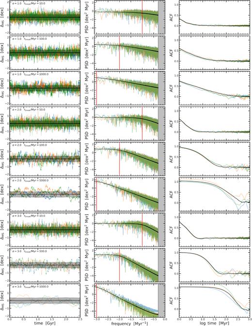
Example SFHs relative to the MS, associated PSDs and ACFs. From top to bottom, we show SFHs with increasing slope (α = 1 → 3) and increasing break time-scale (τ_break = 10 → 1000 Myr). The left-hand panels show the SFHs relative to the MS as a function of time. Three, randomly drawn, examples are shown with blue, orange, and green lines. The solid black line and the grey shaded region show the mean and scatter of the MS of our 1000 model galaxies. Given the large number of galaxies in the simulations, the mean relation and the scatter change very little with time. The middle panels shows the associated PSDs; the black line shows the median PSD of our 1000 model galaxies. The vertical red line indicates τ_break, while grey region indicates our resolution limit at which we truncate the PSDs. The right-hand panels show the associated ACFs and the black line shows the median ACF for our 1000 model galaxies.

Open in new tab Download slide

2.4 Quantifying the burstiness of star-formation histories

Here we want to connect the parameters that we have introduced (α and τ_break) with a more intuitive quantity which describes the tendency of the SFH to have ‘bursts’, i.e. periods of star formation which are much higher (or lower) than the mean of the population. From Figs 1 and 2 it is apparent that the power-law slope α and the break time-scale τ_break are connected with the variability, or ‘burstiness’, of the SFH. Following Goh & Barabási (2008, see also Applebaum et al. 2018), we define the burstiness parameter, for a single galaxy, as

\begin{eqnarray*} B = \frac{\sigma /\mu -1}{\sigma /\mu +1}, \end{eqnarray*}

(6)

where σ is the standard deviation of Δ_MS, and μ is the mean of Δ_MS of an individual SFH, measured over a certain time interval. It is important to note that the exact value of B depends on the interval over which it is measured. We choose this time interval to be 30 Myr in order to have the dynamic range to describe the large diversity of variability seen in Fig. 1. This choice of time interval is also consistent with the one used by Applebaum et al. (2018). In general, B has a value in the bounded range (−1, 1), and its magnitude correlates with the signal’s burstiness. The average deviation from the MS for one galaxy, μ, will approach zero as the SFH becomes more bursty. Therefore, B = 1 is a maximally bursty signal, B = 0 is neutral, and B = −1 corresponds to a completely regular (periodic or constant) signal.

To show trends as a function of α and τ_break, we compute the mean of B over our sample of 1000 numerically generated model galaxies for each point of the α-τ_break parameter space. Fig. 3 shows how the burstiness B varies as a function of the PSD parameters α and τ_break. Large values of α and τ_break correspond to slowly varying, nearly constant SFHs (see Fig. 1), corresponding to B = −1, i.e. highly non-bursty. Most individual galaxies rarely venture to the edges of the MS and therefore experience no episodes of very high (or very low) SFR in comparison to the average over 30 Myr. On the other hand, PSDs with small α and short τ_break produce SFHs with B = 1 (highly bursty). These SFH rapidly change their SFR and have very varied SFHs over the considered time range of 30 Myr. Furthermore, Fig. 3 highlights the degeneracy between α and τ_break: contours of constant B extend along well-defined curves in the α-τ_break plane. This is something that we will encounter again in Sections 3 and 4, where we investigate how the scatter of the MS as seen from different indicators depends on the PSD parameters α and τ_break.

Figure 3.

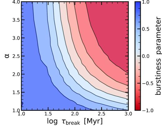
The burstiness parameter B. We plot the burstiness parameter (equation 6) estimated for the different PSDs with power-law slope α and break time-scale τ_break. PSDs with low values of α and τ_break yield highly bursty (B = 1) SFHs, while PSDs with high values of α and τ_break give constant and hence regular (B = −1) SFHs. There is a clear degeneracy between α and τ_break.

Open in new tab Download slide

3 FINDING PARAMETERS OF STOCHASTIC STAR-FORMATION HISTORY IN A TOY MODEL

In the previous section we have shown how different choices for parameters describing the PSD (namely the slope α and the break time-scale τ_break) lead to different SFHs of star-forming galaxies. Estimating these stochastic parameters from observations is difficult, since it is still a big challenge to infer the SFH from a galaxy’s SED (see Introduction). By measuring the SFR using different indicators we are able to estimate how the SFR varied in the galaxy’s recent past (e.g. Kennicutt 1998). Specifically, measurements of the SFR with indicators that are based on nebular lines will probe very recent star-formation (∼10⁶ yr), while measurement in the UV and optical bands will be sensitive to much longer time-scales (∼10⁷ and ∼10⁸yr, respectively; see also Section 4). As we will show below, by studying a large sample of galaxies for which the SFRs have been estimated with different indicators, the parameters of the underlying stochastic process can be deduced.

To develop understanding, we present the simplest possible case in which measurements with different indicators correspond exactly to averaging the recent SFR over a given time-scale. We will develop analytical expressions for the offset as well as scatter of the MS as a function of the averaging time-scale. This approach will help us to see connections and correlations between different parameters more clearly. This type of averaging procedure is equivalent to the analysis conducted by Hopkins et al. (2014, see fig. 12 there), who showed significant changes in the inferred scatter as a function of the averaging time. Afterwards, in Section 4, we discuss realistic response functions for different SFR indicators and redo much of the calculations with more complex and more realistic models. In contrast with mainly analytical approach in this section, when dealing with more realistic cases we will derive results with greater emphasis on numerical calculations.

3.1 Impact of averaging of the star-formation histories on the shape of the measured MS

In this section we show how the measured normalization and width of the MS change as a function of the time-scale over which the SFH is averaged. These changes depend on the properties of the stochastic process (i.e. PSD) and, hence, can also be used to infer these properties. We first show analytically derived relations between the measured offset from the MS and then the expression for the width of the MS. We then confirm these results by our numerically generated model galaxies (Section 2.3) and show how parameters of stochastic process can be deduced from measurements.

3.1.1 Mean measured offset from the main sequence

We first consider mean offsets from the MS, as a function of the parameters of the stochastic process, when measured by indicators probing different time-scales. We denote the SFR that has been measured with a given indicator by |$\mathrm{SFR_{\rm ind}}$|⁠. As already mentioned, we assume now the simplest possible case in which the response of each indicator is given by a step function each with different lengths, i.e. different response times. In that case, the response step function can be divided into N_j equal time-steps. The measurement of the SFR with a given indicator at time t_i is then equal to the averaged ‘true’ SFR of the previous N_j steps, where t_j are labels for these equidistant time-steps:

\begin{eqnarray*} \mathrm{SFR}_{\rm ind}(t_{i})=\frac{1}{N_{j}} \sum ^{N_{j}}_{t_{j}=1}\mathrm{SFR}(t_{i}-t_{j}). \end{eqnarray*}

(7)

Let us now define the logarithmic distance of the SFR from the ridgeline of the intrinsic MS²

\begin{eqnarray*} \Delta (t_{i}) =\log \mathrm{SFR}(t_{i}) - \log \mathrm{SFR}_{\rm MS}(M_{\star },t_{i}), \end{eqnarray*}

(8)

and its equivalent quantity, logarithmic distance of measured SFR from the ridgeline of intrinsic MS

\begin{eqnarray*} \Delta _{\rm ind}(t_{i}) =\log \mathrm{SFR}_{\rm ind}(t_{i}) - \log \mathrm{SFR}_{\rm MS}(M_{\star },t_{i}). \end{eqnarray*}

(9)

In this work we are also assuming that the time and mass dependence of log SFR_MS(M_⋆, t) can be neglected, i.e. log SFR_MS(M_⋆, t) ≡ C, where C is a constant in units of M_⊙ yr⁻¹. This is done to simplify the calculation and is indeed true at low redshifts (see further discussion in Section 5.2.2).

By combining equations (7), (8), and (9) we find that

\begin{eqnarray*} \Delta _{\mathrm{ind}}(t_{i}) &=& \log \frac{1}{N_{j}} \sum ^{N_{j}}_{t_{j}=1} \mathrm{SFR} (t_{i}-t_{j}) - \log \mathrm{SFR}_{\rm MS} \nonumber\\ &=& \log \frac{1}{N_{j}} \sum ^{N_{j}}_{t_{j}=1} 10^{\Delta (t_{i}-t_{j})+\log \mathrm{SFR}_{\rm MS}}- \log \mathrm{SFR}_{\rm MS} \nonumber\\ &=&\log \frac{1}{N_{j}} \sum ^{N_{j}}_{t_{j}=1} 10^{\Delta (t_{i}-t_{j})}. \end{eqnarray*}

(10)

The above expression is true for a single galaxy, but in observations we are looking for a statistical quantity 〈Δ_ind(t_i)〉, where we use 〈〉 to denote the average value of the measured offset from MS, i.e. to denote that the measurement has been averaged over a sample of observed galaxies.

〈Δ_ind(t_i)〉 can be explicitly derived for the case of damped random walk (equations 2 and 3). When the galaxy is at an MS distance of Δ(t_j) at some time t_j, its expected distribution at later time t_i − t_j is given by (Kelly et al. 2009; MacLeod et al. 2010):

\begin{eqnarray*} && {P [\Delta (t_{i}-t_{j})]}\nonumber\\ && {\quad = \mathcal {N} \left(\Delta (t_{j}) \exp \left(-\frac{t_{i}-t_{j}}{4 \tau _{\rm decor}}\right) , \sigma _{\rm MS} \sqrt{1-\exp \left(-\frac{t_{i}-t_{j}}{2 \tau _{\rm decor}}\right) }\,\right) ,}\nonumber\\ \end{eqnarray*}

(11)

where with P we denote expected distribution and |$\mathcal {N}(\mu ,s)$| denotes a normal distribution with mean μ and standard deviation of s. We are actually interested in the quantity that appears in equation (10), i.e. the expectation value of the quantity |$10^{\Delta (t_{i}-t_{j})}$|⁠. The expectation value, E, for a lognormal distribution is given by

\begin{eqnarray*} E[10^{\mathcal {N}(\mu ,s)}] =10^{\mu + \frac{s^{2} \ln (10)}{2}}. \end{eqnarray*}

(12)

Therefore, the expectation value of the process at time t_i − t_j is given by

\begin{eqnarray*} E[10^{\Delta (t_{i}-t_{j})}]= 10^{\Delta (t_{j}) \exp \left(-\frac{t_{i}-t_{j}}{4 \tau _{\rm decor}}\right) +\sigma ^{2}_{\rm MS} \left(1-\exp \left(-\frac{t_{i}-t_{j}}{2 \tau _{\rm decor}}\right)\right) \frac{\ln (10)}{2} }. \end{eqnarray*}

(13)

Combining together the expressions from equations (10) and (13) we obtain:

\begin{eqnarray*} &&\langle \Delta _{\rm ind} (t_{i})\rangle\nonumber\\ &&\quad= \log\!\! \left(\!\frac{1}{N_{j}} \!+\! \sum^{N_{j}}_{t_{j}=1} 10^{\Delta (t_{j}) \exp \Big(\frac{-(t_{i}-t_{j})}{4 \tau _{\rm decor}}\Big)+ \sigma^{2}_{\rm MS} \Big(1-\exp \Big(\frac{-(t_{i}-t_{j})}{2 \tau _{\rm decor}}\Big)\Big) \frac{\ln (10)}{2}}\!\right)\!\!.\nonumber\\ \end{eqnarray*}

(14)

We see that the measured offset depends on the duration of the response of an indicator (N_j), the properties of underlying stochastic process (only τ_decor in case of the damped random walk) and the intrinsic width of the main sequence (σ_MS). We can also see that larger offsets are realized for larger values of N_j, τ_decor and σ_MS. We will investigate the interplay of these parameters more closely in Section 3.2.

3.1.2 Width of the MS

We now turn to the width of the MS and explore this property as a function of parameters of the stochastic process. The derivation is somewhat involved; see Appendix C for details. There we show that the lowest order expansion, as a function of σ_MS, of the measured variance of a sample of galaxies, |$\sigma ^{2}_{\rm ind,MS}$|⁠, is given by

\begin{eqnarray*} \sigma ^{2}_{\rm ind, MS} (t_{i})=\frac{\sigma ^{2}_{\rm MS}}{N^{2}_{j}} \sum _{t_{j}=1}^{N_{j}}\sum _{t_{j^{^{\prime }}}=1}^{N_{j}} ACF (t_{j}-t_{j^{^{\prime }}}), \end{eqnarray*}

(15)

where σ_MS is the intrinsic width of the MS. This double summation can be simplified by using symmetry properties of the autocorrelation function, to yield the measured σ_{ind, MS} (Priestley 1981; Ivezić, Connolly, Vanderplas, and Gray 2014):

\begin{eqnarray*} \sigma _{\rm ind, MS} (t_{i})=\frac{\sigma _{\rm MS}}{\sqrt{N_{j}}} \left(1 + 2 \sum ^{N_{j}}_{t_{j}=1} \left(1-\frac{t_{j}}{N_{j}} \right)\mathrm{ ACF}(t_{j}) \right)^{1/2} . \end{eqnarray*}

(16)

We note that this equation has the same form as the equation for the uncertainty of the mean for the data set consisting of N_j measurements with a homoscedastic measurement error of σ_MS. This is another intuitive way to think about this quantity that we are measuring. In essence, we are exploiting the ergodic property of our sample. Measuring the width of the distribution created by galaxies that are moving stochastically around the MS with an indicator over N_j times is equivalent to measuring the mean of a sample of galaxies on MS at N_j different times!

We see that in case of ACF(t_j) = 0, the expression in the brackets of equation (16) is unity, and therefore the measured scatter of the MS drops very quickly as |$\sigma _{\rm MS}/\sqrt{N_{j}}$|⁠, which is the familiar expression for the uncertainty of the mean from any analysis that uses independent measurements. On the other hand, in case of highly correlated data (ACF(t_j) ≈ 1), the measured scatter of the MS is essentially unchanged and corresponds to the initial σ_MS.

3.2 Comparison to numerically generated model galaxies

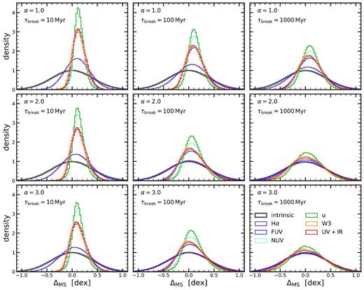
We now consider the consequences of the theory developed above, i.e. we study the interplay between the stochastic process of star-formation and the time-scale of the indicators used to probe the SFR. We show in Fig. 4, as a function of PSD parameters, how the shape of the MS (i.e. distribution of Δ_MS at fixed mass) depends on the different averaging time-scale. The grey line, which is the same in all panels, shows the intrinsic distribution of the 1000 model galaxies about the MS ridgeline (Δ_MS). By construction, this intrinsic distribution is defined in 1 Myr time bins and is a normal distribution with σ_MS = 0.4 dex.

Figure 4.

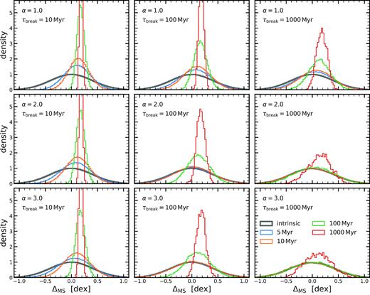
Distribution about the MS ridgeline after averaging the SFHs. Each panel shows the resulting distributions for a given PSD, with increasing α and τ_break from top left to bottom right. The thick black histogram indicates the intrinsic distribution, which has by construction a mean of 0.0 and a scatter of 0.4 dex for all α and τ_break. The blue, orange, green, and red histograms show the distribution of galaxies after their SFHs were averaged over a time-scale of 5, 10, 100, and 1000 Myr, respectively. The larger the averaging time-scale, the larger the MS offset and the smaller the scatter. The effects are the largest for small α and τ_break since the SFHs are bursty in this case.

Open in new tab Download slide

Let us first consider the effect of averaging the SFH, i.e. mimicking an observation by averaging the SFR over a certain time interval t (which we denote with 〈t〉). Note that this is fundamentally different than considering an average of SFH relative to the MS, i.e. considering an average of Δ_MS(t) (see equation 7). The blue, orange, green, and red histograms show the distribution about the MS ridgeline after averaging over 5, 10, 100, and 1000 Myr, respectively. As expected, we find that measurements over the shorter averaging time-scales give measured distributions that are closer to the intrinsic distribution. On the other hand, long averaging time-scales produce a narrower distribution with a median value that is biased to higher values than in the original distribution. This is a consequence of arithmetic averaging of logarithmic quantity (see equation 14) and serves as a useful reminder that the measured median of the MS is not necessarily at the same value as the intrinsic median of the MS.

We now consider different processes measured with the same indicator, i.e. consider the differences between histograms in different panels with the same colour. We find that the observed distribution matches the intrinsic distribution better for larger values of α and τ_break. This is because the SFR of individual galaxies changes less during the time covered by an indicator and is therefore more similar to its momentary value.

Therefore, we see that there is an interplay between the parameters of a stochastic process (α and τ_break) and the averaging time-scale (time-scale of the observational indicator). In particular, for a given slope α, there is a strong connection between the time-scale of the process and the averaging time-scale. This can be seen in Fig. 4 as a similarity of the MS distributions that have the same τ_break and averaging time-scale in a given row of the figure (compare orange histograms in the panels on the left-hand side, green in the middle, and red on the right-hand side).

We note that our formalism is able to predict further moments of the distribution, such as skewness and kurtosis. However, given that those increasingly depend on the details on the assumed intrinsic distribution and are less readily observed quantities, we choose not to extend that part of our analysis.

We present the information about offset (Δ_{MS, 〈t〉}) and width (σ_{MS, 〈t〉}) of the MS contained in Fig. 4 in a more condensed form in Fig. 5. In the panels on the left we show changes of the measured width of the MS as a function of (i) a fixed slope α and changing τ_break, and (ii) a fixed τ_break and changing slope α. On the right hands side we show the result of the same exercise on the offset of the measured MS ridgeline from the intrinsic MS ridgeline.

Figure 5.

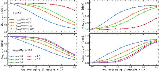
Measured scatter of the MS σ_{MS, 〈t〉} (left-hand panels) and offset from the intrinsic ridgeline Δ_{MS, 〈t〉} (right-hand panels) as a function of the averaging time-scale 〈t〉. Upper panels show the results for a power-law slope α = 2.0 and varying τ_break, while the lower panels show the results for a constant τ_break = 100.0 Myr and varying α. Averaging the SFHs of the model galaxies over longer time-scales increases the offset from the MS to higher values and leads to a decrease of the MS scatter, as already seen in Fig. 4.

Open in new tab Download slide

These plots confirm our intuitive findings from above. For a given indicator corresponding to a single averaging time-scale 〈t〉, the larger α and shorter τ_break leads to measuring a tighter MS and a larger offset from the median of the intrinsic MS.

Until now we have discussed how measurements (averaging in this simple toy case) and parameters of stochastic processes influence the statistical parameters of the final distribution such as median and standard deviation. In Fig. 6 we show a full example of the effect of averaging the SFR (i.e. measuring the SFR with a given indicator) on the observed MS. For all three panels we assume an averaging time-scale of 100 Myr and the slope α = 2, while varying the τ_break of the process. The blue points show the individual model galaxies. The dashed red line indicates the predicted connection between the measured and actual (intrinsic) offset from the MS according to equation (14). This prediction is in excellent agreement with the relation measured from simulated model galaxies, which is shown in orange. In the bottom right corner of each panel we also show the measured scatter of the MS and the predicted value from equation (16).

Figure 6.

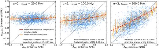
Distribution of measured offset from the main sequence as a function of intrinsic offset from the main sequence. ‘Measurement’ has been approximated in this simple example by averaging previous 100 Myr of SFH of each galaxy. From left to right, we show result for damped random walk with τ_break = 20, 100, and 500 Myr. The dashed diagonal line shows one-to-one relation. The orange line shows the mean Δ_ind,MS in the measured data, as a function of input Δ_MS, along with the 1-σ spread. The dashed red line shows our prediction for the mean Δ_ind,MS in the measured data, calculated from equation (14). In the bottom right corner we state measured scatter of the MS as seen in the simulated data, and from our analytical expression in equation (16). The small offset of the recovered parameters compared to input parameters is due to the fact that equation (16) is only the first-order approximation of the full expression.

Open in new tab Download slide

In the left-hand panel of Fig. 6, we can now explicitly see the central limit theorem in action: because the SFRs vary rapidly, the measured and intrinsic SFRs are almost completely unrelated. This is a consequence of the fact that the observational time-scale is much longer than the decorrelation time of the process. This means that during the time-scale of the observation, each galaxy has moved up and down the MS ridgeline and hence the measured SFR gives us only an estimate of the mean of the whole population. In the middle and right-hand panels of Fig. 6, we increase τ_break: the decorrelation times become longer and the agreement between the intrinsic and measured SFRs improve as galaxies change their SFRs less significantly during the time that measurement is sensitive to.

3.3 Measuring parameters of stochastic process from the mock data

In the previous section we have extensively discussed how averaging, i.e. measuring, SFRs changes the inferred properties of the MS, such as position of ridgeline and width. Furthermore, we have shown how this effect depends on the parameters of the stochastic process itself. Here we want to show how we can use these insights to deduce the parameters of the stochastic process from mock observations. We will then apply the same procedure, with more realistic response functions of different indicators, when discussing real data in Section 5.

Here we consider an example in which we have simulated 10 000 galaxies with α = 2 and τ_break = 400 Myr. We have then convolved these galaxies with three step functions of 1, 10, and 100 Myr respectively, mimicking three different indicators. Given that 1 Myr is the shortest time-scale that we consider, ‘measurement’ with the short indicator is the equivalent to the intrinsic SFH. We then measure the ratio of the widths of MS measured in each of these indicators, with associated error bars, and then find parts of the parameter space that are consistent with these measurements, both from considering equation (16) and from comparing with results from a simulation that spans the whole parameters space. We consider ratios of the measurements in different indicators to minimize the dependence of the result on the intrinsic width of the MS, which is of course known in the simulation, but is not necessarily available when considering real data. We see from equation (16), which is a first-order approximation to the actual measured width, that considering ratios of measured widths eliminates dependence on intrinsic σ_MS. Some dependence comes from higher order terms to equation (16), which we discuss in Appendix C.

We show the result of this procedure in Fig. 7. The dashed lines show the result deduced from analytic expression in equation (16) while the differently coloured areas show 1-σ constraints from the numerical simulations. We see that, although a single ratio of MS width measurements of two indicators is not sufficient to break the degeneracy between α and τ_break, combination of several indicators can break this degeneracy and provide a unique solution for the parameters of the process. This is not surprising, and is a restatement of the fact that we need two different ‘measurements’ in order to uniquely determine two free parameters. It is also advantageous if the indicators cover substantially different range of time-scales, in order to be sensitive to different parts of the PSD. Given that we aim to be as agnostic as possible to the intrinsic width of the MS and therefore consider ratios of the MS width, this effectively requires a measurement of the width of the MS with three indicators. Addition of any more indicators or combinations of indicators will not bring more information in this plane, but can be used as a consistency check.

Figure 7.

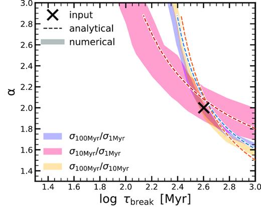
Example of recovering the parameters of a stochastic process by the MS width measurements. The black cross marks the input parameter for the simulated model galaxies (α = 2.0 and τ_break = 400 Myr). The dashed lines show the analytical constraints from the ratios of MS width measurements, while the shaded bands show the numerical constraints. The three different colours show the constraints for three different MS width measurements: a short, medium, and long time-scale indicator (1, 10, and 100 Myr). We find that we can recover the input parameters. The small offset of the analytically recovered parameters compared to input parameters is due to the fact that equation (16) is only the first-order approximation of the full expression.

Open in new tab Download slide

Furthermore, we see that there is a small offset from the input values and the values deduced from using equation (16). This is a consequence of the fact that equation (16) is only the first-order approximation to the full calculation of the width, as already discussed in Section 3.1.2 and Appendix C. We use full numerical simulations to avoid this effect here and when we compare with the real data in Section 5.

4 FINDING PARAMETERS OF STOCHASTIC STAR-FORMATION HISTORY WITH REALISTIC RESPONSE FUNCTIONS

We highlighted in the previous section that the MS scatter for the SFR average over different time-scales can give a tight constraint on the PSD of the underlying stochastic process. In this section, we present a detailed investigation quantifying how does the normalization and width of the MS change when probed with different SFR indicators, which themselves trace different time-scales. In Section 5, we will use this information to show example of constraining the PSD from observations.

4.1 SFR tracers

There are multiple methods for determining SFRs from observational tracers such as from the UV, IR, and emission lines. In the end, all the methods – irrespective of whether the observable is directly starlight, dust-reradiated starlight, or nebular line emission – quantitatively link the observable to the intrinsic emission from hot young stars. Therefore, a crucial part of each method deals with how to correct for dust attenuation. Similarly, the IMF, in particular the high-mass end slope, and the SFH play a role in the exact luminosity-SFR calibration.

In the scope of this work, we are primarily interested in the distribution of SFRs probed by different tracers and hence time-scales. We assume that measurements of dust-corrected SFRs as provided in the literature are accurately dust corrected, i.e. we do not discuss any dust effects. Similarly, we assume a Chabrier (2003) IMF and solar metallicity throughout. Variations in metallicity, dust attenuation (in particular differential dust effect between young and old stars) and IMF could be, in principle, important. We will address this in an upcoming publication, where we will study the effect of variability of SFHs, IMF, and dust attenuation in the observational plane of luminosities. In general, these effects would increase the scatter, implying that our results are basically an upper limit on the variability. In Section 5, we focus on a galaxy sample in a small mass range (M_⋆ = 10¹⁰–10^10.5M_⊙) in order to minimize variations in IMF, metallicity, and dust content.

We are considering the following standard SFR tracers (see Kennicutt 1998; Kennicutt & Evans 2012; Boquien et al. 2014; Davies et al. 2016):

H α: H α photons arise from the gas ionized by young (<20 Myr) stars. Thus, H α provides a measure of the current SFR in galaxies.
FUV and NUV: UV continuum emission arises from hot, massive O and B stars with M_⋆ > 3 M_⊙, and hence is a good tracer of more recent star formation, though on longer time-scales than H α.
u-band: The rest-frame u-band (∼3500 Å) emission arises from the photospheres of young, massive stars, tracing the star formation on |${\lesssim}100$| Myr time-scales. This emission is less strongly affected by dust obscuration than the UV, but the possible large contribution from older stellar populations makes it more difficult to interpret.
WISE W3: Probing infrared (IR) flux from star-forming galaxies in the 3–100 |$\mu$|m range gives a reliable estimate for the ongoing star-formation: the amount of flux emitted in the IR is directly related to the UV emission from newly formed stars (e.g. Calzetti et al. 2007). We consider the Wide-field Infrared Survey Explorer (WISE) passband W3 at rest-frame 12 |$\mu$|m to estimate the SFR (Cluver et al. 2014).
UV+IR: As discussed above, UV emission arises directly from star-forming regions, while some fraction of this emission is absorbed and reprocessed by dust, being re-emitted in the IR. We therefore sum both UV and total IR luminosities to obtain the total SFR, based on the bolometric luminosity of OB stars.

In order to now predict what the SFH, as seen by a certain indicator looks like, we need to convolve the intrinsic SFH with the response function of that indicator. Response functions for the aforementioned indicators are shown and discussed in Appendix D. Briefly, we predict the luminosity evolution for a Simple Stellar Population (SSP) using the Flexible Stellar Population Synthesis code (FSPS³; Conroy, Gunn & White 2009). FSPS has been extensively calibrated against a suite of observational data (for details see Conroy & Gunn 2010). Throughout this work, we adopt the MILES stellar library and the MIST isochrones. Since the W3 and UV+IR SFR tracers are based on emission from a large wavelength range, these indicators depend on the dust attenuation prescription. We assume a uniform screen with Cardelli, Clayton & Mathis (1989) attenuation curve and an opacity of τ = 0.5 at 5500 Å, motivated by findings by Salim, Boquien & Lee (2018) in the local universe. Changing this prescription does not affect our findings here significantly. As expected, and shown in Appendix D, the H α SFR indicator shows a rapid response function, followed by the FUV SFR indicator and the other indicators.

Fig. 8 shows the effect on the SFH by convolving the SFH with the response functions for the different indicators. In particular, the upper panel shows the distance from the MS, while the lower panel shows the absolute SFR under the assumption that the MS has an SFR of 1 M_⊙ yr⁻¹ at all times and masses. This SFH has PSD described with a high frequency power-law slope of α = 2 and a decorrelation time-scale of τ_break = 100 Myr.

Figure 8.

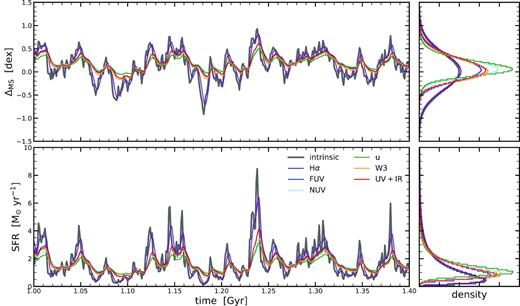
Example of the SFH of a galaxy as seen by different SFR indicators. The upper left-hand panel shows the distance from the MS as a function of time, while the bottom left-hand panel shows the absolute SFR, assuming the MS has a normalization of 1 M_⊙yr⁻¹ at all times and stellar masses. We show a small zoomed-in section from one of the simulated SFH, starting at 1 Gyr. The panels on the right show the 1d histograms of the projected SFR evolution. The intrinsic SFH is shown in black, while the purple, blue, cyan, green, orange, and red lines show the SFH as seen by the H α, FUV, NUV, u, W3, and UV+IR SFR indicators, respectively. Since H α probes short time-scales (see Fig. D1), it tracks the intrinsic SFH well. On the other hand, if the SFR indicator probes longer time-scales, the overall SFH is much smoother and there is an overall bias towards higher SFRs, leading to an offset of the inferred MS ridgeline.

Open in new tab Download slide

The SFR inferred from H α traces the intrinsic SFH well, only missing fluctuations on the shortest time-scale (∼4 Myr). All other tracers, which probe longer time-scales, show a much larger differences compared to the intrinsic SFH. We find that the SFHs are not only smoother, but because of the long time-scale tail in the response function, the SFRs are biased high. There is an overall mean offset of the MS. Additionally, we find that all the variability on short time-scales (<20 Myr) are washed out, giving rise to a narrower MS width. This is overall consistent with the simple analysis presented in the previous section.

4.2 Shape of the MS as seen by different SFR indicators: normalization and scatter

We go now one step further and look how the effect on the MS depends on the PSD itself. Fig. 9 is a remake of Fig. 4, showing the distribution of the distances from the MS ridgeline for different SFR indicators. We see the same qualitative behaviour that we discussed extensively in Fig. 4, when we discussed the simplified case in which we simply averaged SFRs over a certain time-scale. Measurements in H α, which probe star-formation on the shortest time-scale, follows the intrinsic distribution closely for all but the most ‘bursty’ set of parameters. On the other hand, all other indicators show some level of deviation, and produce a narrower distribution that is offset from the intrinsic value of the MS. Indicators that act on longer time-scales tend to produce narrower distributions, which is in very good agreement with observations (e.g. fig. 7 from Davies et al. 2019). The differences in the shapes, even if not so pronounced as in the simple case shown in Fig. 4, can be again used to infer the intrinsic properties of the underlying stochastic process.

Figure 9.

Distribution about the MS ridgeline as seen by different SFR indicators. This figure is similar to Fig. 4, but this time for realistic SFR indicators. Each panel shows the resulting distributions for a given PSD, with increasing α and τ_break from top left to bottom right. The thick black histogram indicates the intrinsic distribution, which has by construction a mean of 0.0 and a scatter of 0.4 dex for all α and τ_break. The purple, blue, cyan, green, orange, and red histograms show the distribution of galaxies as seen by the H α, FUV, NUV, u, W3, and UV+IR SFR indicator, respectively. The larger the time-scale probed by the indicator, the larger the MS offset and the smaller the MS scatter. The effects are the largest for small α and τ_break since the PSD has a lot of power on short time-scales relative to the long time-scales.

Open in new tab Download slide

Although both the normalization as well as the width of the MS as seen by different indicators can in principle be used to derive the PSD, we are focusing now on the width of the MS. We do this because the overall normalization depends on the exact conversion used to derive SFRs from fluxes, which are uncertain and depend on several assumption like the IMF, metallicity, as well as the assumed SFH. On the other hand, the width of the MS is a relative measure that depends only on the rank-ordering in the galaxy sample and as such it is largely independent on the exact flux-SFR conversion.

Fig. 10 shows how the scatter of the MS changes when traced by different SFR indicators. This figure assumes that the intrinsic width of the MS is 0.4 dex (probed on a 1 Myr time-scale). Specifically, each panel shows the MS scatter as a function of the PSD parameters α and τ_break. We see a similar pattern that we have also seen when we have discussed ‘burstiness’ (Fig. 3). Consistent with the previous figure, measurements in H α follow the intrinsic width closely for large parts of the parameter space. Measurements in other indicators that depend more heavily on the previous SFH provide a measurement that is less readily interpretable. In general, as discussed in Section 2, processes with low α and τ_break that oscillate wildly, lead to tighter observed MS, courtesy of the central limit theorem. Although measured width in different indicators are relatively similar, the differences between them enable us to constraint parameters of the underlying process in Section 5.

Figure 10.

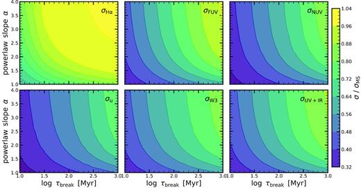
The scatter of the MS as seen by different indicators. Each panel shows the MS scatter as seen by a certain indicator as a function of the PSD parameters τ_break and α. The panels from the top left to the bottom right show the results for the H α, FUV, NUV, u, W3, and UV+IR SFR indicator. In general, the burstier the SFR (see Fig. 3), the smaller the measured scatter with the indicator.

Open in new tab Download slide

4.3 Ratio of SFRs with different indicators

We now move forward to an MS-independent discussion and directly compare different SFR tracers with each other in Fig. 11. Specifically, we plot the ratio of FUV and H α SFRs versus the ratio of u-band and H α SFRs. The colour-coding corresponds to the ratio of the SFR measured over 1 Myr and the SFR measured over 100 Myr. There are three trends visible from this figure. Firstly, the tightness of the relation increases with increasing burstiness. This arises because all SFR indicators probe the same SFR if the SFR varies on shorter time-scales than the time-scales of the SFR indicators. Second, the slope decreases with decreasing burstiness. This can be explained by the fact that the H α and FUV SFR indicators are able to probe short-term variability better than the u-band SFR indicator, which, in the case of slowly varying SFHs, leads to a FUV-to-H α ratio close to 1 while the u-band-to-H α ratio shows significantly more scatter. Thirdly, the colour-coding shows that if the SFH quickly increases, H α is able to probe this, leading to ratios smaller than 1, while if the SFH quickly decreases, the ratios are all larger than 1. Overall, this figure highlights that – in the framework presented in this work – there are quantifiable consequences that arise when simply investigating the relation between the SFR measured with different indicators.

Figure 11.

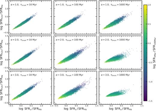
The distribution of galaxies in the plane of SFR_FUV/SFR_H α versus SFR_u/SFR_H α. Each panel shows the resulting distributions for a given PSD, with increasing α and τ_break from top left to bottom right. The colour-coding corresponds to the ratio of the SFR measured over 1 Myr and the SFR measured over 100 Myr. The shapes of these distributions differ – highlighting the possibility to constrain the PSD with such observations.

Open in new tab Download slide

5 OBSERVATIONAL CONSTRAINTS

In this section, we wish to apply our insights about different stochastic processes and their influence on observed MS properties. The main goal is to use the MS width measurements to determine parameters of the stochastic process, i.e. slope α and decorrelation time-scale τ_break of the PSD, that govern the evolution of star-forming galaxies about the MS ridgeline. The analysis in this section should be regarded only as a proof of concept as we work with the simplest possible assumptions, in order to highlight the power of our approach. We show that the result for the parameters that we derive are consistent when using different indicators, which is highly encouraging.

5.1 Main result

The ideal data set should contain statistically significant sample of galaxies and be covered in a several observational bands, in order to check consistency between different SFR indicators. Additionally, the analysis is simplified in the case of a galaxy sample at low redshift. This is because of (i) the slow evolution of the MS as a function of time, which simplifies interpretation of measured SFRs as an offset from the virtually non-changing MS; and (ii) the slow growth of mass, meaning that measurement of total stellar mass and star-formation are independent quantities. We discuss these issues more in Section 5.2. Additionally, low redshift sample also avoids potential problems and systematics that might arise due to K-correction.

We find the measurement of the MS width presented in Davies et al. (2019) to be well suited for this analysis. Davies et al. (2019) used data from Galaxy and Mass Assembly Survey (GAMA; Driver et al. 2011; Liske et al. 2015; Driver et al. 2016; Baldry et al. 2018) and conducted an analysis that was explicitly measuring width of the MS with different SFR indicators. The sample consists of 9005 galaxies and is restricted to z < 0.1, satisfying our requirement to work with a large sample at low redshift. It includes only galaxies that are not classified as being a member of a group or a pair in the GAMA group catalogue, as described in Robotham & Driver (2011). This means that our final result will be more suited to describing star-formation fluctuations due to ‘secular’ evolution instead of mergers.

We consider the following measurements: (i) extinction-corrected H α SFRs, measured with the process outlined in Gunawardhana et al. (2011), Hopkins et al. (2013), Gunawardhana et al. (2015) and using line measurements from Gordon et al. (2017), (ii) UV+IR SFRs, derived from the galaxy spectra as described in Brown et al. (2014), and (iii) extinction-corrected u-band SFRs from rest-frame u-band luminosity Davies et al. (2016). SFRs have been derived using Chabrier IMF. The MS width reported in Davies et al. (2019) is defined as the standard deviation of the sSFR values in a given stellar mass bin for all star-forming galaxies, i.e. no particular parametrization for the MS has been used. Star-forming galaxies are defined by a cut in sSFR. In order to derive the intrinsic scatter of the MS, we have deconvolved the observed MS scatter by the error estimates of each SFR indicator: |$\sigma _{\rm ind}=\sqrt{(\sigma _{\rm obs}^2-\sigma _{\rm err}^2)}$|⁠. We have taken error estimates of each SFR indicator from Davies et al. (2016): (σ_err(H α), σ_err(u), σ_err(UV + IR)) = (0.07, 0.03, 0.07) dex. We refer the reader to Davies et al. (2019) for more details.

We consider MS width measurements for SFR selected galaxies between 10^10.0 and 10^10.5M_⊙ as we expect that the measurement errors are the smallest for this subset of galaxies. Furthermore, more massive galaxies are transitioning from the star-forming to the quiescent population (quenching, e.g. Peng et al. 2010), which could lead to an artificially large scatter of the MS, which itself would depend heavily on the selection of star-forming galaxies. We estimate, using equation (27) from Peng et al. (2010) with reasonable quenching time of 1 Gyr, that only around 2|${{\ \rm per\ cent}}$| of star-forming galaxies at this mass are being ‘quenched’ at redshift 0. Additionally, considering the rather narrow mass range makes our result less affected by possible variations of dust and IMF within the sample.

The final result for our fiducial mass bin log (M_⋆/M_⊙) = 10.0–10.5 is shown in Fig. 12. As elaborated in Section 3, we consider ratios of the MS widths measured with different indicators to reduce the influence of the unknown intrinsic width of the MS on our measurement. As indicated beforehand, this analysis assumed intrinsic σ_MS = 0.4 dex, motivated by measured values in Davies et al. (2019). For interested readers, we show in Appendix B2 the effect of the large changes to the assumed intrinsic σ_MS on the final result.

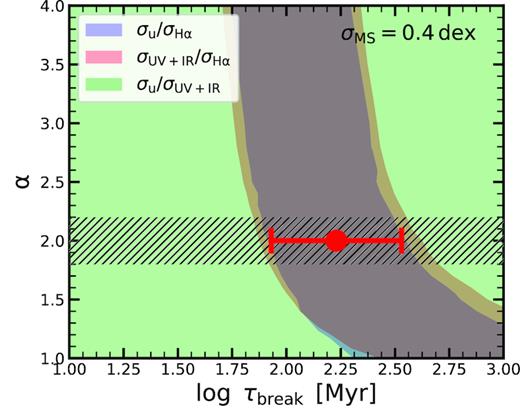
$Observational constraints on the PSD. We plot current observational constraints from the width of the MS in the plane of α and τbreak. Specifically, the blue, red, and green shaded regions show the constraints obtained from the ratio of the width of the MS as measured using the u-band and H α, UV+IR, and H α, and u-band and UV+IR, respectively. The overlapping region gives a tighter constraint in τbreak than α. Assuming α = 2 and σMS = 0.4 dex, we obtain $\tau _{\rm break}=170^{+169}_{-85}~\mathrm{Myr}$, which is indicated by the horizontal red errorbar.$

Figure 12.

Observational constraints on the PSD. We plot current observational constraints from the width of the MS in the plane of α and τ_break. Specifically, the blue, red, and green shaded regions show the constraints obtained from the ratio of the width of the MS as measured using the u-band and H α, UV+IR, and H α, and u-band and UV+IR, respectively. The overlapping region gives a tighter constraint in τ_break than α. Assuming α = 2 and σ_MS = 0.4 dex, we obtain |$\tau _{\rm break}=170^{+169}_{-85}~\mathrm{Myr}$|⁠, which is indicated by the horizontal red errorbar.

Open in new tab Download slide

The shaded regions in Fig. 12 correspond to the region where the measured and the modelled ratio of σ_{MS, ind} are within 10 per cent of each other. We have decided to use this value of 10 per cent to report the result in this work as the formal statistical errors on the measurements of the width of the MS are minute, given the larger number of objects considered in Davis et al. (2019) (e.g. consider fig. 4 in Davis et al. 2019). We believe that systematic effects, such as the aperture correction, the dust attenuation correction, and the changes to IMF and metallicity are likely to be main drivers of the error. It is beyond the scope of this paper to assess the impact of those uncertainties in detail, but all of these should contribute to relatively large error that we have assumed here.

We see the similar structure as in Fig. 7, with the general degeneracy between α and τ_break. We find the consistency between all of the indicators very encouraging, especially given the simplicity of our assumptions and minimal consideration of the dust and IMF effects. We see that σ_u/σ_{UV + IR} combination, although consistent with other combination, does not add constraining power to this result. This is due to similarity of the results coming out of |$\sigma _{\rm u}/\sigma _{\rm H_{\rm \alpha }}$| and |$\sigma _{\rm UV{+}IR}/\sigma _{\rm H_{\rm \alpha }}$| combinations. Interested reader may consult Appendix B2 for an example in which all combination contribute to the final result.

Unfortunately, with this data and simplicity of our analysis it is not possible to resolve the degeneracy between α and τ_break, as it has been possible in the simplified case considered in Section 3.2. This is due to combination of two factors. First, this is due to larger uncertainties in the observational measurement of the σ_MS, driven by the smaller number of galaxies in the sample and by the observational uncertainties. Secondly, the fact that realistic indicators are not a simple step functions but have non-trivial time dependence that mixes many time-scales reduces our ability to differentiate between the influence of α and τ_break in observations (see Fig. 10 and Appendix D).

In order to quantify our final result in one number, we report τ_break after setting the high-frequency slope at α = 2, i.e. for the case of damped random walk. We emphasize however that the data itself does not prefer α = 2 over any other particular value for α and our choice for reporting τ_break for damped random walk is driven by theoretical and empirical reasons outside of the scope of this paper. The first reason for considering the damped random walk is its theoretical and physical simplicity. Secondly, the slope of α = 2 is seen when studying time-variability properties of galaxies in simulations (Iyer et al., in preparation). In the case of α = 2, we find that the region of the τ_break parameter space that is within 1-σ contours for all combinations of indicators is given with |$\tau _{\rm break}=170^{+169}_{-85}$| Myr. We intentionally do not conduct further statistical consideration of the allowed region, given that we believe that systematic uncertainties, due to variation of dust, IMF, and observational uncertainties dominate our error budget and would make any such analysis highly uncertain. We do note that measurement of the width of MS by other indicators available in Davies et al. (2019) are in broad agreement with the estimated value that is reported above.

5.2 Discussion

5.2.1 Mass dependence

The result of |$\tau _{\rm break}=170^{+169}_{-85}~\mathrm{Myr}$| that we have derived is only valid for the sample that we considered, consisting of isolated galaxies with log (M_⋆/M_⊙) = 10.0–10.5. As such, the derived time-scale is not necessarily the same for the whole range of masses and environments in the Universe. We do note that there is a mass dependence in the measurements of the width of the MS in Davies et al. (2019). We do not conduct the mass dependence analysis in this work given the possible mass dependence in the dust and IMF properties. We do however note that the measured widths of the MS suggest similar or somewhat shorter time-scale for τ_break for the smaller masses within the data set (8 < log (M/M_⊙) < 10), with some dependence on the exact set of indicators used.

5.2.2 Caveats

Of course, our analysis comes with several caveats. One complication that we consider is the intrinsic correlation between the stellar mass and measured SFR. As we have elaborated, the measured SFR can be considered as an imperfect averaging over the intrinsic SFR, where the length of this averaging is dependent on the indicator used for the measurement. On the other hand, the stellar mass of a galaxy is also obviously related with the previous SFR, given by the integral over the complete SFH of the galaxy. Hence, the measurement of the MS width is only meaningful if the total stellar mass added over the period that a given indicator is measuring is small compared to the total stellar mass of a galaxy. Given that the mass doubling time for star-forming galaxies today is very long, i.e. comparable to Hubble time, the mass added over the time effectively probed by the different indicators is negligible (see also Appendix E). This effect, however, needs to be accounted for at higher redshifts (e.g. z > 1) where the time-scale of the measurement of star-formation in slow-response indicators starts being a non-negligible fraction of the lifetime of the Universe (e.g. Tacchella et al. 2018).

Similarly, when conducting our analysis of observational results we have assumed that the overall change of the mean SFR of the MS is negligible. Consider the time-scale of 400 Myr, which is more than twice as long as the τ_break derived above. We show in Appendix D that by this time-scale all of the considered indicators have outputted more than 60 per cent of their complete luminosity, i.e. are very weakly sensitive to the star-formation on longer time-scales. If we assume relatively steep evolution of the sSFR of the MS, such as (1 + z)³ (e.g. Lilly et al. 2013, and references therein), we find that the ratio between sSFR_MS(400 Myr)/sSFR_MS(today) ≈ 1.1. As such this change will have minimal effect on the inferred result in this study, but it needs to be considered at higher redshifts. Further discussion of a similar effect, where we superimpose global log-normal evolution to the stochastic SFH of the galaxies, can be found in Appendix B1.

6 SUMMARY AND CONCLUSIONS

The knowledge of how the SFR changes as a function of time for individual galaxies is a critical ingredient needed for understanding the evolution of galaxies. SFHs encode information about the variability on short and long time-scales that arise from different physical processes, such as gas accretion, mergers, and feedback from stars and black holes. The best method to model, and mathematically describe, SFHs is still being debated.

In this paper, we present a framework for modelling SFHs of galaxies as a stochastic process. We focus on star-forming galaxies and assume that a stochastic process describes how these galaxies move about the MS ridgeline. We also assume that at any moment the intrinsic distribution of SFRs around the MS ridgeline is log-normal. We define this stochastic process through a PSD. The functional form of the PSD is given by a broken power law, with high-frequency slope α that flattens out at a frequency corresponding to τ_break. The physical meaning of the PSD is that SFHs are correlated on short time-scales, where the strength of this correlation is described by the slope α, and they decorrelate to resemble white noise at a time-scale that is proportional to τ_break. Specifically, when the slope of the PSD is shallow and/or τ_break is small, the SFH violently oscillates around the mean and is very quickly decorrelated. On the other hand, steeper slopes and longer τ_break lead to slower oscillations and a more correlated behaviour.

We demonstrate that, even though we cannot observationally follow the time-evolution of individual galaxies, we can deduce the properties of the stochastic process. This can be done by measuring properties of the MS, such as the MS normalization and the MS scatter, with different observational indicators that are sensitive to different time-scales. There exists a degree of degeneracy between the influence of the parameters α and τ_break, that can be roughly described by the ‘burstiness’, i.e. by the fact that galaxies described with smaller α and shorter τ_break tend to more often have SFRs which are outside of the 1-σ width of the MS. We show that this degeneracy can be broken, in principle, by measuring the properties of the MS in several observational indicators.

We then consider realistic observational SFR indicators, and show results for the measured properties of the MS in H α, FUV, NUV, u-, W3, and UV+IR bands. We use those results to, as a proof of concept, deduce parameters of the underlying stochastic process from the data from the GAMA survey, presented in Davies et al. (2019). For a sample of isolated galaxies with log (M_⋆/M_⊙) = 10.0–10.5 and using MS widths measured from H α, u- and UV+IR bands, we find the area of the parameter space that is consistent with this data. With an assumption that the high-frequency slope is given with α = 2, we obtain |$\tau _{\rm break}=170^{+169}_{-85}~\mathrm{Myr}$|⁠. The motivation for α = 2 stems from numerical simulations as well as the theoretical attractiveness of the damped random walk process. The quoted errobars are deduced from the observational 1-σ errors of all the available indicators.

Our result of τ_break ≈ 200 Myr indicates that the SFHs of galaxies decorrelate, i.e. lose memory of their previous SFH, on roughly this time-scale. This is shorter than the dynamical time of the dark matter halo, which is roughly 10 per cent of the Hubble time (i.e. a bit more than a Gyr at z ∼ 0). Therefore, we conclude that baryonic effects within the haloes, which act on dynamical time-scales of galaxies, play an important role in shaping the SFHs of galaxies. Examples of such effects could include feedback and reincorporation of galactic winds.

In the future, we will apply this framework to a wide range of numerical and semi-analytical models, where we can measure the PSD directly of the models’ SFHs. Preliminary results show that the obtained PSDs are well described by a broken power law with nearly all theoretical models producing α ≈ 2, while having different values for τ_break. We show that the PSD is set by physical ingredients in the models and hence that the PSD contains a wealth of information that has not yet been researched. On the observational side, we will address many issues that complicate precise determination of the PSD in observations, including possible variations in the IMF and dust attenuation. There we also wish to use these insights to analyse properties of galaxies at higher redshifts, where it is especially important to consider these complications.

ACKNOWLEDGEMENTS

We thank the referee, Kartheik Iyer, for a constructive report and useful comments. We thank Luke Davis for sharing his measurements from the GAMA survey with us. Furthermore, we are thankful to Charlie Conroy, Luke Davis, Daniel Eisenstein, Ben Johnson, Daniel Kelson, Joel Leja, Chelsea MacLeod, and Michael Strauss for very useful comments. We thank Sophie Reed and Hassan Siddiqui for proofreading the manuscript. This research made use of NASA’s Astrophysics Data System (ADS), the arXiv.org preprint server, the Python plotting library matplotlib (Hunter 2007), astropy, a community-developed core Python package for Astronomy (Astropy Collaboration 2013), and the python binding of FSPS (Foreman-Mackey, Sick & Johnson 2014). ST is supported by the Smithsonian Astrophysical Observatory through the CfA Fellowship.

Footnotes

1

In the rest of the paper α will appear as a positively defined quantity, i.e. α is defined with equation (5), and not with PSD(f) ∝ f^α.

2

We henceforth use just Δ as shorthand for Δ_MS in equations, in order to reduce the size and complexity of our expressions.

3

https://github.com/cconroy20/fsps

4

Here we discuss ‘type 2’ fractional Brownian motion, which is more suited for descriptions of physical process as in that description the future events are only dependent on the previous events. ‘Type 1’ processes are dependent on both future and past events, violating causality.

5

As mentioned in the main body of the text, we use just Δ as shorthand for Δ_MS in order to reduce the size and complexity of our expressions.

REFERENCES

Abramson

L. E.

et al. .,

2018

,

AJ

,

156

,

29

10.3847/1538-3881/aac822

Crossref

Search ADS

Abramson

L. E.

,

Gladders

M. D.

,

Dressler

A.

,

Oemler

A.

Jr,

Poggianti

B.

,

Vulcani

B.

,

2015

,

ApJ

,

801

,

L12

10.1088/2041-8205/801/1/L12

Crossref

Search ADS

Applebaum

E.

,

Brooks

A. M.

,

Quinn

T. R.

,

Christensen

C. R.

,

2018

, preprint (arXiv:1811.00022)

Astropy Collaboration

,

2013

,

A&A

,

558

,

A33

10.1051/0004-6361/201322068

Crossref

Search ADS

Baldry

I. K.

,

Glazebrook

K.

,

Brinkmann

J.

,

Ivezić

Ž.

,

Lupton

R. H.

,

Nichol

R. C.

,

Szalay

A. S.

,

2004

,

ApJ

,

600

,

681

10.1086/380092

Crossref

Search ADS

Baldry

I. K.

et al. .,

2018

,

MNRAS

,

474

,

3875

10.1093/mnras/stx3042

Crossref

Search ADS

Barro

G.

et al. .,

2017

,

ApJ

,

840

,

47

10.3847/1538-4357/aa6b05

Crossref

Search ADS

Behroozi

P. S.

,

Wechsler

R. H.

,

Conroy

C.

,

2013

,

ApJ

,

770

,

57

10.1088/0004-637X/770/1/57

Crossref

Search ADS

Boogaard

L. A.

et al. .,

2018

,

A&A

,

619

,

A27

10.1051/0004-6361/201833136

Crossref

Search ADS

Boquien

M.

,

Buat

V.

,

Perret

V.

,

2014

,

A&A

,

571

,

A72

10.1051/0004-6361/201424441

Crossref

Search ADS

Bouché

N.

et al. .,

2010

,

ApJ

,

718

,

1001

10.1088/0004-637X/718/2/1001

Crossref

Search ADS

Brinchmann

J.

,

Charlot

S.

,

White

S. D. M.

,

Tremonti

C.

,

Kauffmann

G.

,

Heckman

T.

,

Brinkmann

J.

,

2004

,

MNRAS

,

351

,

1151

10.1111/j.1365-2966.2004.07881.x

Crossref

Search ADS

Broussard

A.

et al. .,

2019

,

ApJ

,

873

,

74

10.3847/1538-4357/ab04ad

Crossref

Search ADS

Brown

M. J. I.

et al. .,

2014

,

ApJS

,

212

,

18

10.1088/0067-0049/212/2/18

Crossref

Search ADS

Calzetti

D.

et al. .,

2007

,

ApJ

,

666

,

870

10.1086/520082

Crossref

Search ADS

Caplar

N.

,

Lilly

S. J.

,

Trakhtenbrot

B.

,

2015

,

ApJ

,

811

,

148

10.1088/0004-637X/811/2/148

Crossref

Search ADS

Caplar

N.

,

Lilly

S. J.

,

Trakhtenbrot

B.

,

2017

,

ApJ

,

834

,

111

10.3847/1538-4357/834/2/111

Crossref

Search ADS

Caplar

N.

,

Lilly

S. J.

,

Trakhtenbrot

B.

,

2018

,

ApJ

,

867

,

148

10.3847/1538-4357/aae691

Crossref

Search ADS

Cardelli

J. A.

,

Clayton

G. C.

,

Mathis

J. S.

,

1989

,

ApJ

,

345

,

245

10.1086/167900

Crossref

Search ADS

Carnall

A. C.

,

Leja

J.

,

Johnson

B. D.

,

McLure

R. J.

,

Dunlop

J. S.

,

Conroy

C.

,

2019

,

ApJ

,

873

,

44

10.3847/1538-4357/ab04a2

Crossref

Search ADS

Carollo

C. M.

et al. .,

2013

,

ApJ

,

773

,

112

10.1088/0004-637X/773/2/112

Crossref

Search ADS

Ceverino

D.

,

Klypin

A.

,

Klimek

E. S.

,

Trujillo-Gomez

S.

,

Churchill

C. W.

,

Primack

J.

,

Dekel

A.

,

2014

,

MNRAS

,

442

,

1545

10.1093/mnras/stu956

Crossref

Search ADS

Chabrier

G.

,

2003

,

PASP

,

115

,

763

10.1086/376392

Crossref

Search ADS

Chang

Y.-Y.

,

van der Wel

A.

,

da Cunha

E.

,

Rix

H.-W.

,

2015

,

ApJS

,

219

,

8

10.1088/0067-0049/219/1/8

Crossref

Search ADS

Cluver

M. E.

et al. .,

2014

,

ApJ

,

782

,

90

10.1088/0004-637X/782/2/90

Crossref

Search ADS

Connolly

S.

,

2015

, preprint (arXiv:1503.06676)

Conroy

C.

,

2013

,

ARA&A

,

51

,

393

10.1146/annurev-astro-082812-141017

Crossref

Search ADS

Conroy

C.

,

Gunn

J. E.

,

2010

,

ApJ

,

712

,

833

10.1088/0004-637X/712/2/833

Crossref

Search ADS

Conroy

C.

,

Gunn

J. E.

,

White

M.

,

2009

,

ApJ

,

699

,

486

10.1088/0004-637X/699/1/486

Crossref

Search ADS

Daddi

E.

et al. .,

2007

,

ApJ

,

670

,

156

10.1086/521818

Crossref

Search ADS

Daddi

E.

et al. .,

2010

,

ApJ

,

713

,

686

10.1088/0004-637X/713/1/686

Crossref

Search ADS

Damjanov

I.

,

Hwang

H. S.

,

Geller

M. J.

,

Chilingarian

I.

,

2014

,

ApJ

,

793

,

39

10.1088/0004-637X/793/1/39

Crossref

Search ADS

Damjanov

I.

,

Zahid

H. J.

,

Geller

M. J.

,

Utsumi

Y.

,

Sohn

J.

,

Souchereau

H.

,

2019

,

ApJ

,

872

,

91

10.3847/1538-4357/aaf97d

Crossref

Search ADS

Davé

R.

,

Finlator

K.

,

Oppenheimer

B. D.

,

2012

,

MNRAS

,

421

,

98

10.1111/j.1365-2966.2011.20148.x

Crossref

Davies

L. J. M.

et al. .,

2015

,

MNRAS

,

452

,

616

10.1093/mnras/stv1241

Crossref

Search ADS

Davies

L. J. M.

et al. .,

2016

,

MNRAS

,

461

,

458

10.1093/mnras/stw1342

Crossref

Search ADS

Davies

L. J. M.

et al. .,

2019

,

MNRAS

,

483

,

1881

10.1093/mnras/sty2957

Crossref

Search ADS

Davis

T. A.

,

van de Voort

F.

,

Rowlands

K.

,

McAlpine

S.

,

Wild

V.

,

Crain

R. A.

,

2019

,

MNRAS

,

484

,

2447

10.1093/mnras/stz180

Crossref

Search ADS

Dekel

A.

,

Mandelker

N.

,

2014

,

MNRAS

,

444

,

2071

10.1093/mnras/stu1427

Crossref

Search ADS

Dexter

J.

,

Agol

E.

,

2011

,

ApJ

,

727

,

L24

10.1088/2041-8205/727/1/L24

Crossref

Search ADS

Djorgovski

S.

,

Davis

M.

,

1987

,

ApJ

,

313

,

59

10.1086/164948

Crossref

Search ADS

Driver

S. P.

et al. .,

2011

,

MNRAS

,

413

,

971

10.1111/j.1365-2966.2010.18188.x

Crossref

Search ADS

Driver

S. P.

et al. .,

2016

,

MNRAS

,

455

,

3911

10.1093/mnras/stv2505

Crossref

Search ADS

Eales

S.

,

de Vis

P.

,

W. L. Smith

M.

,

Appah

K.

,

Ciesla

L.

,

Duffield

C.

,

Schofield

S.

,

2017

,

MNRAS

,

465

,

3125

10.1093/mnras/stw2875

Crossref

Search ADS

Elbaz

D.

et al. .,

2007

,

A&A

,

468

,

33

10.1051/0004-6361:20077525

Crossref

Search ADS

Emami

N.

,

Siana

B.

,

Weisz

D. R.

,

Johnson

B. D.

,

Xiancheng

M.

,

Kareem

E.

,

2018

, preprint (arXiv:1809.06380)

Emmanoulopoulos

D.

,

McHardy

I. M.

,

Uttley

P.

,

2010

,

MNRAS

,

404

,

931

10.1111/j.1365-2966.2010.16328.x

Crossref

Search ADS

Emmanoulopoulos

D.

,

McHardy

I. M.

,

Papadakis

I. E.

,

2013

,

MNRAS

,

433

,

907

10.1093/mnras/stt764

Crossref

Search ADS

Faber

S. M.

,

Jackson

R. E.

,

1976

,

ApJ

,

204

,

668

10.1086/154215

Crossref

Search ADS

Fagioli

M.

,

Carollo

C. M.

,

Renzini

A.

,

Lilly

S. J.

,

Onodera

M.

,

Tacchella

S.

,

2016

,

ApJ

,

831

,

173

10.3847/0004-637X/831/2/173

Crossref

Search ADS

Faucher-Giguère

C.-A.

,

2018

,

MNRAS

,

473

,

3717

10.1093/mnras/stx2595

Crossref

Search ADS

Feldmann

R.

,

2017

,

MNRAS

,

470

,

L59

10.1093/mnrasl/slx073

Crossref

Search ADS

Foreman-Mackey

D.

,

Sick

J.

,

Johnson

B.

,

2014

,

Python-fsps: Python bindings to FSPS v0.1.1

,

Zenodo

.

10.5281/zenodo.12157

Google Scholar

Google Preview

OpenURL Placeholder Text

WorldCat

Crossref

Freeman

P.

,

Rosolowsky

E.

,

Kruijssen

J. M. D.

,

Bastian

N.

,

Adamo

A.

,

2017

,

MNRAS

,

468

,

1769

10.1093/mnras/stx499

Crossref

Search ADS

Genzel

R.

et al. .,

2010

,

MNRAS

,

407

,

2091

10.1111/j.1365-2966.2010.16969.x

Crossref

Search ADS

Genzel

R.

et al. .,

2015

,

ApJ

,

800

,

20

10.1088/0004-637X/800/1/20

Crossref

Search ADS

Gladders

M. D.

,

Oemler

A.

,

Dressler

A.

,

Poggianti

B.

,

Vulcani

B.

,

Abramson

L.

,

2013

,

ApJ

,

770

,

64

10.1088/0004-637X/770/1/64

Crossref

Search ADS

Goh

K.-I.

,

Barabási

A.-L.

,

2008

,

Europhys. Lett.

,

81

,

48002

10.1209/0295-5075/81/48002

Crossref

Search ADS

Gordon

Y. A.

et al. .,

2017

,

MNRAS

,

465

,

2671

10.1093/mnras/stw2925

Crossref

Search ADS

Graves

G. J.

,

Schiavon

R. P.

,

2008

,

ApJS

,

177

,

446

10.1086/588097

Crossref

Search ADS

Grudić

M. Y.

,

Hopkins

P. F.

,

Faucher-Giguère

C.-A.

,

Quataert

E.

,

Murray

N.

,

Kereš

D.

,

2018

,

MNRAS

,

475

,

3511

10.1093/mnras/sty035

Crossref

Search ADS

Gunawardhana

M. L. P.

et al. .,

2011

,

MNRAS

,

415

,

1647

10.1111/j.1365-2966.2011.18800.x

Crossref

Search ADS

Gunawardhana

M. L. P.

et al. .,

2015

,

MNRAS

,

447

,

875

10.1093/mnras/stu2232

Crossref

Search ADS

Guo

Y.

et al. .,

2016

,

ApJ

,

833

,

37

10.3847/1538-4357/833/1/37

Crossref

Search ADS

Guo

K.

,

Zheng

X. Z.

,

Fu

H.

,

2013

,

ApJ

,

778

,

23

10.1088/0004-637X/778/1/23

Crossref

Search ADS

Henriques

B. M. B.

,

White

S. D. M.

,

Thomas

P. A.

,

Angulo

R.

,

Guo

Q.

,

Lemson

G.

,

Springel

V.

,

Overzier

R.

,

2015

,

MNRAS

,

451

,

2663

10.1093/mnras/stv705

Crossref

Search ADS

Hollyhead

K.

,

Bastian

N.

,

Adamo

A.

,

Silva-Villa

E.

,

Dale

J.

,

Ryon

J. E.

,

Gazak

Z.

,

2015

,

MNRAS

,

449

,

1106

10.1093/mnras/stv331

Crossref

Search ADS

Hopkins

P. F.

,

Kereš

D.

,

Oñorbe

J.

,

Faucher-Giguère

C.-A.

,

Quataert

E.

,

Murray

N.

,

Bullock

J. S.

,

2014

,

MNRAS

,

445

,

581

10.1093/mnras/stu1738

Crossref

Search ADS

Hopkins

A. M.

et al. .,

2013

,

MNRAS

,

430

,

2047

10.1093/mnras/stt030

Crossref

Search ADS

Hunter

J. D.

,

2007

,

Comput. Sci. Eng.

,

9

,

90

Crossref

Search ADS

Ivezić

,

Ž.

,

Connolly

A. J.

,

Vanderplas

J. T.

,

Gray

A.

,

2014

,

Statistics, Data Mining and Machine Learning in Astronomy

.

Princeton Univ. Press

,

Princeton

Google Scholar

Google Preview

OpenURL Placeholder Text

WorldCat

Iyer

K.

,

Gawiser

E.

,

2017

,

ApJ

,

838

,

127

10.3847/1538-4357/aa63f0

Crossref

Search ADS

Iyer

K.

et al. .,

2018

,

ApJ

,

866

,

120

10.3847/1538-4357/aae0fa

Crossref

Search ADS

Johnson

B. D.

et al. .,

2013

,

ApJ

,

772

,

8

10.1088/0004-637X/772/1/8

Crossref

Search ADS

Katsianis

A.

,

2019

,

ApJ

,

preprint (

arXiv:1905.02023)

Kelly

B. C.

,

Bechtold

J.

,

Siemiginowska

A.

,

2009

,

ApJ

,

698

,

895

10.1088/0004-637X/698/1/895

Crossref

Search ADS

Kelly

B. C.

,

Becker

A. C.

,

Sobolewska

M.

,

Siemiginowska

A.

,

Uttley

P.

,

2014

,

ApJ

,

788

,

33

10.1088/0004-637X/788/1/33

Crossref

Search ADS

Kelson

D. D.

,

2014

, preprint (arXiv:1406.5191)

Kelson

D. D.

,

Benson

A. J.

,

Abramson

L. E.

,

2016

, preprint (arXiv:1610.06566)

Kennicutt

R. C.

Jr,

1998

,

ARA&A

,

36

,

189

10.1146/annurev.astro.36.1.189

Crossref

Search ADS

Kennicutt

R. C.

,

Evans

N. J.

,

2012

,

ARA&A

,

50

,

531

10.1146/annurev-astro-081811-125610

Crossref

Search ADS

Kormendy

J.

,

1977

,

ApJ

,

218

,

333

10.1086/155687

Crossref

Search ADS

Kruijssen

J. M. D.

,

Longmore

S. N.

,

2014

,

MNRAS

,

439

,

3239

10.1093/mnras/stu098

Crossref

Search ADS

Kruijssen

J. M. D.

,

Schruba

A.

,

Hygate

A. P. S.

,

Hu

C.-Y.

,

Haydon

D. T.

,

Longmore

S. N.

,

2018

,

MNRAS

,

479

,

1866

10.1093/mnras/sty1128

Crossref

Search ADS

Lawrence

A.

,

2018

,

Nat. Astron.

,

2

,

102

10.1038/s41550-017-0372-1

Crossref

Search ADS

Leitner

S. N.

,

2012

,

ApJ

,

745

,

149

10.1088/0004-637X/745/2/149

Crossref

Search ADS

Leja

J.

et al. .,

2019a

,

ApJ

,

877

,

140

10.3847/1538-4357/ab1d5a

Crossref

Search ADS

Leja

J.

,

Carnall

A. C.

,

Johnson

B. D.

,

Conroy

C.

,

Speagle

J. S.

,

2019b

,

ApJ

,

876

,

3

10.3847/1538-4357/ab133c

Crossref

Search ADS

Lilly

S. J.

,

Carollo

C. M.

,

Pipino

A.

,

Renzini

A.

,

Peng

Y.

,

2013

,

ApJ

,

772

,

119

10.1088/0004-637X/772/2/119

Crossref

Search ADS

Liske

J.

et al. .,

2015

,

MNRAS

,

452

,

2087

10.1093/mnras/stv1436

Crossref

Search ADS

MacLeod

C. L.

et al. .,

2010

,

ApJ

,

721

,

1014

10.1088/0004-637X/721/2/1014

Crossref

Search ADS

MacLeod

C. L.

et al. .,

2012

,

ApJ

,

753

,

106

10.1088/0004-637X/753/2/106

Crossref

Search ADS

Madau

P.

,

Dickinson

M.

,

2014

,

ARA&A

,

52

,

415

10.1146/annurev-astro-081811-125615

Crossref

Search ADS

Marinucci

D.

,

Robinson

P. M.

,

1999

,

J. Stat. Plan. Inference

,

80

,

111

Crossref

Search ADS

Matthee

J.

,

Schaye

J.

,

2019

,

MNRAS

,

484

,

915

10.1093/mnras/stz030

Crossref

Search ADS

Mosleh

M.

,

Tacchella

S.

,

Renzini

A.

,

Carollo

C. M.

,

Molaeinezhad

A.

,

Onodera

M.

,

Khosroshahi

H. G.

,

Lilly

S.

,

2017

,

ApJ

,

837

,

2

10.3847/1538-4357/aa5f14

Crossref

Search ADS

Muñoz

J. A.

,

Peeples

M. S.

,

2015

,

MNRAS

,

448

,

1430

10.1093/mnras/stv048

Crossref

Search ADS

Murray

N.

,

Quataert

E.

,

Thompson

T. A.

,

2010

,

ApJ

,

709

,

191

10.1088/0004-637X/709/1/191

Crossref

Search ADS

Noeske

K. G.

et al. .,

2007

,

ApJ

,

660

,

L47

10.1086/517927

Crossref

Search ADS

Pacifici

C.

et al. .,

2016

,

ApJ

,

832

,

79

10.3847/0004-637X/832/1/79

Crossref

Search ADS

Peng

Y.

,

Maiolino

R.

,

Cochrane

R.

,

2015

,

Nature

,

521

,

192

Peng

Y.-j.

et al. .,

2010

,

ApJ

,

721

,

193

10.1088/0004-637X/721/1/193

Crossref

Search ADS

Pillepich

A.

et al. .,

2018

,

MNRAS

,

473

,

4077

10.1093/mnras/stx2656

Crossref

Search ADS

Porter

L. A.

,

Somerville

R. S.

,

Primack

J. R.

,

Johansson

P. H.

,

2014

,

MNRAS

,

444

,

942

10.1093/mnras/stu1434

Crossref

Search ADS

Priestley

M. B.

,

1981

,

Spectral Analysis and Time Series

.

Academic Press

,

New York

Google Scholar

Google Preview

OpenURL Placeholder Text

WorldCat

Robotham

A. S. G.

,

Driver

S. P.

,

2011

,

MNRAS

,

413

,

2570

10.1111/j.1365-2966.2011.18327.x

Crossref

Search ADS

Rodighiero

G.

et al. .,

2010

,

A&A

,

518

,

L25

10.1051/0004-6361/201014624

Crossref

Search ADS

Rodríguez-Puebla

A.

,

Primack

J. R.

,

Behroozi

P.

,

Faber

S. M.

,

2016

,

MNRAS

,

455

,

2592

10.1093/mnras/stv2513

Crossref

Search ADS

Salim

S.

,

Boquien

M.

,

Lee

J. C.

,

2018

,

ApJ

,

859

,

11

10.3847/1538-4357/aabf3c

Crossref

Search ADS

Schaye

J.

et al. .,

2015

,

MNRAS

,

446

,

521

10.1093/mnras/stu2058

Crossref

Search ADS

Schreiber

C.

et al. .,

2015

,

A&A

,

575

,

A74

10.1051/0004-6361/201425017

Crossref

Search ADS

Shivaei

I.

et al. .,

2018

,

ApJ

,

855

,

42

10.3847/1538-4357/aaad62

Crossref

Search ADS

Simm

T.

,

Salvato

M.

,

Saglia

R.

,

Ponti

G.

,

Lanzuisi

G.

,

Trakhtenbrot

B.

,

Nandra

K.

,

Bender

R.

,

2016

,

A&A

,

585

,

A129

10.1051/0004-6361/201527353

Crossref

Search ADS

Somerville

R. S.

,

Davé

R.

,

2015

,

ARA&A

,

53

,

51

10.1146/annurev-astro-082812-140951

Crossref

Search ADS

Speagle

J. S.

,

Steinhardt

C. L.

,

Capak

P. L.

,

Silverman

J. D.

,

2014

,

ApJS

,

214

,

15

10.1088/0067-0049/214/2/15

Crossref

Search ADS

Tacchella

S.

,

Trenti

M.

,

Carollo

C. M.

,

2013

,

ApJ

,

768

,

L37

10.1088/2041-8205/768/2/L37

Crossref

Search ADS

Tacchella

S.

,

Bose

S.

,

Conroy

C.

,

Eisenstein

D. J.

,

Johnson

B. D.

,

2018

,

ApJ

,

868

,

92

10.3847/1538-4357/aae8e0

Crossref

Search ADS

Tacchella

S.

,

Carollo

C. M.

,

Faber

S. M.

,

Cibinel

A.

,

Dekel

A.

,

Koo

D. C.

,

Renzini

A.

,

Woo

J.

,

2017

,

ApJ

,

844

,

L1

10.3847/2041-8213/aa7cfb

Crossref

Search ADS

Tacchella

S.

,

Dekel

A.

,

Carollo

C. M.

,

Ceverino

D.

,

DeGraf

C.

,

Lapiner

S.

,

Mandelker

N.

,

Primack Joel

R.

,

2016

,

MNRAS

,

457

,

2790

10.1093/mnras/stw131

Crossref

Search ADS

Tacconi

L. J.

et al. .,

2013

,

ApJ

,

768

,

74

10.1088/0004-637X/768/1/74

Crossref

Search ADS

Tarnopolski

M.

,

2016

,

Phys. A

,

461

,

662

10.1016/j.physa.2016.06.004

Crossref

Search ADS

Thomas

D.

,

Maraston

C.

,

Bender

R.

,

Mendes de Oliveira

C.

,

2005

,

ApJ

,

621

,

673

10.1086/426932

Crossref

Search ADS

Timmer

J.

,

Koenig

M.

,

1995

,

A&A

,

300

,

707

Torrey

P.

et al. .,

2018

,

MNRAS

,

477

,

L16

10.1093/mnrasl/sly031

Crossref

Search ADS

van der Wel

A.

et al. .,

2014

,

ApJ

,

788

,

28

10.1088/0004-637X/788/1/28

Crossref

Search ADS

Vogelsberger

M.

et al. .,

2014

,

MNRAS

,

444

,

1518

10.1093/mnras/stu1536

Crossref

Search ADS

Weisz

D. R.

et al. .,

2012

,

ApJ

,

744

,

44

10.1088/0004-637X/744/1/44

Crossref

Search ADS

Whitaker

K. E.

,

van Dokkum

P. G.

,

Brammer

G.

,

Franx

M.

,

2012

,

ApJ

,

754

,

L29

10.1088/2041-8205/754/2/L29

Crossref

Search ADS

Whitaker

K. E.

et al. .,

2014

,

ApJ

,

795

,

104

10.1088/0004-637X/795/2/104

Crossref

Search ADS

Williams

C. C.

et al. .,

2017

,

ApJ

,

838

,

94

10.3847/1538-4357/aa662f

Crossref

Search ADS

Zahid

H. J.

,

Geller

M. J.

,

2017

,

ApJ

,

841

,

32

10.3847/1538-4357/aa7056

Crossref

Search ADS

Zolotov

A.

et al. .,

2015

,

MNRAS

,

450

,

2327

10.1093/mnras/stv740

Crossref

Search ADS

APPENDIX A: FRACTIONAL BROWNIAN MOTION AND HURST PARAMETER

In this appendix, we shortly discuss the connection between the description of the stochastic processes that we have used in this work and the fractional Brownian motion described with the Hurst parameter, as used in Kelson (2014).⁴ Fractional Brownian motion is process described with the ACF (Marinucci & Robinson 1999):

\begin{eqnarray*} \mathrm{ ACF}(t) &=& \frac{1}{2} \left[-(t)^{2H} g\left(\frac{1}{t}\right)+(t+1)^{2H} \right. \nonumber\\ &&\left.+\,(t-1)^{2H} g\left(\frac{1}{t-1}\right)-t^{2H}\right], \end{eqnarray*}

(A1)

where

\begin{eqnarray*} g(t^{^{\prime }})=1+2H \int ^{t^{^{\prime }}}_{0} \left((1+s)^{H-1/2}-s^{H-1/2} \right)^{2} \mathrm{ d}s, \end{eqnarray*}

(A2)

and H is called the ‘Hurst exponent’ or ‘Hurst parameter’ and it is bound between 0 and 1. In the limit when t → ∞ the relation simplifies to (Marinucci & Robinson 1999):

\begin{eqnarray*} \mathrm{ ACF}(t)=\frac{1}{2} \left((t+1)^{2H}-2(t)^{2H}+(t-1)^{2H}\right). \end{eqnarray*}

(A3)

Tarnopolski (2016) shows that when H > 1/2, which describes a physically interesting case where observations are more correlated at shorter time-scales, the ACF behaves as ACF(t) ∝ t^2–2H. The fact that the ACF decreases slower than t⁻¹ is often expressed as a statement that the process has a ‘long-range’ dependence. One can compare this to ACFs that we present in right-hand panel of Fig. 2 (see also equation 4), which all reach ACF(t) ∼ 0 at time-scales correlated with τ_break. In other words, by modelling the PSD as broken power law, where the small-frequency slope is zero (mimicking white noise), we have explicitly allowed for the system to decorrelate.

Given that the processes that we use in this work have an explicit time-scale built into them through the τ_break parameter, we see that any connection that we want to derive between these two different approaches (fractional Brownian motion and broken-law PSD) will fundamentally depend on the time-scale over which the connection is measured. In any case, it is crucial to note that any such a connection is essentially only an approximation, given the different definitions of both processes. In Fig. A1 we show the Hurst parameter that best approximates the SFHs generated with different α and τ_break. The SFHs used here have a length of 4.2 Gyr as described in Section 2.3. We see similar dependence as in when we have discussed ‘burstiness’ and widths of the MS measured in different indicators. As expected, a larger Hurst parameter is found for SFHs that are well correlated (larger τ_break and α) while less correlated, ‘bursty’ SFHs (smaller τ_break and α) lead to lower Hurst parameters.

Figure A1.

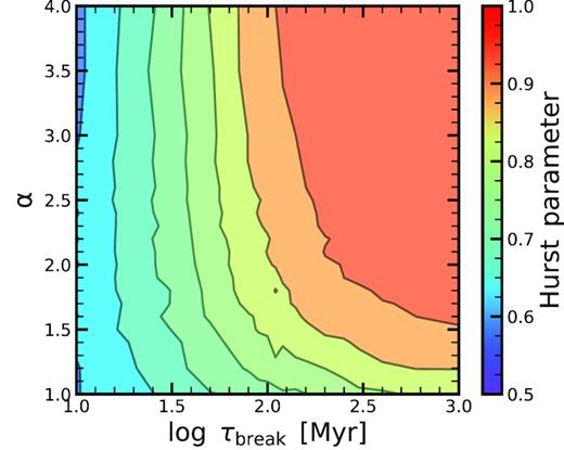
Hurst parameter, H, in the plane of the break time-scale τ_break and power-law slope α of the PSD. H increases towards ∼1 with increasing τ_break and α, consistent with the SFHs shown in Figs 1 and 2. At α > 2 and log τ_break/Myr > 1.5, the Hurst parameter converges to ∼1 and is not able to quantify any differences in the PSD.

Open in new tab Download slide

APPENDIX B: RECOVERING PARAMETERS OF THE POWER SPECTRUM DENSITY

B1 Non-stationarity of the mean star-formation rate

As discussed in the body of the text, our main assumption was that the star-forming galaxies move in stochastic fashion around the MS. We have also shown that our approach allows a lot of flexibility and covers even cases where individual galaxies do not significantly fluctuate around the MS within the cosmological time-scale. This is in general true for SFH histories created with large α and long τ_break (see Fig. 1).

Nevertheless, the question arises whether an additional long-term component in the SFH would bias our result and lead to errors when measuring α and τ_break. We have argued in Section 5.2.2 that any change of MS should be minimal during the time that influences the result of our analysis in Section 5. Here we extend this analysis, and conduct a test where we consider the change in effective α and τ_break after we have added a smooth, log-normal SFH to our simulated SFHs.

First, in order to estimate the intrinsic uncertainty to measure α and τ_break, we compute the PSD from the modelled SFHs (see Fig. 2) and then fit for α and τ_break in the frequency range log (f/Myr⁻¹) = −3.0 to log (f/Myr⁻¹) = −0.5. The best-fitting α and τ_break are shown in with the blue contours and blue points with errorbars in Fig. B1. The contours (and errorbars) mark the scatter (16th–84th percentiles) obtained fitting α and τ_break for 1000 SFHs. We see that, as expected, we are always able to recover α and τ_break within the narrow uncertainty range. In general, we find that the input parameters can be better recovered for ‘bursty’ SFHs that vary on short time-scales than from ‘smooth’ SFHs that vary on longer time-scales.

Figure B1.

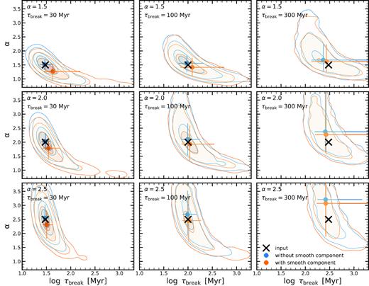
Recovery of the PSD parameters α and τ_break. Each panel shows the recovery test for a different α and τ_break. The input α and τ_break and marked by the black cross. The best-fitting PSD parameters are then indicated with the contours and points with errorbars. The blue shows the best-fit for the simulated SFHs, i.e. indicates the overall uncertainty in recovering the parameters of the power spectrum, while the orange shows the best-fit for the case where we have added an additional component to the SFH.

Open in new tab Download slide

We now repeat this test, but add an additional component to all of the simulated SFHs. We assume an additional log-normal star-formation component following the parametrization of Gladders et al. (2013) with (ln (T₀/Gyr), τ/Gyr) = (1.0, 1.5), which leads to the SFH that declines by about 0.8 dex over the past ∼4 Gyr. Following the same fitting procedure as described above, we show the best-fitting results in Fig. B1 with the orange contours and points with errorbars. The input PSD parameters are within the errorbars of the estimated PSD parameters. For the SFHs with a high burstiness (small α and short τ_break), we find that the recovered α is biased low compared to the input value, while the recovered τ_break tends to be biased high compared to the input value. The opposite is true for SFHs generated with large α and long τ_break.

Overall, we have shown here that the measurements of parameters describing the PSD (α and |$\tau$|⁠) are robust against the addition of a singular long-term SFH component to the whole galaxy population. This can be explained by the fact that this long-term component only contributes to the smallest frequency (longest time-scale) in the PSD.

B2 Effect of changing the intrinsic σ_MS assumption

Here we shortly discuss the effects of the different assumptions for the value for the underlying intrinsic σ_MS. As we have indicated in Section 2.2, we have used σ_MS = 0.4 throughout this work. This has been motivated by the measured |$\sigma _{\rm H_{\rm \alpha }}$| value and the fact that very quickly reacting H α follows closely real star-formation so the |$\sigma _{\rm H_{\rm \alpha }}$| is largely representative of the intrinsic σ_MS. Additionally, we have used the ratios of measured widths of the MS to infer the area of allowed α and τ_break parameter space, as this minimizes the influence of the underlying intrinsic σ_MS on the final result (see Appendix C).

In Fig. B2 we show recreation of Fig. 12, with very different values for intrinsic σ_MS (0.2 and 0.6), to show qualitatively the changes of the deduced parameters. We emphasize again that these assumed values are outside of what we would expect given the Davis et al. (2019) data. We still see roughly the same degeneracy in the shape of the allowed parameter space. For the cases shown in figure and when assuming α = 2, we find |$\tau _{\rm break}=74^{+46}_{-31}$| Myr for the case of σ_MS = 0.2 and |$\tau _{\rm break}=295^{+295}_{-147}$| Myr for the case with σ_MS = 0.6. We note that even in this case with large deviations from the fiducial value for σ_MS, we find the τ_break that are needed to explain the data are on the order of ∼100 Myr.

Figure B2.

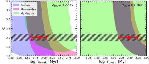
Effect of large changes to assumed intrinsic σ_MS. We show the observational constraints derived from ratios of measured widths of the Main Sequence in different indicators from Fig. 12, but assume σ_MS = 0.2 dex (left-hand panel) and σ_MS = 0.6 dex (right-hand panel).

Open in new tab Download slide

APPENDIX C: CONNECTION BETWEEN STAR-FORMATION MEASUREMENTS IN DIFFERENT INDICATORS

In this appendix we extend our analytical calculation of the measured width of MS, as seen after measurement in different indicators. We start by noticing that the star formation rate measured by a given indicator is connected to the previous star formation and is given by the intensity of that star-formation episode and a response of that particular indicator to the star formation, i.e.

\begin{eqnarray*} \mathrm{SFR}_{\rm ind}(t)=\mathrm{SFR}(t^{\prime }) f_{\rm ind}(t-t^{\prime }), \end{eqnarray*}

(C1)

where SFR_ind is the measured star-formation, SFR is the actual star-formation, and f_ind are response functions (the ones that we have used in this work are presented in Appendix D). In the case of continuous star-formation the measured star-formation is given by

\begin{eqnarray*} \mathrm{SFR}_{\rm ind}(t)=\int ^{t}_{-\infty } \mathrm{SFR}(t^{\prime }) f_{\rm ind}(t-t^{\prime }) \mathrm{ \mathrm{ d}}t^{\prime }, \end{eqnarray*}

(C2)

where we have convolved the total SFH with an appropriate response function up to the time of the measurement. When discretized the above integral is written as a sum

\begin{eqnarray*} \mathrm{SFR}_{\rm ind}(t_{i})= \sum ^{\infty }_{t_{j}=0} \mathrm{SFR}(t_{i}-t_{j}) w_{\rm ind}(t_{j}), \end{eqnarray*}

(C3)

where SFR_ind(t_i) is the measured star-formation in bin t_i and w_ind(t_j) is the discretized version of the response function:

\begin{eqnarray*} w_{\rm ind}(t_{j}) = \int ^{t_{j}+\delta /2}_{t_{j}-\delta /2} f_{\rm ind}(t^{\prime }) \mathrm{ d}t^{\prime }, \end{eqnarray*}

(C4)

where δ is the duration of the discretization bin. In this work we use δ = 1 Myr (see Section 2 for justification of this time-scale).

Now, consider the ensemble of galaxies moving around Main-Sequence in stochastic fashion with a log-normal distribution function. Let us denote with Δ⁵ log -distance from the median value of MS i.e. (see equations 8 and 9):

\begin{eqnarray*} \Delta =\log \mathrm{SFR} - \log \mathrm{SFR}_{\rm MS}. \end{eqnarray*}

(C5)

We rewrite the equation (C3) in terms of Δ:

\begin{eqnarray*} \Delta _{\rm ind}(t_i)= \log \sum ^{\infty }_{t_j=0} 10^{\Delta (t_i-t_j)} w_{\rm ind}(t_j). \end{eqnarray*}

(C6)

We note that factors in the exponent Δ(i − j) are in general expected to be small as they are bound by the width of the MS. In that case we can use the MacLauren expansion:

\begin{eqnarray*} 10^{x}= 1+\ln (10)x+\frac{1}{2}\ln (10)^{2}x^{2}+\frac{1}{6}\ln (10)^{3}x^{3}+... \end{eqnarray*}

(C7)

Let us continue by taking first two orders of expansion above in equation (C7):

\begin{eqnarray*} \Delta _{\rm ind}(t_{i}) &=& \log \sum ^{\infty }_{j=0} \left(1 + \ln (10)\Delta (t_{i}-t_{j}) \right. \nonumber\\ && \left.+ \,\frac{1}{2}\ln (10)^{2}\Delta ^{2}(t_{i}-t_{j})+....\right) w_{\rm ind} (t_{j})\nonumber\\ &=& \log \left[ \left(\sum ^{\infty }_{j=0}w_{\rm ind}(t_{j})\right)+\ln (10)\left(\sum ^{\infty }_{t_{j}=0} \Delta (t_{i}-t_{j}) w_{\rm ind}(t_{j})\!\!\right) \right. \nonumber\\ &&\left.+\, \frac{1}{2}\ln (10)^{2} \left(\sum ^{\infty }_{t_{j}=0} \Delta ^{2}(t_{i}-t_{j})w_{\rm ind}(t_{j})\right)+....\right] \nonumber\\ &=& \log \left[1+ \ln (10) \sum ^{\infty }_{t_{j}=0} \Delta (t_{i}-t_{j}) w_{\rm ind}(t_{j}) \right. \nonumber\\ &&\left. +\, \frac{1}{2}\ln (10)^{2} \left(\sum ^{\infty }_{t_{j}=0} \Delta ^{2}(t_{i}-t_{j})w_{\rm ind}(t_{j})\right)+....\right], \end{eqnarray*}

(C8)

where we have used the property that the response function has to sum to unity, i.e. |$\sum ^{\infty }_{t_{j}=0}w_{\rm ind}(t_{j})=1$|⁠. We now expand the log function using

\begin{eqnarray*} \log (1+ x)=\frac{x}{\ln (10)}-\frac{x^{2}}{2 \ln (10)}+\frac{x^{3}}{3\ln (10)} +... \end{eqnarray*}

(C9)

and we find the expression

\begin{eqnarray*} \Delta _{\rm ind}(t_{i}) &=& \sum ^{\infty }_{t_{j}=0} \Delta (t_{i}-t_{j}) w_{\rm ind}(t_{j}) \nonumber\\ &&+\, \frac{\ln (10)}{2} \left[ \left(\sum ^{\infty }_{t_{j}=0} \Delta ^{2}(t_{i}-t_{j})w_{\rm ind}(t_{j})\right)\right.\nonumber\\ && \left.-\left(\sum ^{\infty }_{t_{j}=0} \Delta (t_{i}-t_{j}) w_{\rm ind}(t_{j}) \right)^{2} \right] +\ldots \end{eqnarray*}

(C10)

Let us now find variance of the measured MS after considering only the first term of the expansion above:

\begin{eqnarray*} \sigma ^{2}_{\rm ind,MS} (t_i)&=&\mbox{VAR} \left(\sum ^{\infty }_{t_{j}=0}\Delta (t_{i}-t_{j})w_{\rm ind}(t_j)\right) \nonumber\\ &=& \sum ^{\infty }_{t_{j}=0} \sum ^{\infty }_{t_{j^{^{\prime }}}=0} E(\Delta (t_{i}-t_{j})w_{\rm ind}(t_{j}) \Delta (t_{i}-t_{j^{^{\prime }}})w_{\rm ind}(t_{j^{^{\prime }}}))\nonumber\\ &&-\, E(\Delta (t_{i}-t_{j})w_{\rm ind}(t_{j})) E(\Delta (t_{i}-t_{j^{^{\prime }}})w_{\rm ind}(t_{j^{^{\prime }}}) ) \nonumber\\ &=& \sum ^{\infty }_{t_{j}=0} \sum ^{\infty }_{t_{j^{^{\prime }}}=0} w_{\rm ind}(t_{j}) w_{\rm ind}(t_{j^{^{\prime }}}) E(\Delta (t_{i}-t_{j}) \Delta (t_{i}-t_{j^{^{\prime }}})) \nonumber\\ &=& \sum ^{\infty }_{t_{j}=0} \sum ^{\infty }_{t_{j^{^{\prime }}}=0} w_{\rm ind} (t_{j}) w_{\rm ind}(t_{j^{^{\prime }}}) \cdot COV (\Delta (t_{i}-t_{j}), \nonumber\\ &&\Delta (t_{i}-t_{j^{^{\prime }}})) \nonumber\\ &=& \sigma ^{2}_{\rm MS} \sum ^{\infty }_{t_{j}=0}\sum ^{\infty }_{t_{j^{^{\prime }}}=0} w_{\rm ind}(t_{j}) w_{\rm ind}(t_{j^{^{\prime }}}) ACF(t_{j}-t_{j^{^{\prime }}}), \end{eqnarray*}

(C11)

where we have used the fact that the co-variance of the process is given by COV(Δ(t_i), Δ(t_j) = |$\sigma ^{2}_{\rm MS} ACF(t_{i}-t_{j})$| and where we have used symbol E to denote expectation value. We have also used the definition of the covariance together with the fact that the expectation value of a stationary process equals zero:

\begin{eqnarray*} COV\left(\Delta (t_{i}-t_{j}) \Delta (t_{i})\right) &=& E\left(\Delta (t_{i}-t_{j}) \Delta (t_{i})\right) \nonumber\\ &&-\,E\left(\Delta (t_{i}-t_{j})\right) E\left(\Delta (t_{i})\right) \nonumber\\ &=& E\left(\Delta (t_{i}-t_{j}) \Delta (t_{i})\right). \end{eqnarray*}

(C12)

Taking into the account next order terms in equation (C10) will lead to extra terms in the summation (C11), with the smallest order being proportional to |$\sigma ^{4}_{\rm MS}$|⁠. This is because all |$\sigma ^{3}_{\rm MS}$| terms will inevitably be connected with terms E(Δ²(t_i)) · E(Δ(t_j)) or E(Δ(t_i)) · E(Δ²(t_j)) which are equal to zero, given the stationary of our problem. For the realistic widths of MS (σ_MS ∼ 0.4 ± 0.1) these |$\sigma ^{4}_{\rm MS}$| terms are sub-dominant and therefore lead only to relatively small corrections (e.g. see the relatively small difference between the input and recovered parameters in Figs 6 and 7).

In the simplest case, discussed in Section 3, in which we assume that a given SFR indicator is given by a step function lasting N_j time units, i.e.

\begin{eqnarray*} w_{\rm ind}(t_{j}) = \left\lbrace \begin{array}{@{}l@{\quad }l@{}}1/N_{j} & 1 \le t_j \le N_{j} \\ 0 &\text{otherwise.} \end{array}\right. \end{eqnarray*}

the last expression in equation (C11) can be written as

\begin{eqnarray*} \sigma ^{2}_{\rm ind,MS} (t_{i})=\frac{\sigma ^{2}_{\rm MS}}{N^{2}_{j}} \sum _{t_{j}=1}^{N_{j}}\sum _{t_{j^{^{\prime }}}=1}^{N_{j}} ACF (t_{j}-t_{j^{^{\prime }}}), \end{eqnarray*}

(C13)

and we can now recognize equation (15) used in the main body of the text.

APPENDIX D: LUMINOSITY EVOLUTION OF A SIMPLE STELLAR POPULATION (SSP)

As we have extensively discussed in the main text of the paper, the ability to differentiate different stochastic processes that govern star-formation is dependent on being able to measure the SFR with different indicators that probe different time-scales. To be sensitive to a wider range of different PSDs, these response functions of the SFR indicators would ideally be well differentiated and cover a large range of time-scales. We show in Fig. D1 the luminosity evolution, seen in different passbands, of a Simple Stellar Population (SSP). These are effective response functions, i.e. the observed SFH in any of these bands can be considered as a convolution of the intrinsic SFH with these luminosity evolutions. In the left-hand panel, we see that all of the traces exhibit peak at early times (∼5 Myr), followed by an exponential-like decline. The right-hand panel shows the cumulative luminosity evolution, indicating more clearly the long-term behaviour of the different indicators. H α responds very quickly to star-formation – therefore, the measurement of the MS width in H α is very similar to the intrinsic MS width for almost the whole range of parameter space that we have considered, as seen in Fig. 10. As expected, the indicators corresponding to longer wavelengths tend to have slower responses, showing long ‘memory’ of the previous SFH. The fact that all of these indicators are a mixture of the recent and long-term star-formation complicates matters and makes the interpretation of the measurements, such as width of MS, quite unintuitive, but they can be modelled through simulations (Fig. 10).

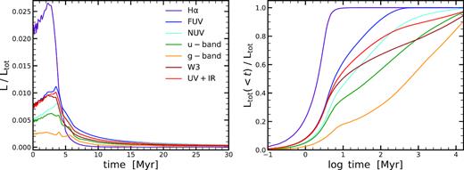
$Luminosity evolution of different SFR tracers for a Simple Stellar Population (SSP). The left-hand panel shows the luminosity as a function of time (L(t)), in bins of 0.1 Myr, normalized by total luminosity emitted over 25 Gyr ($L_{\rm tot},~ L_{\rm tot}\equiv \int ^{25\mathrm{Gyr}}_{0}L(t)\mathrm{ d}t$). The right-hand panel shows the cumulative luminosity evolution. The purple, blue, cyan, green, orange, and red line show the luminosity of the H α emission line, FUV band, NUV band, u band, g band, WISE-3 band, and UV+IR, respectively. Clearly, the H α emission line has the fastest reaction time-scale ($50{{\ \rm per\ cent}}$ of the total luminosity is emitted in the first ∼3 Myr), followed by the FUV and other traces which test redder part of the spectrum.$

Figure D1.

Luminosity evolution of different SFR tracers for a Simple Stellar Population (SSP). The left-hand panel shows the luminosity as a function of time (L(t)), in bins of 0.1 Myr, normalized by total luminosity emitted over 25 Gyr (⁠|$L_{\rm tot},~ L_{\rm tot}\equiv \int ^{25\mathrm{Gyr}}_{0}L(t)\mathrm{ d}t$|⁠). The right-hand panel shows the cumulative luminosity evolution. The purple, blue, cyan, green, orange, and red line show the luminosity of the H α emission line, FUV band, NUV band, u band, g band, WISE-3 band, and UV+IR, respectively. Clearly, the H α emission line has the fastest reaction time-scale (⁠|$50{{\ \rm per\ cent}}$| of the total luminosity is emitted in the first ∼3 Myr), followed by the FUV and other traces which test redder part of the spectrum.

Open in new tab Download slide

APPENDIX E: TIME-SCALES OF DIFFERENT SFR TRACERS

We have shown in the main body of the manuscript how the key relations are simplified and well understood in the case where the SFR response function is a simple step function. On the other hand, in Appendix D we show that the real response functions have non-trivial time dependence and that they are clearly not well described by a step function. Crucially, the time-scales that best approximate different SFR tracers actually depend on the property of the SFH itself. In practice, similar to the derivation of the luminosity-SFR calibration, one usually assumes a constant SFR and then determines the luminosity-weighted mean age of the stellar population (e.g. Kennicutt 1998; Kennicutt & Evans 2012; Madau & Dickinson 2014). A more sophisticated approach is to consider more realistic SFHs from numerical and analytical simulations, with the caveat that the variability of the SFHs is simulation-dependent and it might bias the measurement (e.g. Tacchella et al. 2018). Already Johnson et al. (2013) showed – based on empirical SFHs – that fluctuations in the SFHs alone can cause factor of ∼2 variations in the UV luminosities relative to the assumption of a constant SFH over the past 100 Myr. Thanks to our framework of stochastic SFHs introduced in Section 2, we are able to generate and understand SFHs that have different variability properties according to a power spectral density.

Here we are looking to derive a singular time-scale over which to average the realistic star-formation response to best approximate complex and realistic functions with a step function of a given duration. We will first briefly express our problem analytically and afterwards derive these time-scales numerically for the different indicators that we used in Section 4 (H α, FUV, NUV, u, W3, and UV+IR).

The statement about approximating realistic star-formation responses as a step function can be expressed as a search for the best N_approx to approximate equation (C6):

\begin{eqnarray*} \lt \Delta (t_{i})\gt _{N_{\rm approx}}\cong \log \sum ^{\infty }_{t_{j}=1} 10^{\Delta (t_{i}-t_{j})} w_{\rm ind}(t_{j}), \end{eqnarray*}

(E1)

where

\begin{eqnarray*} {\lt} \Delta (t_{i})\gt _{N_{\rm approx}}=\log \sum ^{N_{\rm approx}}_{t_{j}=1} 10^{\Delta (t_{i}-t_{j})} . \end{eqnarray*}

(E2)

Comparing the expressions within the logarithms we see that the condition simplifies to the following equation for N_approx:

\begin{eqnarray*} \sum ^{N_{\rm approx}}_{t_{j}=1} 10^{\Delta (t_{i}-t_{j})} =\sum ^{\infty }_{t_{j}=0} 10^{\Delta (t_{i}-t_{j})} w_{\rm ind}(t_{j}). \end{eqnarray*}

(E3)

From here we can see that in order to derive N_approx we have to consider both the properties of stochastic process, that govern time dependence of Δ(t_i − t_j) term, and various indicators with their response function described with w_ind(t_j). In other words, as stated before, the time-scale associated with each SFR traces depend on the previous SFH (in addition to the properties of each indicator).

In order to derive the time-scales of the different SFR tracers numerically, we generate SFHs with different α and τ_break, as described in Section 2. We estimate the time-scale of the SFR tracer by solving equation (E1) in a statistical sense, by minimizing the RMS difference of the SFR of the tracer and the intrinsic SFR averaged over different time-scales. In other words, we search for N_approx that minimizes the variance of the quantity |$\Delta _{\rm ind}(t_{i})-\lt \Delta (t_{i})\gt _{N_{\rm approx}}$|⁠.

In Fig. E1, we present the result of this analysis for H α, FUV, NUV, u,W3, and UV+IR. As expected, H α corresponds to shortest time-scale while UV+IR and u-band correspond to longer time-scales (e.g. see Fig. D1). We however note large variations across the parameter space of τ and α, confirming our intuition about the importance of considering the underlying stochastic process on making a statement about time-scales probed by different indicators. The differences are obviously larger for the longer indicators. Intuitively, when the indicator is very quick, as is the case for H α or FUV, effect of ‘mixing in’ of the underlying process is reduced and changes of τ_break and α that affect longer time-scale are not probed in this analysis.

Figure E1.

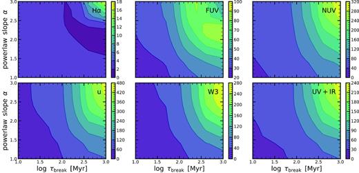
Effective time-scale for different SFR tracers, as a function of parameters describing the underlying stochastic process (α and τ_break). Effective time-scale is defined as a time-scale over which the averaged SFH is most similar to actual SFR measured in a given indicator, and is indicated by the colour bar for each panel. This time-scale depend not only on the indicator used, but also on the parameters of the stochastic process. To the first order, the burstier the SFH (see Section 2.4), the shorter the time-scale. Furthermore, the H α and FUV SFR indicators trace the shortest time-scale.

Open in new tab Download slide

For the set of parameters that we have deduced in Section 5, α = 2 and |$\tau _{\rm break}=170^{+169}_{-85}~\mathrm{Myr}$|⁠, we find that the effective times of the indicators are |$t_{\rm eff} (\mbox{H}\alpha)=2.0_{-0.1}^{+0.4}~\mathrm{Myr}$|⁠, |$t_{\rm eff} (\mbox{FUV})=63_{-1}^{+2}~\mathrm{Myr}$|⁠, |$t_{\rm eff} (\mbox{NUV})=119_{-2}^{+8}~\mathrm{Myr}$|⁠, |$t_{\rm eff} (\mbox{u-band})=164_{-16}^{+15}~\mathrm{Myr}$|⁠, |$t_{\rm eff} (\mbox{W3})=96_{-14}^{+7}~\mathrm{Myr}$|⁠, and |$t_{\rm eff} (\mbox{UV{+}IR})=84_{-5}^{+6}~\mathrm{Myr}$|⁠. Of course, these estimates suffer from the same caveats that we have discussed in Sections 5 and just therefore only be taken as a general guidance, rather than strict quantitative measurement.

This article is published and distributed under the terms of the Oxford University Press, Standard Journals Publication Model (https://dbpia.nl.go.kr/journals/pages/open_access/funder_policies/chorus/standard_publication_model)

Download all slides

Month:	Total Views:
May 2019	4
June 2019	18
July 2019	24
August 2019	16
September 2019	20
October 2019	23
November 2019	9
December 2019	10
January 2020	13
February 2020	15
March 2020	7
April 2020	8
May 2020	14
June 2020	24
July 2020	35
August 2020	19
September 2020	26
October 2020	22
November 2020	13
December 2020	12
January 2021	17
February 2021	32
March 2021	24
April 2021	14
May 2021	10
June 2021	28
July 2021	24
August 2021	18
September 2021	20
October 2021	34
November 2021	27
December 2021	24
January 2022	33
February 2022	22
March 2022	8
April 2022	10
May 2022	14
June 2022	17
July 2022	31
August 2022	34
September 2022	35
October 2022	45
November 2022	26
December 2022	17
January 2023	34
February 2023	21
March 2023	33
April 2023	26
May 2023	25
June 2023	13
July 2023	34
August 2023	27
September 2023	32
October 2023	45
November 2023	45
December 2023	37
January 2024	47
February 2024	36
March 2024	47
April 2024	50
May 2024	42
June 2024	55
July 2024	71
August 2024	48
September 2024	48
October 2024	45
November 2024	51
December 2024	23
January 2025	23
February 2025	14
March 2025	33
April 2025	39
May 2025	9

Article Contents

Stochastic modelling of star-formation histories I: the scatter of the star-forming main sequence

ABSTRACT

1 INTRODUCTION

2 DESCRIPTION OF STAR-FORMATION HISTORIES WITH STOCHASTIC PROCESSES

2.1 Assumptions

2.2 General description of stochastic processes

2.3 Generating star-formation histories

2.4 Quantifying the burstiness of star-formation histories

3 FINDING PARAMETERS OF STOCHASTIC STAR-FORMATION HISTORY IN A TOY MODEL

3.1 Impact of averaging of the star-formation histories on the shape of the measured MS

3.1.1 Mean measured offset from the main sequence

3.1.2 Width of the MS

3.2 Comparison to numerically generated model galaxies

3.3 Measuring parameters of stochastic process from the mock data

4 FINDING PARAMETERS OF STOCHASTIC STAR-FORMATION HISTORY WITH REALISTIC RESPONSE FUNCTIONS

4.1 SFR tracers

4.2 Shape of the MS as seen by different SFR indicators: normalization and scatter

4.3 Ratio of SFRs with different indicators

5 OBSERVATIONAL CONSTRAINTS

5.1 Main result

5.2 Discussion

5.2.1 Mass dependence

5.2.2 Caveats

6 SUMMARY AND CONCLUSIONS

ACKNOWLEDGEMENTS

Footnotes

REFERENCES

APPENDIX A: FRACTIONAL BROWNIAN MOTION AND HURST PARAMETER

APPENDIX B: RECOVERING PARAMETERS OF THE POWER SPECTRUM DENSITY

B1 Non-stationarity of the mean star-formation rate

B2 Effect of changing the intrinsic σMS assumption

APPENDIX C: CONNECTION BETWEEN STAR-FORMATION MEASUREMENTS IN DIFFERENT INDICATORS

APPENDIX D: LUMINOSITY EVOLUTION OF A SIMPLE STELLAR POPULATION (SSP)

APPENDIX E: TIME-SCALES OF DIFFERENT SFR TRACERS

Citations

Views

Altmetric

Email alerts

Astrophysics Data System

Citing articles via

Latest

Most Read

Most Cited

This Feature Is Available To Subscribers Only

B2 Effect of changing the intrinsic σ_MS assumption