Modelling accretion disc emission with generalized temperature profile and its effect on AGN spectral energy distribution

Basic information of our sample AGN.

No.	Object	RA	Dec.	Redshift	\|$E(B-V)_{\rm G}^{\dagger }$\|	Swift ObsID	SDSS SpecObjlD
							(Plate-MJD-Fiber)
1	Mrk 1018	02 06 15.9	– 00 17 29	0.0424	0.028	00035166001	0404–51812–0141
2	MCG 04-22-042	09 23 43.0	+ 22 54 33	0.0323	0.043	00035263001	2290–53727–0578
3	Mrk 705	09 26 03.3	+ 12 44 04	0.0292	0.041	00090998001	2578–54093–0195
4	RX J1007.1 + 2203	10 07 10.2	+ 22 03 02	0.0820	0.032	00036537002	2364–53737–0458
5	CBS 126	10 13 03.2	+ 35 51 24	0.0791	0.011	00035306001	1951–53389–0614
6	Mrk 141	10 19 12.6	+ 63 58 03	0.0417	0.010	00035765001	0488–51914–0161
7	Mrk 142	10 25 31.3	+ 51 40 35	0.0449	0.016	00036539002	1008–52707–0558
8	Ton 1388	11 19 08.7	+ 21 19 18	0.1765	0.022	00035767001	6430–56299–0516
9	SBS 1136 + 594	11 39 08.9	+ 59 11 55	0.0601	0.014	00035265001	7099–56666–0869
10	PG 1138 + 222	11 41 16.1	+ 21 56 21	0.0632	0.027	00036541001	2504–54179–0639
11	KUG 1141 + 371	11 44 29.9	+ 36 53 09	0.0381	0.019	00091632001	1997–53442–0126
12	Mrk 1310	12 01 14.3	– 03 40 41	0.0196	0.031	00091002003	0331–52368–0121
13	RX J1209.8 + 3217	12 09 45.2	+ 32 17 02	0.1444	0.017	00035769006	2004–53737–0466
14	Mrk 50	12 23 24.1	+ 02 40 45	0.0234	0.016	00080077001	0519–52283–0487
15	Mrk 771	12 32 03.6	+ 20 09 29	0.0630	0.027	00080082001	2613–54481–0342
16	PG 1307 + 085	13 09 47.0	+ 08 19 48	0.1550	0.033	00037571001	1795–54507–0457
17	Ton 730	13 43 56.7	+ 25 38 48	0.0866	0.013	00037572002	2246–53767–0066
18	RX J1355.2 + 5612	13 55 16.6	+ 56 12 45	0.1219	0.007	00036547001	1323–52797–0443
19	Mrk 1392	15 05 56.5	+ 03 42 26	0.0361	0.047	00081174001	0589–52055–0111
20	Mrk 290	15 35 52.3	+ 57 54 09	0.0296	0.015	00080152003	0615–52347–0108
21	Mrk 493	15 59 09.6	+ 35 01 47	0.0313	0.024	00035080001	1417–53141–0078
22	KUG 1618 + 410	16 19 51.3	+ 40 58 48	0.0379	0.007	00036548001	1171–52753–0166
23	RX J1702.5 + 3247	17 02 31.1	+ 32 47 20	0.1633	0.023	00035771002	0973–52426–0114

No.	Object	RA	Dec.	Redshift	\|$E(B-V)_{\rm G}^{\dagger }$\|	Swift ObsID	SDSS SpecObjlD
							(Plate-MJD-Fiber)
1	Mrk 1018	02 06 15.9	– 00 17 29	0.0424	0.028	00035166001	0404–51812–0141
2	MCG 04-22-042	09 23 43.0	+ 22 54 33	0.0323	0.043	00035263001	2290–53727–0578
3	Mrk 705	09 26 03.3	+ 12 44 04	0.0292	0.041	00090998001	2578–54093–0195
4	RX J1007.1 + 2203	10 07 10.2	+ 22 03 02	0.0820	0.032	00036537002	2364–53737–0458
5	CBS 126	10 13 03.2	+ 35 51 24	0.0791	0.011	00035306001	1951–53389–0614
6	Mrk 141	10 19 12.6	+ 63 58 03	0.0417	0.010	00035765001	0488–51914–0161
7	Mrk 142	10 25 31.3	+ 51 40 35	0.0449	0.016	00036539002	1008–52707–0558
8	Ton 1388	11 19 08.7	+ 21 19 18	0.1765	0.022	00035767001	6430–56299–0516
9	SBS 1136 + 594	11 39 08.9	+ 59 11 55	0.0601	0.014	00035265001	7099–56666–0869
10	PG 1138 + 222	11 41 16.1	+ 21 56 21	0.0632	0.027	00036541001	2504–54179–0639
11	KUG 1141 + 371	11 44 29.9	+ 36 53 09	0.0381	0.019	00091632001	1997–53442–0126
12	Mrk 1310	12 01 14.3	– 03 40 41	0.0196	0.031	00091002003	0331–52368–0121
13	RX J1209.8 + 3217	12 09 45.2	+ 32 17 02	0.1444	0.017	00035769006	2004–53737–0466
14	Mrk 50	12 23 24.1	+ 02 40 45	0.0234	0.016	00080077001	0519–52283–0487
15	Mrk 771	12 32 03.6	+ 20 09 29	0.0630	0.027	00080082001	2613–54481–0342
16	PG 1307 + 085	13 09 47.0	+ 08 19 48	0.1550	0.033	00037571001	1795–54507–0457
17	Ton 730	13 43 56.7	+ 25 38 48	0.0866	0.013	00037572002	2246–53767–0066
18	RX J1355.2 + 5612	13 55 16.6	+ 56 12 45	0.1219	0.007	00036547001	1323–52797–0443
19	Mrk 1392	15 05 56.5	+ 03 42 26	0.0361	0.047	00081174001	0589–52055–0111
20	Mrk 290	15 35 52.3	+ 57 54 09	0.0296	0.015	00080152003	0615–52347–0108
21	Mrk 493	15 59 09.6	+ 35 01 47	0.0313	0.024	00035080001	1417–53141–0078
22	KUG 1618 + 410	16 19 51.3	+ 40 58 48	0.0379	0.007	00036548001	1171–52753–0166
23	RX J1702.5 + 3247	17 02 31.1	+ 32 47 20	0.1633	0.023	00035771002	0973–52426–0114

Notes: †. Galactic reddening from Schlegel, Finkbeiner & Davis (1998).

Table 1.

Basic information of our sample AGN.

No.	Object	RA	Dec.	Redshift	\|$E(B-V)_{\rm G}^{\dagger }$\|	Swift ObsID	SDSS SpecObjlD
							(Plate-MJD-Fiber)
1	Mrk 1018	02 06 15.9	– 00 17 29	0.0424	0.028	00035166001	0404–51812–0141
2	MCG 04-22-042	09 23 43.0	+ 22 54 33	0.0323	0.043	00035263001	2290–53727–0578
3	Mrk 705	09 26 03.3	+ 12 44 04	0.0292	0.041	00090998001	2578–54093–0195
4	RX J1007.1 + 2203	10 07 10.2	+ 22 03 02	0.0820	0.032	00036537002	2364–53737–0458
5	CBS 126	10 13 03.2	+ 35 51 24	0.0791	0.011	00035306001	1951–53389–0614
6	Mrk 141	10 19 12.6	+ 63 58 03	0.0417	0.010	00035765001	0488–51914–0161
7	Mrk 142	10 25 31.3	+ 51 40 35	0.0449	0.016	00036539002	1008–52707–0558
8	Ton 1388	11 19 08.7	+ 21 19 18	0.1765	0.022	00035767001	6430–56299–0516
9	SBS 1136 + 594	11 39 08.9	+ 59 11 55	0.0601	0.014	00035265001	7099–56666–0869
10	PG 1138 + 222	11 41 16.1	+ 21 56 21	0.0632	0.027	00036541001	2504–54179–0639
11	KUG 1141 + 371	11 44 29.9	+ 36 53 09	0.0381	0.019	00091632001	1997–53442–0126
12	Mrk 1310	12 01 14.3	– 03 40 41	0.0196	0.031	00091002003	0331–52368–0121
13	RX J1209.8 + 3217	12 09 45.2	+ 32 17 02	0.1444	0.017	00035769006	2004–53737–0466
14	Mrk 50	12 23 24.1	+ 02 40 45	0.0234	0.016	00080077001	0519–52283–0487
15	Mrk 771	12 32 03.6	+ 20 09 29	0.0630	0.027	00080082001	2613–54481–0342
16	PG 1307 + 085	13 09 47.0	+ 08 19 48	0.1550	0.033	00037571001	1795–54507–0457
17	Ton 730	13 43 56.7	+ 25 38 48	0.0866	0.013	00037572002	2246–53767–0066
18	RX J1355.2 + 5612	13 55 16.6	+ 56 12 45	0.1219	0.007	00036547001	1323–52797–0443
19	Mrk 1392	15 05 56.5	+ 03 42 26	0.0361	0.047	00081174001	0589–52055–0111
20	Mrk 290	15 35 52.3	+ 57 54 09	0.0296	0.015	00080152003	0615–52347–0108
21	Mrk 493	15 59 09.6	+ 35 01 47	0.0313	0.024	00035080001	1417–53141–0078
22	KUG 1618 + 410	16 19 51.3	+ 40 58 48	0.0379	0.007	00036548001	1171–52753–0166
23	RX J1702.5 + 3247	17 02 31.1	+ 32 47 20	0.1633	0.023	00035771002	0973–52426–0114

No.	Object	RA	Dec.	Redshift	\|$E(B-V)_{\rm G}^{\dagger }$\|	Swift ObsID	SDSS SpecObjlD
							(Plate-MJD-Fiber)
1	Mrk 1018	02 06 15.9	– 00 17 29	0.0424	0.028	00035166001	0404–51812–0141
2	MCG 04-22-042	09 23 43.0	+ 22 54 33	0.0323	0.043	00035263001	2290–53727–0578
3	Mrk 705	09 26 03.3	+ 12 44 04	0.0292	0.041	00090998001	2578–54093–0195
4	RX J1007.1 + 2203	10 07 10.2	+ 22 03 02	0.0820	0.032	00036537002	2364–53737–0458
5	CBS 126	10 13 03.2	+ 35 51 24	0.0791	0.011	00035306001	1951–53389–0614
6	Mrk 141	10 19 12.6	+ 63 58 03	0.0417	0.010	00035765001	0488–51914–0161
7	Mrk 142	10 25 31.3	+ 51 40 35	0.0449	0.016	00036539002	1008–52707–0558
8	Ton 1388	11 19 08.7	+ 21 19 18	0.1765	0.022	00035767001	6430–56299–0516
9	SBS 1136 + 594	11 39 08.9	+ 59 11 55	0.0601	0.014	00035265001	7099–56666–0869
10	PG 1138 + 222	11 41 16.1	+ 21 56 21	0.0632	0.027	00036541001	2504–54179–0639
11	KUG 1141 + 371	11 44 29.9	+ 36 53 09	0.0381	0.019	00091632001	1997–53442–0126
12	Mrk 1310	12 01 14.3	– 03 40 41	0.0196	0.031	00091002003	0331–52368–0121
13	RX J1209.8 + 3217	12 09 45.2	+ 32 17 02	0.1444	0.017	00035769006	2004–53737–0466
14	Mrk 50	12 23 24.1	+ 02 40 45	0.0234	0.016	00080077001	0519–52283–0487
15	Mrk 771	12 32 03.6	+ 20 09 29	0.0630	0.027	00080082001	2613–54481–0342
16	PG 1307 + 085	13 09 47.0	+ 08 19 48	0.1550	0.033	00037571001	1795–54507–0457
17	Ton 730	13 43 56.7	+ 25 38 48	0.0866	0.013	00037572002	2246–53767–0066
18	RX J1355.2 + 5612	13 55 16.6	+ 56 12 45	0.1219	0.007	00036547001	1323–52797–0443
19	Mrk 1392	15 05 56.5	+ 03 42 26	0.0361	0.047	00081174001	0589–52055–0111
20	Mrk 290	15 35 52.3	+ 57 54 09	0.0296	0.015	00080152003	0615–52347–0108
21	Mrk 493	15 59 09.6	+ 35 01 47	0.0313	0.024	00035080001	1417–53141–0078
22	KUG 1618 + 410	16 19 51.3	+ 40 58 48	0.0379	0.007	00036548001	1171–52753–0166
23	RX J1702.5 + 3247	17 02 31.1	+ 32 47 20	0.1633	0.023	00035771002	0973–52426–0114

Notes: †. Galactic reddening from Schlegel, Finkbeiner & Davis (1998).

3 DATA REDUCTION

The reduction procedures of the optical/UV photometric data, the X-ray data, and the optical SDSS spectroscopic data are described in this section. We download the pipeline-processed ‘Level 2’ UVOT and XRT fits files from ASI Science Data Center.² For sources with multiple observations, we utilize the data with the maximum exposure time. The SDSS optical spectra are downloaded from SDSS Science Archive Server.³

3.1 UVOT data

All the sources in our sample have six UVOT filter photometric measurements in the optical (v, b, and u) and UV (uvw1, uvm2, and uvw2) bands. We follow the UVOT reduction threads⁴ for data reduction. The ‘Level 2’ UVOT fits files for each of the filters are summed together by using the procedure uvotimsum, and source magnitudes are extracted by using uvotsource. We use a circle source region with a radius of 5 arcsec centring on the source, and a background region with a radius of 20 arcsec selected from a source-free region close-by. At the UV wavelengths, the starlight contribution within the aperture is negligible, and we simply consider the measurement as being dominated by the AGN radiation. For the v, b, and u magnitudes, contamination from the host galaxy starlight may not be negligible, and we thus perform 2D image decomposition on the obtained images to decompose the AGN from the host galaxy. Such a procedure was also adopted in a similar work by Vasudevan et al. (2009) for UVOT data.

We use the galfit software developed by Peng et al. (2002) to perform 2D image decomposition. For each of the image, a point spread function (PSF) is constructed from nearby stars in the field of view (USNO A2.0 catalogue, Monet 1998) with count rates comparable to that of the target AGN. The background is calculated by selecting a source-free region near the source and is always included. The AGN is modelled with the point-like source (as an instrumental PSF), with an initial magnitude and position from the results of uvotsource. A potential galaxy component is added in, as either an exponential or a Sérsic model, whichever results in a better fit. Such a model is fitted to the image data of the three optical filters, resulting in good fits in all but one object (PG 1138 + 222), which is judged by visually examining the residual images. Among these, eight objects can be well fitted with a point-like source model in all of the three filters (i.e. the host galaxy starlight contribution is negligible), while in the remaining 14 objects an additional galactic component (exponential) is needed to improve the fits for at least two filters. An example of the 2D imaging fitting results is shown in Fig. 1. For PG 1138 + 222, no good fit can be achieved due to the poor data quality of the UVOT images. Since no host galaxy is seen apparently in the images, we consider them to be dominated by AGN emission, and simply use the 5 arcsec aperture photometric measurements as the AGN magnitudes.

Figure 1.

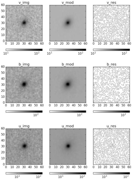
An example of 2D image decomposition results for Mrk 1310. The rows from top to bottom represent the results in v, b, and u bands, respectively. In each row, the first column shows the data image, the second column shows the best-fitting model (including the background component), and the third column shows the residual image derived by subtracting the model from the original data.

Finally, with the PSF magnitudes derived from galfit, we perform correction for coincidence-loss (the phenomenon when two or more photons arrive at a similar location on the detector within the same CCD readout interval, see Poole et al. 2008; Breeveld et al. 2010) in the optical filters.⁵ The best-estimated optical-to-UV magnitudes of the AGN for each of the filter bands are listed in Table 2, along with the magnitudes of the host galaxies in the optical filters for those with non-negligible host galaxy starlight. The magnitudes are corrected for the Galactic extinction by employing the idl code fm_unred.pro with E(B − V)_G given in Table 1, assuming the Milky Way (MW) extinction curve. No correction is made for the contamination to the continuum from AGN emission lines, which is considered to be negligible.⁶

Table 2.

UVOT photometry.

No.	Object	m_{v, AGN}	m_{v, ga}	m_{b, AGN}	m_{b, ga}	m_{u, AGN}	m_{u, ga}	m_{w1, AGN}	m_{m2, AGN}	m_{w2, AGN}
(1)	(2)	(3)	(4)	(5)	(6)	(7)	(8)	(9)	(10)	(11)
1	Mrk 1018	15.12	14.24	15.48	15.09	14.00	14.70	13.54	13.42	13.44
2	MCG 04-22-042	14.95	14.22	15.31	14.93	13.80	12.61	13.46	13.44	13.45
3	Mrk 705	15.11	14.25	15.59	15.34	14.28	15.04	14.04	13.95	14.02
4	RX J1007.1 + 2203	16.86	–	17.26	–	16.12	–	16.02	15.91	15.88
5	CBS 126	15.49	–	15.82	–	14.61	–	14.47	14.40	14.35
6	Mrk 141	15.94	14.97	16.42	15.79	15.47	15.74	15.29	15.34	15.40
7	Mrk 142	15.70	16.06	15.96	17.17	14.82	–	14.59	14.41	14.39
8	Ton 1388	14.43	–	14.55	–	13.23	–	13.00	12.82	12.92
9	SBS 1136 + 594	15.59	16.53	16.08	–	14.62	16.28	14.46	14.46	14.45
10	PG 1138 + 222	15.49	–	16.01	–	14.69	–	14.33	14.25	14.13
11	KUG 1141 + 371	16.90	15.53	17.24	16.34	16.08	16.80	15.84	15.99	16.04
12	Mrk 1310	16.74	15.07	17.41	15.83	15.54	15.22	15.52	15.59	15.64
13	RX J1209.8 + 3217	16.95	–	17.33	–	16.23	–	16.11	15.97	15.98
14	Mrk 50	16.00	15.21	16.25	15.85	14.76	15.66	14.56	14.60	14.63
15	Mrk 771	15.29	–	15.62	–	14.15	–	13.84	13.76	13.74
16	PG 1307 + 085	15.51	–	15.61	–	14.30	–	14.09	13.93	13.83
17	Ton 730	16.35	16.55	16.60	17.38	15.18	–	14.94	14.79	14.71
18	RX J1355.2 + 5612	16.37	–	16.93	–	15.86	–	15.76	15.64	15.72
19	Mrk 1392	15.21	14.25	15.60	15.02	14.31	15.15	13.87	13.77	13.81
20	Mrk 290	15.17	15.33	15.48	15.49	14.18	–	14.05	14.09	14.16
21	Mrk 493	15.38	14.16	15.63	14.81	15.42	14.66	14.19	14.15	14.22
22	KUG 1618 + 410	17.29	15.21	17.81	15.97	16.71	15.99	16.26	16.18	16.17
23	RX J1702.5 + 3247	15.45	–	15.71	–	14.54	–	14.46	14.36	14.47

No.	Object	m_{v, AGN}	m_{v, ga}	m_{b, AGN}	m_{b, ga}	m_{u, AGN}	m_{u, ga}	m_{w1, AGN}	m_{m2, AGN}	m_{w2, AGN}
(1)	(2)	(3)	(4)	(5)	(6)	(7)	(8)	(9)	(10)	(11)
1	Mrk 1018	15.12	14.24	15.48	15.09	14.00	14.70	13.54	13.42	13.44
2	MCG 04-22-042	14.95	14.22	15.31	14.93	13.80	12.61	13.46	13.44	13.45
3	Mrk 705	15.11	14.25	15.59	15.34	14.28	15.04	14.04	13.95	14.02
4	RX J1007.1 + 2203	16.86	–	17.26	–	16.12	–	16.02	15.91	15.88
5	CBS 126	15.49	–	15.82	–	14.61	–	14.47	14.40	14.35
6	Mrk 141	15.94	14.97	16.42	15.79	15.47	15.74	15.29	15.34	15.40
7	Mrk 142	15.70	16.06	15.96	17.17	14.82	–	14.59	14.41	14.39
8	Ton 1388	14.43	–	14.55	–	13.23	–	13.00	12.82	12.92
9	SBS 1136 + 594	15.59	16.53	16.08	–	14.62	16.28	14.46	14.46	14.45
10	PG 1138 + 222	15.49	–	16.01	–	14.69	–	14.33	14.25	14.13
11	KUG 1141 + 371	16.90	15.53	17.24	16.34	16.08	16.80	15.84	15.99	16.04
12	Mrk 1310	16.74	15.07	17.41	15.83	15.54	15.22	15.52	15.59	15.64
13	RX J1209.8 + 3217	16.95	–	17.33	–	16.23	–	16.11	15.97	15.98
14	Mrk 50	16.00	15.21	16.25	15.85	14.76	15.66	14.56	14.60	14.63
15	Mrk 771	15.29	–	15.62	–	14.15	–	13.84	13.76	13.74
16	PG 1307 + 085	15.51	–	15.61	–	14.30	–	14.09	13.93	13.83
17	Ton 730	16.35	16.55	16.60	17.38	15.18	–	14.94	14.79	14.71
18	RX J1355.2 + 5612	16.37	–	16.93	–	15.86	–	15.76	15.64	15.72
19	Mrk 1392	15.21	14.25	15.60	15.02	14.31	15.15	13.87	13.77	13.81
20	Mrk 290	15.17	15.33	15.48	15.49	14.18	–	14.05	14.09	14.16
21	Mrk 493	15.38	14.16	15.63	14.81	15.42	14.66	14.19	14.15	14.22
22	KUG 1618 + 410	17.29	15.21	17.81	15.97	16.71	15.99	16.26	16.18	16.17
23	RX J1702.5 + 3247	15.45	–	15.71	–	14.54	–	14.46	14.36	14.47

Notes: Column (1): identification number assigned in this paper. Column (2): NED name of the sample objects. Column (3): AGN magnitude in v band. Column (4): total magnitude of the host galaxy in v band. Column (5): AGN magnitude in b band. Column (6): total magnitude of the host galaxy in b band. Column (7): AGN magnitude in u band. Column (8): total magnitude of the host galaxy in u band. Column (9): AGN magnitude in uvw1 band. Column (10): AGN magnitude in uvm2 band. Column (11): AGN magnitude in uvw2 band. The magnitudes are the Vega magnitudes of Swift system (Poole et al. 2008). All the magnitudes have been corrected for the Galactic dust extinction.

Table 2.

UVOT photometry.

No.	Object	m_{v, AGN}	m_{v, ga}	m_{b, AGN}	m_{b, ga}	m_{u, AGN}	m_{u, ga}	m_{w1, AGN}	m_{m2, AGN}	m_{w2, AGN}
(1)	(2)	(3)	(4)	(5)	(6)	(7)	(8)	(9)	(10)	(11)
1	Mrk 1018	15.12	14.24	15.48	15.09	14.00	14.70	13.54	13.42	13.44
2	MCG 04-22-042	14.95	14.22	15.31	14.93	13.80	12.61	13.46	13.44	13.45
3	Mrk 705	15.11	14.25	15.59	15.34	14.28	15.04	14.04	13.95	14.02
4	RX J1007.1 + 2203	16.86	–	17.26	–	16.12	–	16.02	15.91	15.88
5	CBS 126	15.49	–	15.82	–	14.61	–	14.47	14.40	14.35
6	Mrk 141	15.94	14.97	16.42	15.79	15.47	15.74	15.29	15.34	15.40
7	Mrk 142	15.70	16.06	15.96	17.17	14.82	–	14.59	14.41	14.39
8	Ton 1388	14.43	–	14.55	–	13.23	–	13.00	12.82	12.92
9	SBS 1136 + 594	15.59	16.53	16.08	–	14.62	16.28	14.46	14.46	14.45
10	PG 1138 + 222	15.49	–	16.01	–	14.69	–	14.33	14.25	14.13
11	KUG 1141 + 371	16.90	15.53	17.24	16.34	16.08	16.80	15.84	15.99	16.04
12	Mrk 1310	16.74	15.07	17.41	15.83	15.54	15.22	15.52	15.59	15.64
13	RX J1209.8 + 3217	16.95	–	17.33	–	16.23	–	16.11	15.97	15.98
14	Mrk 50	16.00	15.21	16.25	15.85	14.76	15.66	14.56	14.60	14.63
15	Mrk 771	15.29	–	15.62	–	14.15	–	13.84	13.76	13.74
16	PG 1307 + 085	15.51	–	15.61	–	14.30	–	14.09	13.93	13.83
17	Ton 730	16.35	16.55	16.60	17.38	15.18	–	14.94	14.79	14.71
18	RX J1355.2 + 5612	16.37	–	16.93	–	15.86	–	15.76	15.64	15.72
19	Mrk 1392	15.21	14.25	15.60	15.02	14.31	15.15	13.87	13.77	13.81
20	Mrk 290	15.17	15.33	15.48	15.49	14.18	–	14.05	14.09	14.16
21	Mrk 493	15.38	14.16	15.63	14.81	15.42	14.66	14.19	14.15	14.22
22	KUG 1618 + 410	17.29	15.21	17.81	15.97	16.71	15.99	16.26	16.18	16.17
23	RX J1702.5 + 3247	15.45	–	15.71	–	14.54	–	14.46	14.36	14.47

No.	Object	m_{v, AGN}	m_{v, ga}	m_{b, AGN}	m_{b, ga}	m_{u, AGN}	m_{u, ga}	m_{w1, AGN}	m_{m2, AGN}	m_{w2, AGN}
(1)	(2)	(3)	(4)	(5)	(6)	(7)	(8)	(9)	(10)	(11)
1	Mrk 1018	15.12	14.24	15.48	15.09	14.00	14.70	13.54	13.42	13.44
2	MCG 04-22-042	14.95	14.22	15.31	14.93	13.80	12.61	13.46	13.44	13.45
3	Mrk 705	15.11	14.25	15.59	15.34	14.28	15.04	14.04	13.95	14.02
4	RX J1007.1 + 2203	16.86	–	17.26	–	16.12	–	16.02	15.91	15.88
5	CBS 126	15.49	–	15.82	–	14.61	–	14.47	14.40	14.35
6	Mrk 141	15.94	14.97	16.42	15.79	15.47	15.74	15.29	15.34	15.40
7	Mrk 142	15.70	16.06	15.96	17.17	14.82	–	14.59	14.41	14.39
8	Ton 1388	14.43	–	14.55	–	13.23	–	13.00	12.82	12.92
9	SBS 1136 + 594	15.59	16.53	16.08	–	14.62	16.28	14.46	14.46	14.45
10	PG 1138 + 222	15.49	–	16.01	–	14.69	–	14.33	14.25	14.13
11	KUG 1141 + 371	16.90	15.53	17.24	16.34	16.08	16.80	15.84	15.99	16.04
12	Mrk 1310	16.74	15.07	17.41	15.83	15.54	15.22	15.52	15.59	15.64
13	RX J1209.8 + 3217	16.95	–	17.33	–	16.23	–	16.11	15.97	15.98
14	Mrk 50	16.00	15.21	16.25	15.85	14.76	15.66	14.56	14.60	14.63
15	Mrk 771	15.29	–	15.62	–	14.15	–	13.84	13.76	13.74
16	PG 1307 + 085	15.51	–	15.61	–	14.30	–	14.09	13.93	13.83
17	Ton 730	16.35	16.55	16.60	17.38	15.18	–	14.94	14.79	14.71
18	RX J1355.2 + 5612	16.37	–	16.93	–	15.86	–	15.76	15.64	15.72
19	Mrk 1392	15.21	14.25	15.60	15.02	14.31	15.15	13.87	13.77	13.81
20	Mrk 290	15.17	15.33	15.48	15.49	14.18	–	14.05	14.09	14.16
21	Mrk 493	15.38	14.16	15.63	14.81	15.42	14.66	14.19	14.15	14.22
22	KUG 1618 + 410	17.29	15.21	17.81	15.97	16.71	15.99	16.26	16.18	16.17
23	RX J1702.5 + 3247	15.45	–	15.71	–	14.54	–	14.46	14.36	14.47

Notes: Column (1): identification number assigned in this paper. Column (2): NED name of the sample objects. Column (3): AGN magnitude in v band. Column (4): total magnitude of the host galaxy in v band. Column (5): AGN magnitude in b band. Column (6): total magnitude of the host galaxy in b band. Column (7): AGN magnitude in u band. Column (8): total magnitude of the host galaxy in u band. Column (9): AGN magnitude in uvw1 band. Column (10): AGN magnitude in uvm2 band. Column (11): AGN magnitude in uvw2 band. The magnitudes are the Vega magnitudes of Swift system (Poole et al. 2008). All the magnitudes have been corrected for the Galactic dust extinction.

3.2 XRT data

Of 23 XRT observations of the sample objects, 22 were performed in the photon counting (PC) mode and one in the windowed timing (WT) mode (Mrk 705). We follow the XRT analysis threads⁷ starting with ‘Level 2’ clean event fits files and employ xselect procedure to extract the source spectra. For the PC mode observation, the source photons are selected by using a circular region centred on the target with a typical radius of 47 arcsec, and the background photons from a close-by source-free region with r = 188 arcsec. For the WT mode, we use two circular regions with r = 47 arcsec for the source and background selection, respectively. We perform pile-up correction for sources with count rates larger than 0.5 counts s⁻¹ observed in PC mode by excluding a small region in the centre with a radius determined from ximage procedure. For Mrk 705, the observed count rate (∼0.6 counts s⁻¹) is much less than the threshold of pile-up (100 counts s⁻¹) for WT mode. X-ray events with grades from 0–12 are extracted to produce the X-ray spectra for the full energy range of the XRT (about 0.2–10 keV). For the extracted X-ray spectra, we use xrtmkarf to build the ancillary response files. The response matrix functions (RMFs) are determined individually by using quzcif. The source spectra are rebinned to have a minimum of 25 photons in each energy bin by using grppha (version 3.0.1). The information on the XRT data reduction is given in Table 3.

Table 3.

Log of XRT data reduction.

No.	Object	Mode	Exposure time	Source count rate	Background count rate
(1)	(2)	(3)	(4)	(5)	(6)
1	Mrk 1018	PC	5208	3.20	1.46
2	MCG 04-22-042	PC	9129	2.96	1.22
3	Mrk 705	WT	1773	5.94	10.3
4	RX J1007.1 + 2203	PC	11641	0.43	1.07
5	CBS 126	PC	4734	1.64	1.61
6	Mrk 141	PC	8156	1.18	1.56
7	Mrk 142	PC	2861	2.23	1.05
8	Ton 1388	PC	5090	2.71	1.38
9	SBS 1136 + 594	PC	9202	3.91	1.49
10	PG 1138 + 222	PC	4092	3.75	1.44
11	KUG 1141 + 371	PC	2680	1.39	1.08
12	Mrk 1310	PC	4054	1.43	2.02
13	RX J1209.8 + 3217	PC	17210	0.21	1.12
14	Mrk 50	PC	6399	3.95	1.61
15	Mrk 771	PC	6687	2.63	1.81
16	PG 1307 + 085	PC	8769	1.78	2.12
17	Ton 730	PC	11910	1.39	1.28
18	RX J1355.2 + 5612	PC	4398	1.01	1.55
19	Mrk 1392	PC	6331	2.60	1.93
20	Mrk 290	PC	5423	2.47	1.88
21	Mrk 493	PC	6978	2.15	1.30
22	KUG 1618 + 410	PC	2332	0.44	1.42
23	RX J1702.5 + 3247	PC	9144	2.00	1.33

No.	Object	Mode	Exposure time	Source count rate	Background count rate
(1)	(2)	(3)	(4)	(5)	(6)
1	Mrk 1018	PC	5208	3.20	1.46
2	MCG 04-22-042	PC	9129	2.96	1.22
3	Mrk 705	WT	1773	5.94	10.3
4	RX J1007.1 + 2203	PC	11641	0.43	1.07
5	CBS 126	PC	4734	1.64	1.61
6	Mrk 141	PC	8156	1.18	1.56
7	Mrk 142	PC	2861	2.23	1.05
8	Ton 1388	PC	5090	2.71	1.38
9	SBS 1136 + 594	PC	9202	3.91	1.49
10	PG 1138 + 222	PC	4092	3.75	1.44
11	KUG 1141 + 371	PC	2680	1.39	1.08
12	Mrk 1310	PC	4054	1.43	2.02
13	RX J1209.8 + 3217	PC	17210	0.21	1.12
14	Mrk 50	PC	6399	3.95	1.61
15	Mrk 771	PC	6687	2.63	1.81
16	PG 1307 + 085	PC	8769	1.78	2.12
17	Ton 730	PC	11910	1.39	1.28
18	RX J1355.2 + 5612	PC	4398	1.01	1.55
19	Mrk 1392	PC	6331	2.60	1.93
20	Mrk 290	PC	5423	2.47	1.88
21	Mrk 493	PC	6978	2.15	1.30
22	KUG 1618 + 410	PC	2332	0.44	1.42
23	RX J1702.5 + 3247	PC	9144	2.00	1.33

Notes: Column (1): identification number assigned in this paper. Column (2): NED name of the sample objects. Column (3): observational mode of XRT. Column (4): exposure time of XRT observation in unit of s⁻¹. Column (5): count rate of the source in unit of 10⁻¹ counts s⁻¹. Column (6): count rate of the background in unit of 10⁻² counts s⁻¹.

Table 3.

Log of XRT data reduction.

No.	Object	Mode	Exposure time	Source count rate	Background count rate
(1)	(2)	(3)	(4)	(5)	(6)
1	Mrk 1018	PC	5208	3.20	1.46
2	MCG 04-22-042	PC	9129	2.96	1.22
3	Mrk 705	WT	1773	5.94	10.3
4	RX J1007.1 + 2203	PC	11641	0.43	1.07
5	CBS 126	PC	4734	1.64	1.61
6	Mrk 141	PC	8156	1.18	1.56
7	Mrk 142	PC	2861	2.23	1.05
8	Ton 1388	PC	5090	2.71	1.38
9	SBS 1136 + 594	PC	9202	3.91	1.49
10	PG 1138 + 222	PC	4092	3.75	1.44
11	KUG 1141 + 371	PC	2680	1.39	1.08
12	Mrk 1310	PC	4054	1.43	2.02
13	RX J1209.8 + 3217	PC	17210	0.21	1.12
14	Mrk 50	PC	6399	3.95	1.61
15	Mrk 771	PC	6687	2.63	1.81
16	PG 1307 + 085	PC	8769	1.78	2.12
17	Ton 730	PC	11910	1.39	1.28
18	RX J1355.2 + 5612	PC	4398	1.01	1.55
19	Mrk 1392	PC	6331	2.60	1.93
20	Mrk 290	PC	5423	2.47	1.88
21	Mrk 493	PC	6978	2.15	1.30
22	KUG 1618 + 410	PC	2332	0.44	1.42
23	RX J1702.5 + 3247	PC	9144	2.00	1.33

No.	Object	Mode	Exposure time	Source count rate	Background count rate
(1)	(2)	(3)	(4)	(5)	(6)
1	Mrk 1018	PC	5208	3.20	1.46
2	MCG 04-22-042	PC	9129	2.96	1.22
3	Mrk 705	WT	1773	5.94	10.3
4	RX J1007.1 + 2203	PC	11641	0.43	1.07
5	CBS 126	PC	4734	1.64	1.61
6	Mrk 141	PC	8156	1.18	1.56
7	Mrk 142	PC	2861	2.23	1.05
8	Ton 1388	PC	5090	2.71	1.38
9	SBS 1136 + 594	PC	9202	3.91	1.49
10	PG 1138 + 222	PC	4092	3.75	1.44
11	KUG 1141 + 371	PC	2680	1.39	1.08
12	Mrk 1310	PC	4054	1.43	2.02
13	RX J1209.8 + 3217	PC	17210	0.21	1.12
14	Mrk 50	PC	6399	3.95	1.61
15	Mrk 771	PC	6687	2.63	1.81
16	PG 1307 + 085	PC	8769	1.78	2.12
17	Ton 730	PC	11910	1.39	1.28
18	RX J1355.2 + 5612	PC	4398	1.01	1.55
19	Mrk 1392	PC	6331	2.60	1.93
20	Mrk 290	PC	5423	2.47	1.88
21	Mrk 493	PC	6978	2.15	1.30
22	KUG 1618 + 410	PC	2332	0.44	1.42
23	RX J1702.5 + 3247	PC	9144	2.00	1.33

Notes: Column (1): identification number assigned in this paper. Column (2): NED name of the sample objects. Column (3): observational mode of XRT. Column (4): exposure time of XRT observation in unit of s⁻¹. Column (5): count rate of the source in unit of 10⁻¹ counts s⁻¹. Column (6): count rate of the background in unit of 10⁻² counts s⁻¹.

3.3 SDSS optical spectra

The SDSS optical emission line spectra are used to derive the Balmer decrements, as well as to estimate the masses of the black holes. The spectral analysis follows the procedure developed in our previous series work on SDSS AGN spectroscopic studies, as described in Zhou et al. (2006), Dong et al. (2008), and Liu et al. (2018). For all the sources of the sample, the SDSS spectra are clearly dominated by emission from the AGN. We fit simultaneously the AGN continuum, the Balmer lines and the Fe ii emission lines. A broken power law with a break frequency at 5600 Å is adopted to fit the AGN continuum in the |$\rm H{\alpha }$| and |$\rm H{\beta }$| region. The optical Fe ii multiplets are modelled by two separate templates built by Dong et al. (2008) based on the results of Véron-Cetty, Joly & Véron (2004). The Balmer lines are deblended into a broad and a narrow component. The broad components are fitted with one or two Gaussians assuming their redshifts to be the same, while the narrow lines are fitted with one Gaussian except for the [O iii] lines. The [O iii] λ4959, 5007 doublets are fitted with one or two Gaussians for each assuming that they have the same profiles and redshifts, with the flux ratio fixed to the theoretical value. Fig. 2 illustrates one example of the spectral fittings. Table 4 lists the results of SDSS spectral fitting for the sample objects, including the full width at half-maximum (FWHM) and the luminosities of |$\rm H{\alpha }$| and |$\rm H{\beta }$| broad components and the 5100 Å monochromatic luminosities L₅₁₀₀.

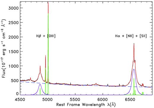
$Illustration of the spectral fitting for Mrk 290. The black solid line denotes the rest-frame SDSS spectrum. Purple and green lines represent the broad and narrow components of $\rm H\alpha$ and $\rm H\beta$, respectively. Red solid line shows the overall model.$

Figure 2.

Illustration of the spectral fitting for Mrk 290. The black solid line denotes the rest-frame SDSS spectrum. Purple and green lines represent the broad and narrow components of |$\rm H\alpha$| and |$\rm H\beta$|⁠, respectively. Red solid line shows the overall model.

Table 4.

SDSS spectral fitting results.

No.	Object	\|$\rm FWHM_{H\alpha ^b}$\|	\|$\rm FWHM_{H\beta ^b}$\|	\|$\log L_{\rm H\alpha ^b}$\|	\|$\log L_{\rm H\beta ^b}$\|	log L₅₁₀₀	\|$L_{\rm H\alpha ^b}/L_{\rm H\beta ^b}$\|	log (M_BH/M_\|$\odot$\|)
(1)	(2)	(3)	(4)	(5)	(6)	(7)	(8)	(9)
1	Mrk 1018	4152	6011	42.17	41.74	43.86	2.67	8.40
2	MCG 04-22-042	2062	2989	42.34	41.97	43.69	2.33	7.71
3	Mrk 705	2062	2039	42.03	41.57	43.38	2.88	7.22
4	RX J1007.1 + 2203	2092	2407	42.17	41.67	43.66	3.17	7.50
5	CBS 126	2639	2914	43.00	42.53	44.18	2.94	7.93
6	Mrk 141	3624	6672	41.91	41.39	43.51	3.31	8.31
7	Mrk 142	1494	1650	42.00	41.58	43.60	2.64	7.15
8	Ton 1388	2966	4004	44.11	43.60	45.27	3.25	8.75
9	SBS 1136 + 594	2637	3249	42.72	42.24	43.86	2.99	7.86
10	PG 1138 + 222	2246	2246	42.55	42.02	43.95	3.34	7.59
11	KUG 1141 + 371	6795	9049	41.82	41.36	43.28	2.83	8.46
12	Mrk 1310	2252	2717	41.31	40.92	42.75	2.46	7.16
13	RX J1209.8 + 3217	2019	2038	42.54	42.08	44.09	2.89	7.57
14	Mrk 50	4838	5837	41.78	41.33	43.07	2.83	7.98
15	Mrk 771	2800	3358	42.66	42.19	43.91	2.92	7.92
16	PG 1307 + 085	3650	4612	43.67	43.18	44.78	3.13	8.63
17	Ton 730	3009	3520	42.49	42.12	43.95	2.33	7.98
18	RX J1355.2 + 5612	1141	1192	42.67	42.16	44.16	3.22	7.14
19	Mrk 1392	4183	5371	42.29	41.83	43.60	2.91	8.17
20	Mrk 290	3612	4533	42.22	41.82	43.58	2.53	8.01
21	Mrk 493	1095	1095	41.71	41.29	43.41	2.63	7.51
22	KUG 1618 + 410	2045	2418	41.22	40.75	42.90	2.92	7.13
23	RX J1702.5 + 3247	2330	2442	43.27	42.82	44.70	2.82	8.03

No.	Object	\|$\rm FWHM_{H\alpha ^b}$\|	\|$\rm FWHM_{H\beta ^b}$\|	\|$\log L_{\rm H\alpha ^b}$\|	\|$\log L_{\rm H\beta ^b}$\|	log L₅₁₀₀	\|$L_{\rm H\alpha ^b}/L_{\rm H\beta ^b}$\|	log (M_BH/M_\|$\odot$\|)
(1)	(2)	(3)	(4)	(5)	(6)	(7)	(8)	(9)
1	Mrk 1018	4152	6011	42.17	41.74	43.86	2.67	8.40
2	MCG 04-22-042	2062	2989	42.34	41.97	43.69	2.33	7.71
3	Mrk 705	2062	2039	42.03	41.57	43.38	2.88	7.22
4	RX J1007.1 + 2203	2092	2407	42.17	41.67	43.66	3.17	7.50
5	CBS 126	2639	2914	43.00	42.53	44.18	2.94	7.93
6	Mrk 141	3624	6672	41.91	41.39	43.51	3.31	8.31
7	Mrk 142	1494	1650	42.00	41.58	43.60	2.64	7.15
8	Ton 1388	2966	4004	44.11	43.60	45.27	3.25	8.75
9	SBS 1136 + 594	2637	3249	42.72	42.24	43.86	2.99	7.86
10	PG 1138 + 222	2246	2246	42.55	42.02	43.95	3.34	7.59
11	KUG 1141 + 371	6795	9049	41.82	41.36	43.28	2.83	8.46
12	Mrk 1310	2252	2717	41.31	40.92	42.75	2.46	7.16
13	RX J1209.8 + 3217	2019	2038	42.54	42.08	44.09	2.89	7.57
14	Mrk 50	4838	5837	41.78	41.33	43.07	2.83	7.98
15	Mrk 771	2800	3358	42.66	42.19	43.91	2.92	7.92
16	PG 1307 + 085	3650	4612	43.67	43.18	44.78	3.13	8.63
17	Ton 730	3009	3520	42.49	42.12	43.95	2.33	7.98
18	RX J1355.2 + 5612	1141	1192	42.67	42.16	44.16	3.22	7.14
19	Mrk 1392	4183	5371	42.29	41.83	43.60	2.91	8.17
20	Mrk 290	3612	4533	42.22	41.82	43.58	2.53	8.01
21	Mrk 493	1095	1095	41.71	41.29	43.41	2.63	7.51
22	KUG 1618 + 410	2045	2418	41.22	40.75	42.90	2.92	7.13
23	RX J1702.5 + 3247	2330	2442	43.27	42.82	44.70	2.82	8.03

Notes: Column (1): identification number assigned in this paper. Column (2): NED name of the sample objects. Column (3): FWHM of the |$\rm H\alpha$| broad component. Column (4): FWHM of the |$\rm H\beta$| broad component. Column (5): logarithmic of the luminosity of the |$\rm H\alpha$| broad component in units of erg s⁻¹. Column (6): logarithmic of the luminosity of the |$\rm H\beta$| broad component in units of erg s⁻¹. Column (7): logarithmic of the 5100 Å monochromatic luminosity in units of erg s⁻¹. Column (8): broad-line Balmer decrement derived from |$L_{\rm H\alpha ^b}$|/|$L_{\rm H\beta ^b}$|⁠. Column (9): logarithmic of Black hole mass M_BH derived from |$\rm FWHM({H\beta ^b})$| and L₅₁₀₀ (Vestergaard & Peterson 2006) in units of M_|$\odot$|.

Table 4.

SDSS spectral fitting results.

No.	Object	\|$\rm FWHM_{H\alpha ^b}$\|	\|$\rm FWHM_{H\beta ^b}$\|	\|$\log L_{\rm H\alpha ^b}$\|	\|$\log L_{\rm H\beta ^b}$\|	log L₅₁₀₀	\|$L_{\rm H\alpha ^b}/L_{\rm H\beta ^b}$\|	log (M_BH/M_\|$\odot$\|)
(1)	(2)	(3)	(4)	(5)	(6)	(7)	(8)	(9)
1	Mrk 1018	4152	6011	42.17	41.74	43.86	2.67	8.40
2	MCG 04-22-042	2062	2989	42.34	41.97	43.69	2.33	7.71
3	Mrk 705	2062	2039	42.03	41.57	43.38	2.88	7.22
4	RX J1007.1 + 2203	2092	2407	42.17	41.67	43.66	3.17	7.50
5	CBS 126	2639	2914	43.00	42.53	44.18	2.94	7.93
6	Mrk 141	3624	6672	41.91	41.39	43.51	3.31	8.31
7	Mrk 142	1494	1650	42.00	41.58	43.60	2.64	7.15
8	Ton 1388	2966	4004	44.11	43.60	45.27	3.25	8.75
9	SBS 1136 + 594	2637	3249	42.72	42.24	43.86	2.99	7.86
10	PG 1138 + 222	2246	2246	42.55	42.02	43.95	3.34	7.59
11	KUG 1141 + 371	6795	9049	41.82	41.36	43.28	2.83	8.46
12	Mrk 1310	2252	2717	41.31	40.92	42.75	2.46	7.16
13	RX J1209.8 + 3217	2019	2038	42.54	42.08	44.09	2.89	7.57
14	Mrk 50	4838	5837	41.78	41.33	43.07	2.83	7.98
15	Mrk 771	2800	3358	42.66	42.19	43.91	2.92	7.92
16	PG 1307 + 085	3650	4612	43.67	43.18	44.78	3.13	8.63
17	Ton 730	3009	3520	42.49	42.12	43.95	2.33	7.98
18	RX J1355.2 + 5612	1141	1192	42.67	42.16	44.16	3.22	7.14
19	Mrk 1392	4183	5371	42.29	41.83	43.60	2.91	8.17
20	Mrk 290	3612	4533	42.22	41.82	43.58	2.53	8.01
21	Mrk 493	1095	1095	41.71	41.29	43.41	2.63	7.51
22	KUG 1618 + 410	2045	2418	41.22	40.75	42.90	2.92	7.13
23	RX J1702.5 + 3247	2330	2442	43.27	42.82	44.70	2.82	8.03

No.	Object	\|$\rm FWHM_{H\alpha ^b}$\|	\|$\rm FWHM_{H\beta ^b}$\|	\|$\log L_{\rm H\alpha ^b}$\|	\|$\log L_{\rm H\beta ^b}$\|	log L₅₁₀₀	\|$L_{\rm H\alpha ^b}/L_{\rm H\beta ^b}$\|	log (M_BH/M_\|$\odot$\|)
(1)	(2)	(3)	(4)	(5)	(6)	(7)	(8)	(9)
1	Mrk 1018	4152	6011	42.17	41.74	43.86	2.67	8.40
2	MCG 04-22-042	2062	2989	42.34	41.97	43.69	2.33	7.71
3	Mrk 705	2062	2039	42.03	41.57	43.38	2.88	7.22
4	RX J1007.1 + 2203	2092	2407	42.17	41.67	43.66	3.17	7.50
5	CBS 126	2639	2914	43.00	42.53	44.18	2.94	7.93
6	Mrk 141	3624	6672	41.91	41.39	43.51	3.31	8.31
7	Mrk 142	1494	1650	42.00	41.58	43.60	2.64	7.15
8	Ton 1388	2966	4004	44.11	43.60	45.27	3.25	8.75
9	SBS 1136 + 594	2637	3249	42.72	42.24	43.86	2.99	7.86
10	PG 1138 + 222	2246	2246	42.55	42.02	43.95	3.34	7.59
11	KUG 1141 + 371	6795	9049	41.82	41.36	43.28	2.83	8.46
12	Mrk 1310	2252	2717	41.31	40.92	42.75	2.46	7.16
13	RX J1209.8 + 3217	2019	2038	42.54	42.08	44.09	2.89	7.57
14	Mrk 50	4838	5837	41.78	41.33	43.07	2.83	7.98
15	Mrk 771	2800	3358	42.66	42.19	43.91	2.92	7.92
16	PG 1307 + 085	3650	4612	43.67	43.18	44.78	3.13	8.63
17	Ton 730	3009	3520	42.49	42.12	43.95	2.33	7.98
18	RX J1355.2 + 5612	1141	1192	42.67	42.16	44.16	3.22	7.14
19	Mrk 1392	4183	5371	42.29	41.83	43.60	2.91	8.17
20	Mrk 290	3612	4533	42.22	41.82	43.58	2.53	8.01
21	Mrk 493	1095	1095	41.71	41.29	43.41	2.63	7.51
22	KUG 1618 + 410	2045	2418	41.22	40.75	42.90	2.92	7.13
23	RX J1702.5 + 3247	2330	2442	43.27	42.82	44.70	2.82	8.03

Notes: Column (1): identification number assigned in this paper. Column (2): NED name of the sample objects. Column (3): FWHM of the |$\rm H\alpha$| broad component. Column (4): FWHM of the |$\rm H\beta$| broad component. Column (5): logarithmic of the luminosity of the |$\rm H\alpha$| broad component in units of erg s⁻¹. Column (6): logarithmic of the luminosity of the |$\rm H\beta$| broad component in units of erg s⁻¹. Column (7): logarithmic of the 5100 Å monochromatic luminosity in units of erg s⁻¹. Column (8): broad-line Balmer decrement derived from |$L_{\rm H\alpha ^b}$|/|$L_{\rm H\beta ^b}$|⁠. Column (9): logarithmic of Black hole mass M_BH derived from |$\rm FWHM({H\beta ^b})$| and L₅₁₀₀ (Vestergaard & Peterson 2006) in units of M_|$\odot$|.

3.4 Estimation of intrinsic dust extinction and black hole mass

The intrinsic dust extinction in our sample AGN is estimated from the broad-line Balmer decrement, which is derived from the flux ratio of the broad components of |$\rm H{\alpha }$| and |$\rm H{\beta }$|⁠. The intrinsic value of |$\rm H{\alpha }$|/|$\rm H{\beta }$| of AGN with no dust reddening has been a topic of debate (e.g. Dong et al. 2005; La Mura et al. 2007; Dong et al. 2008; Schnorr-Müller et al. 2016; Gaskell 2017). In this work, we adopt an intrinsic |$\rm H{\alpha }$|/|$\rm H{\beta }$| value of 3.06 derive by Dong et al. (2008) based on a sample of 446 blue AGNs, which is verified later by Baron et al. (2016) with a much larger AGN sample and has been employed in various studies (e.g. Wang et al. 2009b; Grupe et al. 2010; Liu et al. 2016). The colour excess is derived as

\begin{eqnarray*} E(B-V)=2.12\log \frac{L_{\rm H\alpha ^b}/L_{\rm H\beta ^b}}{3.06} \end{eqnarray*}

(1)

by using the Small Magellanic Cloud (SMC) extinction curve, which is suggested to be applicable in AGN (e.g. Hopkins et al. 2004; Czerny 2007; Li 2007; Krawczyk et al. 2015, see Section 6.1 for the discussion of using other extinction curves). The derived broad-line Balmer decrements |$L_{\rm H\alpha ^b}/L_{\rm H\beta ^b}$| are listed in Table 4, and their distribution is plotted in Fig. 3. The Balmer decrements are around 2.2–3.4, indicating little or no dust extinction in most of the sample objects (⁠|$\rm H{\alpha }$|/|$\rm H{\beta }$| ≤ 3.06), except for a few cases where some moderate extinction might be present. For the six objects with |$\rm H{\alpha }$|/|$\rm H{\beta }$|>3.06, the intrinsic continuum fluxes at the six UVOT filters are derived by correcting for the excess reddening effect from the E(B − V) derived above, using the idl code smc_unred.pro.⁸

Figure 3.

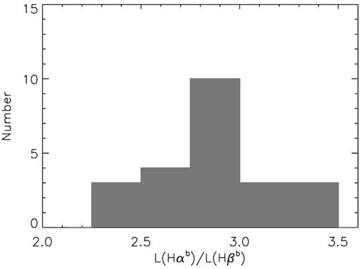
The distribution of the broad-line Balmer decrements for the sample.

The BH masses of AGN can be estimated using the spectral measurements based on the virial method (e.g. Kaspi et al. 2000; Wang et al. 2009a). In this work, the BH masses are estimated using the FWHMs of the |$\rm H{\beta }$| broad component and monochromatic luminosity at 5100 Å (equation 5 in Vestergaard & Peterson 2006). It should be noted that the black hole mass estimated in this way is indirect and subject to systematics as large as ∼0.3 dex (e.g. Gebhardt et al. 2000; Greene & Ho 2006; Grier et al. 2013, the effect on our results is discussed in Section 4.2). The values of the black hole masses are also listed in Table 4, and the distribution is shown in Fig. 4. The black hole masses lie in the range of 10⁷–10⁹|$\, \mathrm{M}_{\odot }$| with a median around 10⁸|$\, \mathrm{M}_{\odot }$|⁠.

Figure 4.

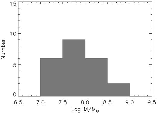
The distribution of the black hole masses for the sample.

4 MODELLING THE OPTICAL/UV CONTINUUM

4.1 Optical/UV spectral slopes

Assuming the optical/UV continuum of an AGN (at a redshift z) is radiated from a geometrically thin, optically thick disc, the rest-frame luminosity at the frequency ν is calculated as

\begin{eqnarray*} \nu L_{\nu } &= \nu _0F_{\nu _0}\times \frac{2\pi d_{\rm L}^2}{\cos {i}}, \end{eqnarray*}

(2)

\begin{eqnarray*} \nu &= \nu _0(1+z), \end{eqnarray*}

(3)

where |$F_{\nu _0}$| is the flux density (in units of |$\rm erg \ cm^{-2} \ s^{-1} \ Hz^{-1}$|⁠) observed at a frequency ν₀ in the observer’s frame. d_L is the luminosity distance. i is the viewing angle to the norm of the accretion disc (i = 0° for face-on). In this work, we assume i = 30°, a typical value for type 1 AGN as commonly adopted and also consistent with polarization measurement (Marin 2014). It should be noted that the optical/UV continuum spectral shapes derived below are independent of the assumption of the disc inclination. The effect of varying the inclination on our results is also discussed below.

First, a simple power-law model is used to fit the optical/UV spectra. The fitted slopes α_opt-UV are listed in Table 6. Fig. 5 shows the distribution, which lie in the range of −1.0 to +0.3 with a median of −0.39. It shows that most of the sources have a shallower α_opt-UV than that of the SSD (+1/3), consistent with most of the previous results. Considering that the host galaxy contamination and possible dust reddening have been largely eliminated in this work, their effects on the observed spectral slopes are considered to be small, and hence cannot account for the reddening of the optical/UV spectra (see Section 6.1 for discussion on the systematics). Here, we consider that the derived continua are intrinsic emission from the AGN. As mentioned above, a shallower optical/UV spectral slope is at odds with that predicted from the SSD model.

Figure 5.

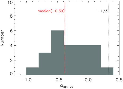
The distribution of the optical/UV spectral index α_opt-UV. The red dotted line represents α_opt-UV = −0.39 (the median). The black dotted line represents α_opt-UV = +1/3 (the SSD prediction).

4.2 Accretion disc model with non-standard radial temperature profile

In this work, an alternative approach is adopted as an attempt to reconcile the observation with theoretical models of accretion discs. We consider that the observed optical/UV spectra originate intrinsically from a realistic accretion disc whose radial profile of the effective temperature deviates from the SSD solution. For this purpose, a generalized radial profile of the effective temperature is assumed,

\begin{eqnarray*} T_{\rm eff}(R) = T_{\rm eff}(R_{\rm in})\times \left(\frac{R}{R_{\rm in}}\right)^{-p} \end{eqnarray*}

(4)

where T_eff(R_in) is the effective temperature at the inner disc radius R_in and the index p a free parameter. Such a model is sometimes dubbed as p-free disc model in the literature (e.g. Kubota & Makishima 2004; Kubota et al. 2005; Ai et al. 2011). This model was first introduced in the studies of black hole X-ray binaries (XRBs) to verify the disc solution in outbursts (Mineshige et al. 1994; Hirano et al. 1995). Other values of p deviating from the SSD value 0.75 have physical meanings. For instance, under the assumption of local thermodynamic equilibrium (LTE), |$T_{\rm eff}(R)\propto M_{\rm BH}^{1/4}\dot{M}^{1/4}R^{-3/4}$| (e.g. Frank et al. 2002; Kato et al. 2008), a non-standard radial temperature profile may result from a radius-dependent mass flow rate distribution (⁠|$\dot{M}(R)\propto R^{3-4p}$|⁠, where p ≠ 0.75), in contrast to the constant (R-independent) |$\dot{M}$| in the standard disc formalism (p = 0.75). In reality, this may well be the case for an realistic accretion disc with mass evaporation/outflow or condensation.

The total disc luminosity at a frequency ν can be calculated as the integral of the local blackbody radiation from the inner disc radius R_in to the outmost disc R_out

\begin{eqnarray*} L_{\nu }=2\int _{R_{\rm in}}^{R_{\rm out}}\pi B_{\nu }(R)2\pi R\mathrm{ d}R \end{eqnarray*}

(5)

in which

\begin{eqnarray*} &B_{\nu }(R)=\frac{2 \rm h \nu ^{3} }{{\rm c^2}{f_{\rm col}^4}} \frac{1}{\mathrm{ e}^{{\rm h} \nu /{{\rm k_{B}}T(R)}}-1}, \end{eqnarray*}

(6)

\begin{eqnarray*} &T(R)=f_{\rm col}T_{\rm eff}(R) , \end{eqnarray*}

(7)

where T(R) is the color temperature and f_col represents the electron scattering correction to the pure local blackbody radiation (also refer to hardening factor, e.g. Shimura & Takahara 1995; Salvesen et al. 2013; Davis & EI-Abd 2019). For XRBs, a typical value of ∼1.7 is often used (Shimura & Takahara 1995). Little is known for the hardening factor for AGN, however. The characteristic disc temperature in AGN is about two orders of magnitude lower than that in XRBs and the colour correction is suggested to be 1.0–1.6 in some studies (e.g. Czerny et al. 2011; You et al. 2016). Here, we adopt f_col = 1, as in some similar previous studies (e.g. Vasudevan & Fabian 2007, 2009). For a disc extending all the way to the innermost stable circular orbit, the inner disc radius R_in is determined by the black hole spin (a_*), from ∼R_g (=GM_BH/c² is the gravitational radius) for a corotating disc around an extremely spinning BH (a_* = 0.99) to 3R_s (R_s = 2R_g, the Schwarzschild radius) for a non-spinning BH (a_* = 0), and 9R_g for a retrograde-rotating disc around an extremely spinning BH (a_* = −1). As a common practice here a non-spinning BH is assumed following Vasudevan & Fabian (2007) and thus R_in = 6R_g. R_out is the outer radius of the disc, which is determined by the self-gravity of the accretion disc (Laor & Netzer 1989) and set to a typical value 3000R_s.⁹ The black hole masses derived from the optical spectral parameters (see Section 3.4) are used to calculate R_g.

In this model, the inner disc temperature T_eff(R_in) and index p in equation (4) are free parameters. The value of p allowed in the fitting is set to a reasonable range of [0.45, 0.85], considering the limits in the classical accretion theory (p = 0.5 in ‘slim’ disc and 0.75 in SSD) and possible uncertainty in the spectral fitting procedure caused by other parameters such as black hole mass (see below). The idl routine mpfit (Markwardt 2009), which employs the Levenberg–Marquardt least-squares method, is used to fit the optical/UV spectra obtained above with the p-free disc model. For most of the objects, the model can fit the optical/UV data reasonably well. The best-fitting values of p and T_eff(R_in) are listed in Table 6. The measured AGN optical/UV luminosities and the best-fitting disk models are shown in Fig. 6.

The SEDs for our sample, including the measured luminosities and spectral models in optical/UV and X-ray bands. Red dots represent the measured luminosities in the six UVOT filters. Black crosses represent the X-ray luminosities obtained by XRT instrument. The spectral model components are denoted by dashed lines in different colours. The red dashed line represents the p-free disc model. The green dashed line represents the blackbody model (if required). The blue dashed line represents the power-law model, which is extrapolated by an exponential cutoff at both ends. The sum of all models is represented by a pink solid line. The data and models are in the source rest-frame.

Figure 6.

The SEDs for our sample, including the measured luminosities and spectral models in optical/UV and X-ray bands. Red dots represent the measured luminosities in the six UVOT filters. Black crosses represent the X-ray luminosities obtained by XRT instrument. The spectral model components are denoted by dashed lines in different colours. The red dashed line represents the p-free disc model. The green dashed line represents the blackbody model (if required). The blue dashed line represents the power-law model, which is extrapolated by an exponential cutoff at both ends. The sum of all models is represented by a pink solid line. The data and models are in the source rest-frame.

The above fitted p and T_eff(R_in) values are obtained by assuming a specific set of parameters of the BH and the accretion disc, which might deviate in reality. Moreover, the black hole masses estimated in Section 3.4 from the single-epoch optical spectra are subject to systematic uncertainties as large as ∼0.3 dex. To investigate the systematics of the fitted p and T_eff(R_in) values caused by these uncertainties, the above fitting procedure is repeated for 5000 times using various combinations of the values of these parameters which are drawn randomly from reasonable ranges in the parameter space of M_BH, a_*, and i. Specifically, M_BH is drawn from a Gaussian distribution of log (M_BH) with a standard deviation σ = 0.3, and i and a_* from a uniform distribution in the [0°–60°] and [−0.99 to +0.99] ranges, respectively. The 1σ error of p and T_eff(R_in) is derived from the simulated distribution and given in Table 6.

Fig. 7 shows the distribution of the best-fitting indices of p. The majority lie between 0.5 and 0.75 with a median of 0.63, suggesting a flatter radial temperature profile than that of the SSD model (0.75) in most of the sample objects. Theoretically, the slope of the power-law regime of an emergent disc spectrum in optical/UV band can be determined by the radial temperature profile of the disc, and thus a relation between the two can be predicted, as α_opt-UV = 3 − 2/p (e.g. Gaskell 2008). The relationship between the obtained p values and α_opt-UV is shown in Fig. 8, which is found to be consistent with the theoretical relation for most of the objects. In these sources, the UVOT data mainly sampled the power-law portion of the emergent disc spectra. The value of p is mainly determined by α_opt-UV and has a weak dependence on the black hole mass (thus has a small uncertainty). The Spearman’s rank test confirms a strong correlation between these two parameters (ρ_s = 0.63 and P = 1.320 × 10⁻³). Fig. 8 also reveals a few outliers with rather redder spectra. By examining, the spectral fits it is clear that for these sources the UVOT data sampled mostly the Wien rather than the power-law regime of the spectrum (this also leads to a strong dependence of p on the black hole mass and a large uncertainty therein). Among these, KUG 1141 + 371 is an extreme case with the shallowest spectral slope (α_opt-UV = −0.84), while the index is fitted to be p ≈ 0.74, indicating a radial temperature profile very close to that of the SSD. The result shows that in some AGN the shallower optical/UV slopes may simply be caused by the fact that the peak or the high-energy turnover of the disc spectrum is observed, which is expected in AGN with high BH mass M_BH and relatively low Eddington ratio λ_Edd (see Fig. 6 for the SED fitting for KUG 1141 + 371).

Figure 7.

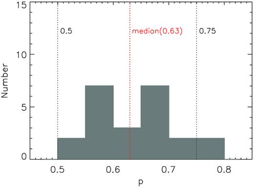
The distribution of the radial temperature power-law index p, obtained from the optical/UV spectral fitting using the p-free disc model. The two black dotted lines represent p = 0.5 (‘slim’ disc solution) and p = 0.75 (SSD solution). The red dotted line represents p = 0.63 (the median).

Figure 8.

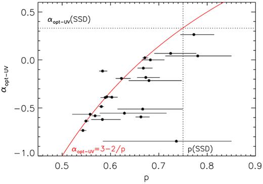
Power-law index of the radial temperature profile p versus optical/UV spectra slope α_opt-UV. The vertical dotted line represents p = 0.75 (SSD solution). The horizontal dotted line represents α_opt-UV = +1/3 (SSD prediction). The red solid line represents the theoretical relation of p and α_opt-UV assuming UVOT data sample the power-law regime of the disc spectrum. The error of p are given in 1σ.

5 BROAD-BAND SED AND BOLOMETRIC CORRECTION FACTORS

It has been shown above that the optical/UV spectra in most of our AGN can well be reproduced by emission from accretion discs with a flattened radial temperature profile. As a result, such a disc produces relatively lower emission in the EUV band than that previously predicted for an SSD model with the F_ν ∝ ν^+1/3 spectrum. This energy band is thought to be where the disc emission peaks, and thus contains a substantial fraction of the bolometric luminosity. In the rest of the paper, we investigate the broad-band SED for our sample AGN assuming that a non-SSD radial temperature profile may operate in accretion discs.

Aside from the optical/UV band, another dominant emission bandpass is X-ray. In this section, we first model the X-ray emission by making use of the simultaneous Swift/XRT observations. Then, the broad-band SEDs are constructed and the bolometric luminosities are derived. Finally, the bolometric correction factors are studied for the X-ray and optical bands.

5.1 The 0.3–10 keV X-ray band

We make use of the xspec software (Arnaud 1996, version 12.9.1) to model the XRT spectra of our sample objects in the observed 0.3–10 keV energy band. An absorbed power-law model (wabs×powerlaw) with a free absorption column density (N_H) is fitted to the spectra at first, and the fitted N_H do not show evidence for excess absorption above the Galactic value. We thus fix the absorption column densities at the Galactic value for better constraining of the spectral parameters. The spectra of six AGN can be well fitted with a simple absorbed power-law model. In other 16 sources, a possible soft excess component below 2 keV is indicated in the fitting residuals when the model is fitted to the 2–10 keV data and is extrapolated below 2 keV. We thus add a blackbody component in the model (wabs×(bbody + powerlaw)), whose addition is justified by using the F-test and an acceptance P-value of P < 0.05 is adopted. For these objects, an absorbed power-law plus a soft X-ray excess model is found to better describe the X-ray spectra. The temperature of the soft excess is found to be T_bb ≈ 0.1–0.2 keV, consistent with the typcial values in AGN. In the remaining source RX J1209.8 + 3217, a distinct feature is noticed, with a possible absorption around 1–2 keV. A power-law model plus an ionized absorption component (wabs×absori×powerlaw) with their photon indices tied with each other gives a satisfactory fit. The results of the X-ray spectral analysis are summarized in Table 5 (the errors are given in |$90{{\ \rm per\ cent}}$| confidence interval). We note that the reflection component which is often observed in Seyfert galaxies should have a negligible effect to the determination of X-ray power-law continuum in this work, as the practical energy range of the XRT spectra for our sample objects are all below 8 keV.

Table 5.

Spectral analysis of XRT spectra.

No.	Object	Model	\|$N_{\rm H}^{\rm Gal}$\|	Γ_X	T_bb	log F_2-10	χ²/ν	Count rates
(1)	(2)	(3)	(4)	(5)	(6)	(7)	(8)	(9)
1	Mrk 1018	(b)	2.43	\|$1.84_{-0.13}^{+0.13}$\|	\|$0.12_{-0.04}^{+0.03}$\|	\|$-10.91_{-0.05}^{+0.05}$\|	37/53	0.302 ± 0.008
2	MCG 04-22-042	(b)	3.12	\|$1.78_{-0.10}^{+0.10}$\|	\|$0.12_{-0.04}^{+0.03}$\|	\|$-10.90_{-0.04}^{+0.03}$\|	78/83	0.282 ± 0.006
3	Mrk 705	(b)	3.22	\|$1.72_{-0.27}^{+0.26}$\|	\|$0.15_{-0.03}^{+0.02}$\|	\|$-11.11_{-0.09}^{+0.08}$\|	35/33	0.473 ± 0.020
4	RX J1007.1 + 2203	(b)	2.60	\|$1.69_{-0.40}^{+0.39}$\|	\|$0.12_{-0.02}^{+0.01}$\|	\|$-12.24_{-0.14}^{+0.11}$\|	15/13	0.037 ± 0.002
5	CBS 126	(b)	0.97	\|$1.71_{-0.21}^{+0.21}$\|	\|$0.09_{-0.01}^{+0.01}$\|	\|$-11.65_{-0.09}^{+0.08}$\|	18/19	0.136 ± 0.005
6	Mrk 141	(b)	1.18	\|$1.69_{-0.14}^{+0.13}$\|	\|$0.08_{-0.03}^{+0.04}$\|	\|$-11.59_{-0.06}^{+0.06}$\|	15/28	0.105 ± 0.004
7	Mrk 142	(b)	1.18	\|$1.74_{-0.62}^{+0.62}$\|	\|$0.13_{-0.02}^{+0.01}$\|	\|$-11.38_{-0.23}^{+0.14}$\|	15/17	0.201 ± 0.008
8	Ton 1388	(a)	1.38	\|$2.24_{-0.07}^{+0.07}$\|	–	\|$-11.50_{-0.05}^{+0.04}$\|	45/42	0.255 ± 0.007
9	SBS 1136 + 594	(b)	0.94	\|$1.64_{-0.08}^{+0.08}$\|	\|$0.12_{-0.01}^{+0.01}$\|	\|$-11.10_{-0.03}^{+0.03}$\|	108/104	0.370 ± 0.006
10	PG 1138 + 222	(a)	2.02	\|$1.92_{-0.07}^{+0.07}$\|	–	\|$-11.10_{-0.04}^{+0.04}$\|	43/51	0.364 ± 0.009
11	KUG 1141 + 371	(a)	1.65	\|$1.48_{-0.15}^{+0.15}$\|	–	\|$-11.39_{-0.09}^{+0.08}$\|	13/12	0.132 ± 0.007
12	Mrk 1310	(b)	2.50	\|$1.33_{-0.33}^{+0.30}$\|	\|$0.18_{-0.03}^{+0.03}$\|	\|$-11.31_{-0.09}^{+0.08}$\|	10/17	0.135 ± 0.006
13	RX J1209.8 + 3217	(c)	1.24	\|$2.57_{-0.06}^{+0.15}$\|	–	\|$-12.81_{-0.11}^{+0.06}$\|	9/7	0.017 ± 0.001
14	Mrk 50	(a)	1.58	\|$1.79_{-0.05}^{+0.05}$\|	–	\|$-11.06_{-0.03}^{+0.03}$\|	73/82	0.384 ± 0.008
15	Mrk 771	(b)	2.75	\|$2.04_{-0.13}^{+0.13}$\|	\|$0.09_{-0.03}^{+0.02}$\|	\|$-11.44_{-0.05}^{+0.05}$\|	64/53	0.245 ± 0.006
16	PG 1307 + 085	(b)	2.21	\|$1.71_{-0.16}^{+0.16}$\|	\|$0.12_{-0.03}^{+0.02}$\|	\|$-11.45_{-0.05}^{+0.05}$\|	53/49	0.146 ± 0.006
17	Ton 730	(a)	1.11	\|${2.17}_{-0.08}^{+0.08}$\|	–	\|$-11.80_{-0.05}^{+0.05}$\|	68/48	0.119 ± 0.003
18	RX J1355.2 + 5612	(b)	1.02	\|$1.85_{-0.58}^{+0.54}$\|	\|${0.10}_{-0.01}^{+0.01}$\|	\|$-11.99_{-0.21}^{+0.18}$\|	10/9	0.078 ± 0.004
19	Mrk 1392	(b)	3.80	\|$1.82_{-0.11}^{+0.11}$\|	\|$0.10_{-0.02}^{+0.02}$\|	\|$-11.26_{-0.05}^{+0.04}$\|	54/52	0.253 ± 0.006
20	Mrk 290	(b)	1.76	\|$1.40_{-0.11}^{+0.11}$\|	\|$0.09_{-0.02}^{+0.02}$\|	\|$-11.13_{-0.05}^{+0.04}$\|	58/43	0.237 ± 0.007
21	Mrk 493	(b)	2.11	\|$2.12_{-0.18}^{+0.17}$\|	\|$0.14_{-0.03}^{+0.03}$\|	\|$-11.62_{-0.06}^{+0.06}$\|	29/45	0.197 ± 0.005
22	KUG 1618 + 410	(a)	0.84	\|$1.64_{-0.46}^{+0.51}$\|	–	\|$-11.86_{-0.26}^{+0.21}$\|	1.5/1	0.032 ± 0.004
23	RX J1702.5 + 3247	(b)	1.98	\|$2.50_{-0.18}^{+0.19}$\|	\|$0.10_{-0.02}^{+0.01}$\|	\|$-11.90_{-0.07}^{+0.06}$\|	40/46	0.170 ± 0.004

No.	Object	Model	\|$N_{\rm H}^{\rm Gal}$\|	Γ_X	T_bb	log F_2-10	χ²/ν	Count rates
(1)	(2)	(3)	(4)	(5)	(6)	(7)	(8)	(9)
1	Mrk 1018	(b)	2.43	\|$1.84_{-0.13}^{+0.13}$\|	\|$0.12_{-0.04}^{+0.03}$\|	\|$-10.91_{-0.05}^{+0.05}$\|	37/53	0.302 ± 0.008
2	MCG 04-22-042	(b)	3.12	\|$1.78_{-0.10}^{+0.10}$\|	\|$0.12_{-0.04}^{+0.03}$\|	\|$-10.90_{-0.04}^{+0.03}$\|	78/83	0.282 ± 0.006
3	Mrk 705	(b)	3.22	\|$1.72_{-0.27}^{+0.26}$\|	\|$0.15_{-0.03}^{+0.02}$\|	\|$-11.11_{-0.09}^{+0.08}$\|	35/33	0.473 ± 0.020
4	RX J1007.1 + 2203	(b)	2.60	\|$1.69_{-0.40}^{+0.39}$\|	\|$0.12_{-0.02}^{+0.01}$\|	\|$-12.24_{-0.14}^{+0.11}$\|	15/13	0.037 ± 0.002
5	CBS 126	(b)	0.97	\|$1.71_{-0.21}^{+0.21}$\|	\|$0.09_{-0.01}^{+0.01}$\|	\|$-11.65_{-0.09}^{+0.08}$\|	18/19	0.136 ± 0.005
6	Mrk 141	(b)	1.18	\|$1.69_{-0.14}^{+0.13}$\|	\|$0.08_{-0.03}^{+0.04}$\|	\|$-11.59_{-0.06}^{+0.06}$\|	15/28	0.105 ± 0.004
7	Mrk 142	(b)	1.18	\|$1.74_{-0.62}^{+0.62}$\|	\|$0.13_{-0.02}^{+0.01}$\|	\|$-11.38_{-0.23}^{+0.14}$\|	15/17	0.201 ± 0.008
8	Ton 1388	(a)	1.38	\|$2.24_{-0.07}^{+0.07}$\|	–	\|$-11.50_{-0.05}^{+0.04}$\|	45/42	0.255 ± 0.007
9	SBS 1136 + 594	(b)	0.94	\|$1.64_{-0.08}^{+0.08}$\|	\|$0.12_{-0.01}^{+0.01}$\|	\|$-11.10_{-0.03}^{+0.03}$\|	108/104	0.370 ± 0.006
10	PG 1138 + 222	(a)	2.02	\|$1.92_{-0.07}^{+0.07}$\|	–	\|$-11.10_{-0.04}^{+0.04}$\|	43/51	0.364 ± 0.009
11	KUG 1141 + 371	(a)	1.65	\|$1.48_{-0.15}^{+0.15}$\|	–	\|$-11.39_{-0.09}^{+0.08}$\|	13/12	0.132 ± 0.007
12	Mrk 1310	(b)	2.50	\|$1.33_{-0.33}^{+0.30}$\|	\|$0.18_{-0.03}^{+0.03}$\|	\|$-11.31_{-0.09}^{+0.08}$\|	10/17	0.135 ± 0.006
13	RX J1209.8 + 3217	(c)	1.24	\|$2.57_{-0.06}^{+0.15}$\|	–	\|$-12.81_{-0.11}^{+0.06}$\|	9/7	0.017 ± 0.001
14	Mrk 50	(a)	1.58	\|$1.79_{-0.05}^{+0.05}$\|	–	\|$-11.06_{-0.03}^{+0.03}$\|	73/82	0.384 ± 0.008
15	Mrk 771	(b)	2.75	\|$2.04_{-0.13}^{+0.13}$\|	\|$0.09_{-0.03}^{+0.02}$\|	\|$-11.44_{-0.05}^{+0.05}$\|	64/53	0.245 ± 0.006
16	PG 1307 + 085	(b)	2.21	\|$1.71_{-0.16}^{+0.16}$\|	\|$0.12_{-0.03}^{+0.02}$\|	\|$-11.45_{-0.05}^{+0.05}$\|	53/49	0.146 ± 0.006
17	Ton 730	(a)	1.11	\|${2.17}_{-0.08}^{+0.08}$\|	–	\|$-11.80_{-0.05}^{+0.05}$\|	68/48	0.119 ± 0.003
18	RX J1355.2 + 5612	(b)	1.02	\|$1.85_{-0.58}^{+0.54}$\|	\|${0.10}_{-0.01}^{+0.01}$\|	\|$-11.99_{-0.21}^{+0.18}$\|	10/9	0.078 ± 0.004
19	Mrk 1392	(b)	3.80	\|$1.82_{-0.11}^{+0.11}$\|	\|$0.10_{-0.02}^{+0.02}$\|	\|$-11.26_{-0.05}^{+0.04}$\|	54/52	0.253 ± 0.006
20	Mrk 290	(b)	1.76	\|$1.40_{-0.11}^{+0.11}$\|	\|$0.09_{-0.02}^{+0.02}$\|	\|$-11.13_{-0.05}^{+0.04}$\|	58/43	0.237 ± 0.007
21	Mrk 493	(b)	2.11	\|$2.12_{-0.18}^{+0.17}$\|	\|$0.14_{-0.03}^{+0.03}$\|	\|$-11.62_{-0.06}^{+0.06}$\|	29/45	0.197 ± 0.005
22	KUG 1618 + 410	(a)	0.84	\|$1.64_{-0.46}^{+0.51}$\|	–	\|$-11.86_{-0.26}^{+0.21}$\|	1.5/1	0.032 ± 0.004
23	RX J1702.5 + 3247	(b)	1.98	\|$2.50_{-0.18}^{+0.19}$\|	\|$0.10_{-0.02}^{+0.01}$\|	\|$-11.90_{-0.07}^{+0.06}$\|	40/46	0.170 ± 0.004

Notes: Column (1): identification number assigned in this paper. Column (2): NED name of the sample objects. Column (3): the xspec models used: (a) wabs×powerlaw (b) wabs×(bbody + powerlaw) (c) wabs×absori×powerlaw. Column (4): the neutral hydrogen column density |$N_{\rm H}^{\rm Gal}$| used in wabs in units of 10²⁰ cm⁻². Column (5): the hard X-ray photon index Γ_X in powerlaw. Column (6): the blackbody temperature in units of keV in bbody. Column (7): logarithmic of the observed 2−10 keV flux in units of erg cm⁻² s⁻¹. Column (8): the goodness of fit for the model. Column (9): the XRT count rates in the observed 0.3−10 keV band in units of counts s⁻¹. The errors are given in 90 per cent confidence interval.

Table 5.

Spectral analysis of XRT spectra.

No.	Object	Model	\|$N_{\rm H}^{\rm Gal}$\|	Γ_X	T_bb	log F_2-10	χ²/ν	Count rates
(1)	(2)	(3)	(4)	(5)	(6)	(7)	(8)	(9)
1	Mrk 1018	(b)	2.43	\|$1.84_{-0.13}^{+0.13}$\|	\|$0.12_{-0.04}^{+0.03}$\|	\|$-10.91_{-0.05}^{+0.05}$\|	37/53	0.302 ± 0.008
2	MCG 04-22-042	(b)	3.12	\|$1.78_{-0.10}^{+0.10}$\|	\|$0.12_{-0.04}^{+0.03}$\|	\|$-10.90_{-0.04}^{+0.03}$\|	78/83	0.282 ± 0.006
3	Mrk 705	(b)	3.22	\|$1.72_{-0.27}^{+0.26}$\|	\|$0.15_{-0.03}^{+0.02}$\|	\|$-11.11_{-0.09}^{+0.08}$\|	35/33	0.473 ± 0.020
4	RX J1007.1 + 2203	(b)	2.60	\|$1.69_{-0.40}^{+0.39}$\|	\|$0.12_{-0.02}^{+0.01}$\|	\|$-12.24_{-0.14}^{+0.11}$\|	15/13	0.037 ± 0.002
5	CBS 126	(b)	0.97	\|$1.71_{-0.21}^{+0.21}$\|	\|$0.09_{-0.01}^{+0.01}$\|	\|$-11.65_{-0.09}^{+0.08}$\|	18/19	0.136 ± 0.005
6	Mrk 141	(b)	1.18	\|$1.69_{-0.14}^{+0.13}$\|	\|$0.08_{-0.03}^{+0.04}$\|	\|$-11.59_{-0.06}^{+0.06}$\|	15/28	0.105 ± 0.004
7	Mrk 142	(b)	1.18	\|$1.74_{-0.62}^{+0.62}$\|	\|$0.13_{-0.02}^{+0.01}$\|	\|$-11.38_{-0.23}^{+0.14}$\|	15/17	0.201 ± 0.008
8	Ton 1388	(a)	1.38	\|$2.24_{-0.07}^{+0.07}$\|	–	\|$-11.50_{-0.05}^{+0.04}$\|	45/42	0.255 ± 0.007
9	SBS 1136 + 594	(b)	0.94	\|$1.64_{-0.08}^{+0.08}$\|	\|$0.12_{-0.01}^{+0.01}$\|	\|$-11.10_{-0.03}^{+0.03}$\|	108/104	0.370 ± 0.006
10	PG 1138 + 222	(a)	2.02	\|$1.92_{-0.07}^{+0.07}$\|	–	\|$-11.10_{-0.04}^{+0.04}$\|	43/51	0.364 ± 0.009
11	KUG 1141 + 371	(a)	1.65	\|$1.48_{-0.15}^{+0.15}$\|	–	\|$-11.39_{-0.09}^{+0.08}$\|	13/12	0.132 ± 0.007
12	Mrk 1310	(b)	2.50	\|$1.33_{-0.33}^{+0.30}$\|	\|$0.18_{-0.03}^{+0.03}$\|	\|$-11.31_{-0.09}^{+0.08}$\|	10/17	0.135 ± 0.006
13	RX J1209.8 + 3217	(c)	1.24	\|$2.57_{-0.06}^{+0.15}$\|	–	\|$-12.81_{-0.11}^{+0.06}$\|	9/7	0.017 ± 0.001
14	Mrk 50	(a)	1.58	\|$1.79_{-0.05}^{+0.05}$\|	–	\|$-11.06_{-0.03}^{+0.03}$\|	73/82	0.384 ± 0.008
15	Mrk 771	(b)	2.75	\|$2.04_{-0.13}^{+0.13}$\|	\|$0.09_{-0.03}^{+0.02}$\|	\|$-11.44_{-0.05}^{+0.05}$\|	64/53	0.245 ± 0.006
16	PG 1307 + 085	(b)	2.21	\|$1.71_{-0.16}^{+0.16}$\|	\|$0.12_{-0.03}^{+0.02}$\|	\|$-11.45_{-0.05}^{+0.05}$\|	53/49	0.146 ± 0.006
17	Ton 730	(a)	1.11	\|${2.17}_{-0.08}^{+0.08}$\|	–	\|$-11.80_{-0.05}^{+0.05}$\|	68/48	0.119 ± 0.003
18	RX J1355.2 + 5612	(b)	1.02	\|$1.85_{-0.58}^{+0.54}$\|	\|${0.10}_{-0.01}^{+0.01}$\|	\|$-11.99_{-0.21}^{+0.18}$\|	10/9	0.078 ± 0.004
19	Mrk 1392	(b)	3.80	\|$1.82_{-0.11}^{+0.11}$\|	\|$0.10_{-0.02}^{+0.02}$\|	\|$-11.26_{-0.05}^{+0.04}$\|	54/52	0.253 ± 0.006
20	Mrk 290	(b)	1.76	\|$1.40_{-0.11}^{+0.11}$\|	\|$0.09_{-0.02}^{+0.02}$\|	\|$-11.13_{-0.05}^{+0.04}$\|	58/43	0.237 ± 0.007
21	Mrk 493	(b)	2.11	\|$2.12_{-0.18}^{+0.17}$\|	\|$0.14_{-0.03}^{+0.03}$\|	\|$-11.62_{-0.06}^{+0.06}$\|	29/45	0.197 ± 0.005
22	KUG 1618 + 410	(a)	0.84	\|$1.64_{-0.46}^{+0.51}$\|	–	\|$-11.86_{-0.26}^{+0.21}$\|	1.5/1	0.032 ± 0.004
23	RX J1702.5 + 3247	(b)	1.98	\|$2.50_{-0.18}^{+0.19}$\|	\|$0.10_{-0.02}^{+0.01}$\|	\|$-11.90_{-0.07}^{+0.06}$\|	40/46	0.170 ± 0.004

No.	Object	Model	\|$N_{\rm H}^{\rm Gal}$\|	Γ_X	T_bb	log F_2-10	χ²/ν	Count rates
(1)	(2)	(3)	(4)	(5)	(6)	(7)	(8)	(9)
1	Mrk 1018	(b)	2.43	\|$1.84_{-0.13}^{+0.13}$\|	\|$0.12_{-0.04}^{+0.03}$\|	\|$-10.91_{-0.05}^{+0.05}$\|	37/53	0.302 ± 0.008
2	MCG 04-22-042	(b)	3.12	\|$1.78_{-0.10}^{+0.10}$\|	\|$0.12_{-0.04}^{+0.03}$\|	\|$-10.90_{-0.04}^{+0.03}$\|	78/83	0.282 ± 0.006
3	Mrk 705	(b)	3.22	\|$1.72_{-0.27}^{+0.26}$\|	\|$0.15_{-0.03}^{+0.02}$\|	\|$-11.11_{-0.09}^{+0.08}$\|	35/33	0.473 ± 0.020
4	RX J1007.1 + 2203	(b)	2.60	\|$1.69_{-0.40}^{+0.39}$\|	\|$0.12_{-0.02}^{+0.01}$\|	\|$-12.24_{-0.14}^{+0.11}$\|	15/13	0.037 ± 0.002
5	CBS 126	(b)	0.97	\|$1.71_{-0.21}^{+0.21}$\|	\|$0.09_{-0.01}^{+0.01}$\|	\|$-11.65_{-0.09}^{+0.08}$\|	18/19	0.136 ± 0.005
6	Mrk 141	(b)	1.18	\|$1.69_{-0.14}^{+0.13}$\|	\|$0.08_{-0.03}^{+0.04}$\|	\|$-11.59_{-0.06}^{+0.06}$\|	15/28	0.105 ± 0.004
7	Mrk 142	(b)	1.18	\|$1.74_{-0.62}^{+0.62}$\|	\|$0.13_{-0.02}^{+0.01}$\|	\|$-11.38_{-0.23}^{+0.14}$\|	15/17	0.201 ± 0.008
8	Ton 1388	(a)	1.38	\|$2.24_{-0.07}^{+0.07}$\|	–	\|$-11.50_{-0.05}^{+0.04}$\|	45/42	0.255 ± 0.007
9	SBS 1136 + 594	(b)	0.94	\|$1.64_{-0.08}^{+0.08}$\|	\|$0.12_{-0.01}^{+0.01}$\|	\|$-11.10_{-0.03}^{+0.03}$\|	108/104	0.370 ± 0.006
10	PG 1138 + 222	(a)	2.02	\|$1.92_{-0.07}^{+0.07}$\|	–	\|$-11.10_{-0.04}^{+0.04}$\|	43/51	0.364 ± 0.009
11	KUG 1141 + 371	(a)	1.65	\|$1.48_{-0.15}^{+0.15}$\|	–	\|$-11.39_{-0.09}^{+0.08}$\|	13/12	0.132 ± 0.007
12	Mrk 1310	(b)	2.50	\|$1.33_{-0.33}^{+0.30}$\|	\|$0.18_{-0.03}^{+0.03}$\|	\|$-11.31_{-0.09}^{+0.08}$\|	10/17	0.135 ± 0.006
13	RX J1209.8 + 3217	(c)	1.24	\|$2.57_{-0.06}^{+0.15}$\|	–	\|$-12.81_{-0.11}^{+0.06}$\|	9/7	0.017 ± 0.001
14	Mrk 50	(a)	1.58	\|$1.79_{-0.05}^{+0.05}$\|	–	\|$-11.06_{-0.03}^{+0.03}$\|	73/82	0.384 ± 0.008
15	Mrk 771	(b)	2.75	\|$2.04_{-0.13}^{+0.13}$\|	\|$0.09_{-0.03}^{+0.02}$\|	\|$-11.44_{-0.05}^{+0.05}$\|	64/53	0.245 ± 0.006
16	PG 1307 + 085	(b)	2.21	\|$1.71_{-0.16}^{+0.16}$\|	\|$0.12_{-0.03}^{+0.02}$\|	\|$-11.45_{-0.05}^{+0.05}$\|	53/49	0.146 ± 0.006
17	Ton 730	(a)	1.11	\|${2.17}_{-0.08}^{+0.08}$\|	–	\|$-11.80_{-0.05}^{+0.05}$\|	68/48	0.119 ± 0.003
18	RX J1355.2 + 5612	(b)	1.02	\|$1.85_{-0.58}^{+0.54}$\|	\|${0.10}_{-0.01}^{+0.01}$\|	\|$-11.99_{-0.21}^{+0.18}$\|	10/9	0.078 ± 0.004
19	Mrk 1392	(b)	3.80	\|$1.82_{-0.11}^{+0.11}$\|	\|$0.10_{-0.02}^{+0.02}$\|	\|$-11.26_{-0.05}^{+0.04}$\|	54/52	0.253 ± 0.006
20	Mrk 290	(b)	1.76	\|$1.40_{-0.11}^{+0.11}$\|	\|$0.09_{-0.02}^{+0.02}$\|	\|$-11.13_{-0.05}^{+0.04}$\|	58/43	0.237 ± 0.007
21	Mrk 493	(b)	2.11	\|$2.12_{-0.18}^{+0.17}$\|	\|$0.14_{-0.03}^{+0.03}$\|	\|$-11.62_{-0.06}^{+0.06}$\|	29/45	0.197 ± 0.005
22	KUG 1618 + 410	(a)	0.84	\|$1.64_{-0.46}^{+0.51}$\|	–	\|$-11.86_{-0.26}^{+0.21}$\|	1.5/1	0.032 ± 0.004
23	RX J1702.5 + 3247	(b)	1.98	\|$2.50_{-0.18}^{+0.19}$\|	\|$0.10_{-0.02}^{+0.01}$\|	\|$-11.90_{-0.07}^{+0.06}$\|	40/46	0.170 ± 0.004

Notes: Column (1): identification number assigned in this paper. Column (2): NED name of the sample objects. Column (3): the xspec models used: (a) wabs×powerlaw (b) wabs×(bbody + powerlaw) (c) wabs×absori×powerlaw. Column (4): the neutral hydrogen column density |$N_{\rm H}^{\rm Gal}$| used in wabs in units of 10²⁰ cm⁻². Column (5): the hard X-ray photon index Γ_X in powerlaw. Column (6): the blackbody temperature in units of keV in bbody. Column (7): logarithmic of the observed 2−10 keV flux in units of erg cm⁻² s⁻¹. Column (8): the goodness of fit for the model. Column (9): the XRT count rates in the observed 0.3−10 keV band in units of counts s⁻¹. The errors are given in 90 per cent confidence interval.

5.2 Broad-band spectral energy distributions

Based on the spectral fitting results in both the optical/UV and X-ray bands, we construct the broad-band SED by integrating the spectral models from the optical to X-ray band. For the optical to EUV band, the emergent spectrum from an accretion disc model with the best-fitting p and T_eff(R_in) parameters is calculated from equations (4)–(7). For the X-ray band, the power-law continuum, which is thought to originate from a hot corona, is extrapolated to both the lower and higher energy bands. At the lower energy end (EUV to soft X-rays), an operational cut-off energy is applied, as often adopted in the literature (e.g. Grupe et al. 2010; Fanali et al. 2013), since the corona emission does not contribute significantly to the UV band. The e-folding energy is determined for each object individually based on the consideration of Compton scattering of the disc emission.¹⁰ It should be noted that the exact value of this cut-off energy within a reasonable range has almost no effect on the calculation of bolometric luminosity. At the higher energy end, observations have revealed an exponential cutoff in the power-law spectra of AGN in the hard X-ray band, with a cut-off energy E_cut = 150–250 keV for Seyfert galaxies (e.g. Dadina 2008; Malizia et al. 2014). We note that the choice of the exact E_cut value within this range has only little effect on the bolometric luminosities, causing a scatter of only 0.05 dex. We thus assume a uniform high energy exponential cut-off E_cut = 200 keV for all the objects.

We overplot the derived broad-band SED models for our sample in Fig. 6, along with the measured luminosities and the best-fitting spectral models in the optical/UV and X-ray bands. Some of the parameters of the SED are summarized in Table 6 (the errors are given in 1σ). The effective optical-to-X-ray spectral index α_OX is calculated by measuring the luminosity densities at 2500 Å and 2 keV (⁠|$\alpha _{\rm OX}=-0.384\log L({\rm 2keV})/L(2500 {\mathring{\rm A}})$|⁠, Tananbaum et al. 1979). L₅₁₀₀ is the monochromatic luminosity at 5100 Å. L₂₋₁₀ is the rest-frame 2–10 keV bolometric luminosity. The bolometric luminosity L_bol is defined as the integral of the SED within the energy range of 0.001–300 keV. The Eddington ratios λ_Edd, defined as L_bol/L_Edd are derived. The errors of p, T_eff(R_in), L₅₁₀₀, and α_OX,¹¹ are derived from the Monte Carlo simulations in the optical/UV band (see Section 4.2). The error of L₂₋₁₀ is derived by using xspec command cflux . The error of L_bol is derived from a simulated distribution (A group of 5000 simulated X-ray luminosities is obtained by drawing them randomly from a Gaussian distribution, with a standard deviation σ derived by using cflux. The luminosities are added to 5000 Monte Carlo-simulated disc luminosities to generate a group of 5000 simulated bolometric luminosities L_bol). The errors of other parameters which are dependent on L_bol, such as λ_Edd, κ₅₁₀₀, and κ₂₋₁₀ (see Section 5.3), are also derived.

Table 6.

Broad-band SED results.

No.	Name	\|$\rm \alpha _{opt-UV}$\|	p	T_eff(R_in)	\|$\rm \alpha _{ox}$\|	log L₅₁₀₀	log L_2 − 10	log L_bol	λ_Edd
(1)	(2)	(3)	(4)	(5)	(6)	(7)	(8)	(9)	(10)
1	Mrk 1018	+0.04	\|$0.78_{-0.07}^{+0.07}$\|	\|$0.54_{-0.20}^{+0.34}$\|	\|$1.20_{-0.02}^{+0.05}$\|	\|$43.57_{-0.06}^{+0.13}$\|	\|$43.65_{-0.03}^{+0.03}$\|	\|$44.56_{-0.04}^{+0.21}$\|	\|$0.011_{-0.006}^{+0.023}$\|
2	MCG + 04-22-042	−0.59	\|$0.66_{-0.01}^{+0.02}$\|	\|$1.01_{-0.42}^{+0.72}$\|	\|$1.20_{-0.02}^{+0.05}$\|	\|$43.37_{-0.05}^{+0.14}$\|	\|$43.41_{-0.02}^{+0.02}$\|	\|$44.52_{-0.10}^{+0.22}$\|	\|$0.050_{-0.028}^{+0.107}$\|
3	Mrk 705	−0.49	\|$0.58_{-0.01}^{+0.01}$\|	\|$1.28_{-0.51}^{+0.81}$\|	\|$1.22_{-0.02}^{+0.05}$\|	\|$43.22_{-0.06}^{+0.13}$\|	\|$43.12_{-0.05}^{+0.05}$\|	\|$44.31_{-0.06}^{+0.11}$\|	\|$0.096_{-0.050}^{+0.126}$\|
4	RX J1007.1 + 2203	−0.38	\|$0.59_{-0.01}^{+0.01}$\|	\|$1.08_{-0.41}^{+0.69}$\|	\|$1.41_{-0.02}^{+0.05}$\|	\|$43.47_{-0.06}^{+0.13}$\|	\|$42.91_{-0.08}^{+0.08}$\|	\|$44.45_{-0.08}^{+0.15}$\|	\|$0.068_{-0.036}^{+0.105}$\|
5	CBS 126	−0.58	\|$0.57_{-0.01}^{+0.01}$\|	\|$0.79_{-0.30}^{+0.48}$\|	\|$1.37_{-0.02}^{+0.05}$\|	\|$43.99_{-0.06}^{+0.13}$\|	\|$43.47_{-0.06}^{+0.05}$\|	\|$44.95_{-0.06}^{+0.12}$\|	\|$0.081_{-0.041}^{+0.104}$\|
6	Mrk 141	−0.55	\|$0.63_{-0.05}^{+0.09}$\|	\|$0.35_{-0.10}^{+0.17}$\|	\|$1.30_{-0.02}^{+0.05}$\|	\|$43.27_{-0.05}^{+0.13}$\|	\|$42.95_{-0.04}^{+0.04}$\|	\|$44.15_{-0.07}^{+0.13}$\|	\|$0.005_{-0.003}^{+0.008}$\|
7	Mrk 142	−0.39	\|$0.59_{-0.01}^{+0.00}$\|	\|$1.65_{-0.64}^{+0.94}$\|	\|$1.25_{-0.02}^{+0.05}$\|	\|$43.39_{-0.05}^{+0.13}$\|	\|$43.23_{-0.14}^{+0.06}$\|	\|$44.53_{-0.07}^{+0.13}$\|	\|$0.184_{-0.091}^{+0.245}$\|
8	Ton 1388	+0.26	\|$0.77_{-0.03}^{+0.04}$\|	\|$1.15_{-0.48}^{+0.95}$\|	\|$1.51_{-0.02}^{+0.05}$\|	\|$45.20_{-0.05}^{+0.13}$\|	\|$44.40_{-0.03}^{+0.03}$\|	\|$46.43_{-0.24}^{+0.41}$\|	\|$0.360_{-0.247}^{+1.332}$\|
9	SBS 1136 + 594	−0.19	\|$0.62_{-0.01}^{+0.02}$\|	\|$0.82_{-0.31}^{+0.53}$\|	\|$1.15_{-0.02}^{+0.05}$\|	\|$43.61_{-0.05}^{+0.13}$\|	\|$43.77_{-0.02}^{+0.02}$\|	\|$44.79_{-0.05}^{+0.12}$\|	\|$0.065_{-0.034}^{+0.099}$\|
10	PG 1138 + 222	+0.02	\|$0.67_{-0.01}^{+0.01}$\|	\|$1.89_{-0.84}^{+1.47}$\|	\|$1.26_{-0.02}^{+0.05}$\|	\|$43.91_{-0.06}^{+0.13}$\|	\|$43.77_{-0.02}^{+0.02}$\|	\|$45.24_{-0.14}^{+0.29}$\|	\|$0.352_{-0.213}^{+0.917}$\|
11	KUG 1141 + 371	−0.85	\|$0.74_{-0.15}^{+0.11}$\|	\|$0.24_{-0.06}^{+0.08}$\|	\|$1.07_{-0.02}^{+0.05}$\|	\|$42.75_{-0.06}^{+0.14}$\|	\|$43.11_{-0.05}^{+0.05}$\|	\|$44.04_{-0.06}^{+0.13}$\|	\|$0.003_{-0.001}^{+0.004}$\|
12	Mrk 1310	−0.18	\|$0.67_{-0.02}^{+0.03}$\|	\|$0.88_{-0.36}^{+0.61}$\|	\|$1.08_{-0.02}^{+0.05}$\|	\|$42.05_{-0.06}^{+0.13}$\|	\|$42.56_{-0.05}^{+0.05}$\|	\|$43.63_{-0.14}^{+0.22}$\|	\|$0.023_{-0.013}^{+0.038}$\|
13	RX J1209.8 + 3217	−0.64	\|$0.55_{-0.00}^{+0.01}$\|	\|$1.11_{-0.41}^{+0.65}$\|	\|$1.36_{-0.02}^{+0.05}$\|	\|$43.93_{-0.05}^{+0.13}$\|	\|$43.13_{-0.10}^{+0.04}$\|	\|$44.86_{-0.07}^{+0.12}$\|	\|$0.149_{-0.068}^{+0.152}$\|
14	Mrk 50	−0.51	\|$0.67_{-0.05}^{+0.08}$\|	\|$0.42_{-0.13}^{+0.24}$\|	\|$1.10_{-0.02}^{+0.05}$\|	\|$42.73_{-0.05}^{+0.13}$\|	\|$42.97_{-0.02}^{+0.02}$\|	\|$43.83_{-0.03}^{+0.09}$\|	\|$0.005_{-0.003}^{+0.008}$\|
15	Mrk 771	−0.09	\|$0.67_{-0.01}^{+0.02}$\|	\|$1.06_{-0.44}^{+0.79}$\|	\|$1.32_{-0.02}^{+0.05}$\|	\|$43.84_{-0.06}^{+0.14}$\|	\|$43.48_{-0.03}^{+0.03}$\|	\|$44.90_{-0.14}^{+0.27}$\|	\|$0.075_{-0.045}^{+0.185}$\|
16	PG 1307 + 085	+0.07	\|$0.72_{-0.03}^{+0.05}$\|	\|$0.76_{-0.28}^{+0.54}$\|	\|$1.37_{-0.02}^{+0.05}$\|	\|$44.61_{-0.06}^{+0.14}$\|	\|$44.29_{-0.03}^{+0.03}$\|	\|$45.58_{-0.13}^{+0.31}$\|	\|$0.068_{-0.041}^{+0.188}$\|
17	Ton 730	+0.00	\|$0.68_{-0.02}^{+0.03}$\|	\|$0.91_{-0.37}^{+0.65}$\|	\|$1.28_{-0.02}^{+0.05}$\|	\|$43.69_{-0.06}^{+0.14}$\|	\|$43.41_{-0.03}^{+0.03}$\|	\|$44.72_{-0.14}^{+0.28}$\|	\|$0.043_{-0.026}^{+0.105}$\|
18	RX J1355.2 + 5612	−0.57	\|$0.56_{-0.04}^{+0.01}$\|	\|$2.14_{-0.71}^{+0.85}$\|	\|$1.35_{-0.02}^{+0.05}$\|	\|$44.01_{-0.06}^{+0.12}$\|	\|$43.53_{-0.13}^{+0.12}$\|	\|$44.99_{-0.10}^{+0.11}$\|	\|$0.541_{-0.242}^{+0.370}$\|
19	Mrk 1392	−0.21	\|$0.68_{-0.04}^{+0.07}$\|	\|$0.53_{-0.18}^{+0.31}$\|	\|$1.29_{-0.02}^{+0.05}$\|	\|$43.38_{-0.06}^{+0.14}$\|	\|$43.16_{-0.03}^{+0.03}$\|	\|$44.26_{-0.07}^{+0.19}$\|	\|$0.009_{-0.005}^{+0.018}$\|
20	Mrk 290	−0.62	\|$0.58_{-0.01}^{+0.01}$\|	\|$0.46_{-0.15}^{+0.24}$\|	\|$1.27_{-0.02}^{+0.05}$\|	\|$43.25_{-0.05}^{+0.13}$\|	\|$43.11_{-0.03}^{+0.03}$\|	\|$44.33_{-0.05}^{+0.10}$\|	\|$0.016_{-0.009}^{+0.021}$\|
21	Mrk 493	−0.12	\|$0.58_{-0.01}^{+0.01}$\|	\|$0.88_{-0.33}^{+0.55}$\|	\|$1.34_{-0.02}^{+0.05}$\|	\|$43.22_{-0.06}^{+0.13}$\|	\|$42.66_{-0.03}^{+0.03}$\|	\|$44.16_{-0.07}^{+0.14}$\|	\|$0.034_{-0.018}^{+0.049}$\|
22	KUG 1618 + 410	−0.39	\|$0.60_{-0.01}^{+0.01}$\|	\|$1.00_{-0.39}^{+0.66}$\|	\|$1.18_{-0.02}^{+0.05}$\|	\|$42.52_{-0.06}^{+0.14}$\|	\|$42.60_{-0.15}^{+0.13}$\|	\|$43.67_{-0.11}^{+0.22}$\|	\|$0.027_{-0.014}^{+0.049}$\|
23	RX J1702.5 + 3247	−0.73	\|$0.54_{-0.01}^{+0.01}$\|	\|$0.97_{-0.36}^{+0.54}$\|	\|$1.35_{-0.02}^{+0.05}$\|	\|$44.70_{-0.06}^{+0.13}$\|	\|$43.93_{-0.04}^{+0.04}$\|	\|$45.65_{-0.06}^{+0.11}$\|	\|$0.321_{-0.149}^{+0.308}$\|

No.	Name	\|$\rm \alpha _{opt-UV}$\|	p	T_eff(R_in)	\|$\rm \alpha _{ox}$\|	log L₅₁₀₀	log L_2 − 10	log L_bol	λ_Edd
(1)	(2)	(3)	(4)	(5)	(6)	(7)	(8)	(9)	(10)
1	Mrk 1018	+0.04	\|$0.78_{-0.07}^{+0.07}$\|	\|$0.54_{-0.20}^{+0.34}$\|	\|$1.20_{-0.02}^{+0.05}$\|	\|$43.57_{-0.06}^{+0.13}$\|	\|$43.65_{-0.03}^{+0.03}$\|	\|$44.56_{-0.04}^{+0.21}$\|	\|$0.011_{-0.006}^{+0.023}$\|
2	MCG + 04-22-042	−0.59	\|$0.66_{-0.01}^{+0.02}$\|	\|$1.01_{-0.42}^{+0.72}$\|	\|$1.20_{-0.02}^{+0.05}$\|	\|$43.37_{-0.05}^{+0.14}$\|	\|$43.41_{-0.02}^{+0.02}$\|	\|$44.52_{-0.10}^{+0.22}$\|	\|$0.050_{-0.028}^{+0.107}$\|
3	Mrk 705	−0.49	\|$0.58_{-0.01}^{+0.01}$\|	\|$1.28_{-0.51}^{+0.81}$\|	\|$1.22_{-0.02}^{+0.05}$\|	\|$43.22_{-0.06}^{+0.13}$\|	\|$43.12_{-0.05}^{+0.05}$\|	\|$44.31_{-0.06}^{+0.11}$\|	\|$0.096_{-0.050}^{+0.126}$\|
4	RX J1007.1 + 2203	−0.38	\|$0.59_{-0.01}^{+0.01}$\|	\|$1.08_{-0.41}^{+0.69}$\|	\|$1.41_{-0.02}^{+0.05}$\|	\|$43.47_{-0.06}^{+0.13}$\|	\|$42.91_{-0.08}^{+0.08}$\|	\|$44.45_{-0.08}^{+0.15}$\|	\|$0.068_{-0.036}^{+0.105}$\|
5	CBS 126	−0.58	\|$0.57_{-0.01}^{+0.01}$\|	\|$0.79_{-0.30}^{+0.48}$\|	\|$1.37_{-0.02}^{+0.05}$\|	\|$43.99_{-0.06}^{+0.13}$\|	\|$43.47_{-0.06}^{+0.05}$\|	\|$44.95_{-0.06}^{+0.12}$\|	\|$0.081_{-0.041}^{+0.104}$\|
6	Mrk 141	−0.55	\|$0.63_{-0.05}^{+0.09}$\|	\|$0.35_{-0.10}^{+0.17}$\|	\|$1.30_{-0.02}^{+0.05}$\|	\|$43.27_{-0.05}^{+0.13}$\|	\|$42.95_{-0.04}^{+0.04}$\|	\|$44.15_{-0.07}^{+0.13}$\|	\|$0.005_{-0.003}^{+0.008}$\|
7	Mrk 142	−0.39	\|$0.59_{-0.01}^{+0.00}$\|	\|$1.65_{-0.64}^{+0.94}$\|	\|$1.25_{-0.02}^{+0.05}$\|	\|$43.39_{-0.05}^{+0.13}$\|	\|$43.23_{-0.14}^{+0.06}$\|	\|$44.53_{-0.07}^{+0.13}$\|	\|$0.184_{-0.091}^{+0.245}$\|
8	Ton 1388	+0.26	\|$0.77_{-0.03}^{+0.04}$\|	\|$1.15_{-0.48}^{+0.95}$\|	\|$1.51_{-0.02}^{+0.05}$\|	\|$45.20_{-0.05}^{+0.13}$\|	\|$44.40_{-0.03}^{+0.03}$\|	\|$46.43_{-0.24}^{+0.41}$\|	\|$0.360_{-0.247}^{+1.332}$\|
9	SBS 1136 + 594	−0.19	\|$0.62_{-0.01}^{+0.02}$\|	\|$0.82_{-0.31}^{+0.53}$\|	\|$1.15_{-0.02}^{+0.05}$\|	\|$43.61_{-0.05}^{+0.13}$\|	\|$43.77_{-0.02}^{+0.02}$\|	\|$44.79_{-0.05}^{+0.12}$\|	\|$0.065_{-0.034}^{+0.099}$\|
10	PG 1138 + 222	+0.02	\|$0.67_{-0.01}^{+0.01}$\|	\|$1.89_{-0.84}^{+1.47}$\|	\|$1.26_{-0.02}^{+0.05}$\|	\|$43.91_{-0.06}^{+0.13}$\|	\|$43.77_{-0.02}^{+0.02}$\|	\|$45.24_{-0.14}^{+0.29}$\|	\|$0.352_{-0.213}^{+0.917}$\|
11	KUG 1141 + 371	−0.85	\|$0.74_{-0.15}^{+0.11}$\|	\|$0.24_{-0.06}^{+0.08}$\|	\|$1.07_{-0.02}^{+0.05}$\|	\|$42.75_{-0.06}^{+0.14}$\|	\|$43.11_{-0.05}^{+0.05}$\|	\|$44.04_{-0.06}^{+0.13}$\|	\|$0.003_{-0.001}^{+0.004}$\|
12	Mrk 1310	−0.18	\|$0.67_{-0.02}^{+0.03}$\|	\|$0.88_{-0.36}^{+0.61}$\|	\|$1.08_{-0.02}^{+0.05}$\|	\|$42.05_{-0.06}^{+0.13}$\|	\|$42.56_{-0.05}^{+0.05}$\|	\|$43.63_{-0.14}^{+0.22}$\|	\|$0.023_{-0.013}^{+0.038}$\|
13	RX J1209.8 + 3217	−0.64	\|$0.55_{-0.00}^{+0.01}$\|	\|$1.11_{-0.41}^{+0.65}$\|	\|$1.36_{-0.02}^{+0.05}$\|	\|$43.93_{-0.05}^{+0.13}$\|	\|$43.13_{-0.10}^{+0.04}$\|	\|$44.86_{-0.07}^{+0.12}$\|	\|$0.149_{-0.068}^{+0.152}$\|
14	Mrk 50	−0.51	\|$0.67_{-0.05}^{+0.08}$\|	\|$0.42_{-0.13}^{+0.24}$\|	\|$1.10_{-0.02}^{+0.05}$\|	\|$42.73_{-0.05}^{+0.13}$\|	\|$42.97_{-0.02}^{+0.02}$\|	\|$43.83_{-0.03}^{+0.09}$\|	\|$0.005_{-0.003}^{+0.008}$\|
15	Mrk 771	−0.09	\|$0.67_{-0.01}^{+0.02}$\|	\|$1.06_{-0.44}^{+0.79}$\|	\|$1.32_{-0.02}^{+0.05}$\|	\|$43.84_{-0.06}^{+0.14}$\|	\|$43.48_{-0.03}^{+0.03}$\|	\|$44.90_{-0.14}^{+0.27}$\|	\|$0.075_{-0.045}^{+0.185}$\|
16	PG 1307 + 085	+0.07	\|$0.72_{-0.03}^{+0.05}$\|	\|$0.76_{-0.28}^{+0.54}$\|	\|$1.37_{-0.02}^{+0.05}$\|	\|$44.61_{-0.06}^{+0.14}$\|	\|$44.29_{-0.03}^{+0.03}$\|	\|$45.58_{-0.13}^{+0.31}$\|	\|$0.068_{-0.041}^{+0.188}$\|
17	Ton 730	+0.00	\|$0.68_{-0.02}^{+0.03}$\|	\|$0.91_{-0.37}^{+0.65}$\|	\|$1.28_{-0.02}^{+0.05}$\|	\|$43.69_{-0.06}^{+0.14}$\|	\|$43.41_{-0.03}^{+0.03}$\|	\|$44.72_{-0.14}^{+0.28}$\|	\|$0.043_{-0.026}^{+0.105}$\|
18	RX J1355.2 + 5612	−0.57	\|$0.56_{-0.04}^{+0.01}$\|	\|$2.14_{-0.71}^{+0.85}$\|	\|$1.35_{-0.02}^{+0.05}$\|	\|$44.01_{-0.06}^{+0.12}$\|	\|$43.53_{-0.13}^{+0.12}$\|	\|$44.99_{-0.10}^{+0.11}$\|	\|$0.541_{-0.242}^{+0.370}$\|
19	Mrk 1392	−0.21	\|$0.68_{-0.04}^{+0.07}$\|	\|$0.53_{-0.18}^{+0.31}$\|	\|$1.29_{-0.02}^{+0.05}$\|	\|$43.38_{-0.06}^{+0.14}$\|	\|$43.16_{-0.03}^{+0.03}$\|	\|$44.26_{-0.07}^{+0.19}$\|	\|$0.009_{-0.005}^{+0.018}$\|
20	Mrk 290	−0.62	\|$0.58_{-0.01}^{+0.01}$\|	\|$0.46_{-0.15}^{+0.24}$\|	\|$1.27_{-0.02}^{+0.05}$\|	\|$43.25_{-0.05}^{+0.13}$\|	\|$43.11_{-0.03}^{+0.03}$\|	\|$44.33_{-0.05}^{+0.10}$\|	\|$0.016_{-0.009}^{+0.021}$\|
21	Mrk 493	−0.12	\|$0.58_{-0.01}^{+0.01}$\|	\|$0.88_{-0.33}^{+0.55}$\|	\|$1.34_{-0.02}^{+0.05}$\|	\|$43.22_{-0.06}^{+0.13}$\|	\|$42.66_{-0.03}^{+0.03}$\|	\|$44.16_{-0.07}^{+0.14}$\|	\|$0.034_{-0.018}^{+0.049}$\|
22	KUG 1618 + 410	−0.39	\|$0.60_{-0.01}^{+0.01}$\|	\|$1.00_{-0.39}^{+0.66}$\|	\|$1.18_{-0.02}^{+0.05}$\|	\|$42.52_{-0.06}^{+0.14}$\|	\|$42.60_{-0.15}^{+0.13}$\|	\|$43.67_{-0.11}^{+0.22}$\|	\|$0.027_{-0.014}^{+0.049}$\|
23	RX J1702.5 + 3247	−0.73	\|$0.54_{-0.01}^{+0.01}$\|	\|$0.97_{-0.36}^{+0.54}$\|	\|$1.35_{-0.02}^{+0.05}$\|	\|$44.70_{-0.06}^{+0.13}$\|	\|$43.93_{-0.04}^{+0.04}$\|	\|$45.65_{-0.06}^{+0.11}$\|	\|$0.321_{-0.149}^{+0.308}$\|

Notes: Column (1): identification number assigned in this paper. Column (2): NED name of the sample objects. Column (3): the optical/UV spectra slope. Column (4): power-law index of the radial temperature profile p in the p-free disc model. Column (5): the effective temperature at the inner disc radius R_in in units of 10⁵ K in the p-free disc model. Column (6): the effective optical-to-X-ray spectra index α_OX. Column (7): logarithmic of the rest-frame 5100 Å monochromatic luminosity in units of erg s⁻¹. Column (8): logarithmic of the rest-frame 2−10 keV luminosity in units of erg s⁻¹. Column (9): logarithmic of the rest-frame 0.001−300 keV bolometric luminosity in units of erg s⁻¹. Column (10): Eddington ratio. The errors are given in 1σ.

Table 6.

Broad-band SED results.

No.	Name	\|$\rm \alpha _{opt-UV}$\|	p	T_eff(R_in)	\|$\rm \alpha _{ox}$\|	log L₅₁₀₀	log L_2 − 10	log L_bol	λ_Edd
(1)	(2)	(3)	(4)	(5)	(6)	(7)	(8)	(9)	(10)
1	Mrk 1018	+0.04	\|$0.78_{-0.07}^{+0.07}$\|	\|$0.54_{-0.20}^{+0.34}$\|	\|$1.20_{-0.02}^{+0.05}$\|	\|$43.57_{-0.06}^{+0.13}$\|	\|$43.65_{-0.03}^{+0.03}$\|	\|$44.56_{-0.04}^{+0.21}$\|	\|$0.011_{-0.006}^{+0.023}$\|
2	MCG + 04-22-042	−0.59	\|$0.66_{-0.01}^{+0.02}$\|	\|$1.01_{-0.42}^{+0.72}$\|	\|$1.20_{-0.02}^{+0.05}$\|	\|$43.37_{-0.05}^{+0.14}$\|	\|$43.41_{-0.02}^{+0.02}$\|	\|$44.52_{-0.10}^{+0.22}$\|	\|$0.050_{-0.028}^{+0.107}$\|
3	Mrk 705	−0.49	\|$0.58_{-0.01}^{+0.01}$\|	\|$1.28_{-0.51}^{+0.81}$\|	\|$1.22_{-0.02}^{+0.05}$\|	\|$43.22_{-0.06}^{+0.13}$\|	\|$43.12_{-0.05}^{+0.05}$\|	\|$44.31_{-0.06}^{+0.11}$\|	\|$0.096_{-0.050}^{+0.126}$\|
4	RX J1007.1 + 2203	−0.38	\|$0.59_{-0.01}^{+0.01}$\|	\|$1.08_{-0.41}^{+0.69}$\|	\|$1.41_{-0.02}^{+0.05}$\|	\|$43.47_{-0.06}^{+0.13}$\|	\|$42.91_{-0.08}^{+0.08}$\|	\|$44.45_{-0.08}^{+0.15}$\|	\|$0.068_{-0.036}^{+0.105}$\|
5	CBS 126	−0.58	\|$0.57_{-0.01}^{+0.01}$\|	\|$0.79_{-0.30}^{+0.48}$\|	\|$1.37_{-0.02}^{+0.05}$\|	\|$43.99_{-0.06}^{+0.13}$\|	\|$43.47_{-0.06}^{+0.05}$\|	\|$44.95_{-0.06}^{+0.12}$\|	\|$0.081_{-0.041}^{+0.104}$\|
6	Mrk 141	−0.55	\|$0.63_{-0.05}^{+0.09}$\|	\|$0.35_{-0.10}^{+0.17}$\|	\|$1.30_{-0.02}^{+0.05}$\|	\|$43.27_{-0.05}^{+0.13}$\|	\|$42.95_{-0.04}^{+0.04}$\|	\|$44.15_{-0.07}^{+0.13}$\|	\|$0.005_{-0.003}^{+0.008}$\|
7	Mrk 142	−0.39	\|$0.59_{-0.01}^{+0.00}$\|	\|$1.65_{-0.64}^{+0.94}$\|	\|$1.25_{-0.02}^{+0.05}$\|	\|$43.39_{-0.05}^{+0.13}$\|	\|$43.23_{-0.14}^{+0.06}$\|	\|$44.53_{-0.07}^{+0.13}$\|	\|$0.184_{-0.091}^{+0.245}$\|
8	Ton 1388	+0.26	\|$0.77_{-0.03}^{+0.04}$\|	\|$1.15_{-0.48}^{+0.95}$\|	\|$1.51_{-0.02}^{+0.05}$\|	\|$45.20_{-0.05}^{+0.13}$\|	\|$44.40_{-0.03}^{+0.03}$\|	\|$46.43_{-0.24}^{+0.41}$\|	\|$0.360_{-0.247}^{+1.332}$\|
9	SBS 1136 + 594	−0.19	\|$0.62_{-0.01}^{+0.02}$\|	\|$0.82_{-0.31}^{+0.53}$\|	\|$1.15_{-0.02}^{+0.05}$\|	\|$43.61_{-0.05}^{+0.13}$\|	\|$43.77_{-0.02}^{+0.02}$\|	\|$44.79_{-0.05}^{+0.12}$\|	\|$0.065_{-0.034}^{+0.099}$\|
10	PG 1138 + 222	+0.02	\|$0.67_{-0.01}^{+0.01}$\|	\|$1.89_{-0.84}^{+1.47}$\|	\|$1.26_{-0.02}^{+0.05}$\|	\|$43.91_{-0.06}^{+0.13}$\|	\|$43.77_{-0.02}^{+0.02}$\|	\|$45.24_{-0.14}^{+0.29}$\|	\|$0.352_{-0.213}^{+0.917}$\|
11	KUG 1141 + 371	−0.85	\|$0.74_{-0.15}^{+0.11}$\|	\|$0.24_{-0.06}^{+0.08}$\|	\|$1.07_{-0.02}^{+0.05}$\|	\|$42.75_{-0.06}^{+0.14}$\|	\|$43.11_{-0.05}^{+0.05}$\|	\|$44.04_{-0.06}^{+0.13}$\|	\|$0.003_{-0.001}^{+0.004}$\|
12	Mrk 1310	−0.18	\|$0.67_{-0.02}^{+0.03}$\|	\|$0.88_{-0.36}^{+0.61}$\|	\|$1.08_{-0.02}^{+0.05}$\|	\|$42.05_{-0.06}^{+0.13}$\|	\|$42.56_{-0.05}^{+0.05}$\|	\|$43.63_{-0.14}^{+0.22}$\|	\|$0.023_{-0.013}^{+0.038}$\|
13	RX J1209.8 + 3217	−0.64	\|$0.55_{-0.00}^{+0.01}$\|	\|$1.11_{-0.41}^{+0.65}$\|	\|$1.36_{-0.02}^{+0.05}$\|	\|$43.93_{-0.05}^{+0.13}$\|	\|$43.13_{-0.10}^{+0.04}$\|	\|$44.86_{-0.07}^{+0.12}$\|	\|$0.149_{-0.068}^{+0.152}$\|
14	Mrk 50	−0.51	\|$0.67_{-0.05}^{+0.08}$\|	\|$0.42_{-0.13}^{+0.24}$\|	\|$1.10_{-0.02}^{+0.05}$\|	\|$42.73_{-0.05}^{+0.13}$\|	\|$42.97_{-0.02}^{+0.02}$\|	\|$43.83_{-0.03}^{+0.09}$\|	\|$0.005_{-0.003}^{+0.008}$\|
15	Mrk 771	−0.09	\|$0.67_{-0.01}^{+0.02}$\|	\|$1.06_{-0.44}^{+0.79}$\|	\|$1.32_{-0.02}^{+0.05}$\|	\|$43.84_{-0.06}^{+0.14}$\|	\|$43.48_{-0.03}^{+0.03}$\|	\|$44.90_{-0.14}^{+0.27}$\|	\|$0.075_{-0.045}^{+0.185}$\|
16	PG 1307 + 085	+0.07	\|$0.72_{-0.03}^{+0.05}$\|	\|$0.76_{-0.28}^{+0.54}$\|	\|$1.37_{-0.02}^{+0.05}$\|	\|$44.61_{-0.06}^{+0.14}$\|	\|$44.29_{-0.03}^{+0.03}$\|	\|$45.58_{-0.13}^{+0.31}$\|	\|$0.068_{-0.041}^{+0.188}$\|
17	Ton 730	+0.00	\|$0.68_{-0.02}^{+0.03}$\|	\|$0.91_{-0.37}^{+0.65}$\|	\|$1.28_{-0.02}^{+0.05}$\|	\|$43.69_{-0.06}^{+0.14}$\|	\|$43.41_{-0.03}^{+0.03}$\|	\|$44.72_{-0.14}^{+0.28}$\|	\|$0.043_{-0.026}^{+0.105}$\|
18	RX J1355.2 + 5612	−0.57	\|$0.56_{-0.04}^{+0.01}$\|	\|$2.14_{-0.71}^{+0.85}$\|	\|$1.35_{-0.02}^{+0.05}$\|	\|$44.01_{-0.06}^{+0.12}$\|	\|$43.53_{-0.13}^{+0.12}$\|	\|$44.99_{-0.10}^{+0.11}$\|	\|$0.541_{-0.242}^{+0.370}$\|
19	Mrk 1392	−0.21	\|$0.68_{-0.04}^{+0.07}$\|	\|$0.53_{-0.18}^{+0.31}$\|	\|$1.29_{-0.02}^{+0.05}$\|	\|$43.38_{-0.06}^{+0.14}$\|	\|$43.16_{-0.03}^{+0.03}$\|	\|$44.26_{-0.07}^{+0.19}$\|	\|$0.009_{-0.005}^{+0.018}$\|
20	Mrk 290	−0.62	\|$0.58_{-0.01}^{+0.01}$\|	\|$0.46_{-0.15}^{+0.24}$\|	\|$1.27_{-0.02}^{+0.05}$\|	\|$43.25_{-0.05}^{+0.13}$\|	\|$43.11_{-0.03}^{+0.03}$\|	\|$44.33_{-0.05}^{+0.10}$\|	\|$0.016_{-0.009}^{+0.021}$\|
21	Mrk 493	−0.12	\|$0.58_{-0.01}^{+0.01}$\|	\|$0.88_{-0.33}^{+0.55}$\|	\|$1.34_{-0.02}^{+0.05}$\|	\|$43.22_{-0.06}^{+0.13}$\|	\|$42.66_{-0.03}^{+0.03}$\|	\|$44.16_{-0.07}^{+0.14}$\|	\|$0.034_{-0.018}^{+0.049}$\|
22	KUG 1618 + 410	−0.39	\|$0.60_{-0.01}^{+0.01}$\|	\|$1.00_{-0.39}^{+0.66}$\|	\|$1.18_{-0.02}^{+0.05}$\|	\|$42.52_{-0.06}^{+0.14}$\|	\|$42.60_{-0.15}^{+0.13}$\|	\|$43.67_{-0.11}^{+0.22}$\|	\|$0.027_{-0.014}^{+0.049}$\|
23	RX J1702.5 + 3247	−0.73	\|$0.54_{-0.01}^{+0.01}$\|	\|$0.97_{-0.36}^{+0.54}$\|	\|$1.35_{-0.02}^{+0.05}$\|	\|$44.70_{-0.06}^{+0.13}$\|	\|$43.93_{-0.04}^{+0.04}$\|	\|$45.65_{-0.06}^{+0.11}$\|	\|$0.321_{-0.149}^{+0.308}$\|

No.	Name	\|$\rm \alpha _{opt-UV}$\|	p	T_eff(R_in)	\|$\rm \alpha _{ox}$\|	log L₅₁₀₀	log L_2 − 10	log L_bol	λ_Edd
(1)	(2)	(3)	(4)	(5)	(6)	(7)	(8)	(9)	(10)
1	Mrk 1018	+0.04	\|$0.78_{-0.07}^{+0.07}$\|	\|$0.54_{-0.20}^{+0.34}$\|	\|$1.20_{-0.02}^{+0.05}$\|	\|$43.57_{-0.06}^{+0.13}$\|	\|$43.65_{-0.03}^{+0.03}$\|	\|$44.56_{-0.04}^{+0.21}$\|	\|$0.011_{-0.006}^{+0.023}$\|
2	MCG + 04-22-042	−0.59	\|$0.66_{-0.01}^{+0.02}$\|	\|$1.01_{-0.42}^{+0.72}$\|	\|$1.20_{-0.02}^{+0.05}$\|	\|$43.37_{-0.05}^{+0.14}$\|	\|$43.41_{-0.02}^{+0.02}$\|	\|$44.52_{-0.10}^{+0.22}$\|	\|$0.050_{-0.028}^{+0.107}$\|
3	Mrk 705	−0.49	\|$0.58_{-0.01}^{+0.01}$\|	\|$1.28_{-0.51}^{+0.81}$\|	\|$1.22_{-0.02}^{+0.05}$\|	\|$43.22_{-0.06}^{+0.13}$\|	\|$43.12_{-0.05}^{+0.05}$\|	\|$44.31_{-0.06}^{+0.11}$\|	\|$0.096_{-0.050}^{+0.126}$\|
4	RX J1007.1 + 2203	−0.38	\|$0.59_{-0.01}^{+0.01}$\|	\|$1.08_{-0.41}^{+0.69}$\|	\|$1.41_{-0.02}^{+0.05}$\|	\|$43.47_{-0.06}^{+0.13}$\|	\|$42.91_{-0.08}^{+0.08}$\|	\|$44.45_{-0.08}^{+0.15}$\|	\|$0.068_{-0.036}^{+0.105}$\|
5	CBS 126	−0.58	\|$0.57_{-0.01}^{+0.01}$\|	\|$0.79_{-0.30}^{+0.48}$\|	\|$1.37_{-0.02}^{+0.05}$\|	\|$43.99_{-0.06}^{+0.13}$\|	\|$43.47_{-0.06}^{+0.05}$\|	\|$44.95_{-0.06}^{+0.12}$\|	\|$0.081_{-0.041}^{+0.104}$\|
6	Mrk 141	−0.55	\|$0.63_{-0.05}^{+0.09}$\|	\|$0.35_{-0.10}^{+0.17}$\|	\|$1.30_{-0.02}^{+0.05}$\|	\|$43.27_{-0.05}^{+0.13}$\|	\|$42.95_{-0.04}^{+0.04}$\|	\|$44.15_{-0.07}^{+0.13}$\|	\|$0.005_{-0.003}^{+0.008}$\|
7	Mrk 142	−0.39	\|$0.59_{-0.01}^{+0.00}$\|	\|$1.65_{-0.64}^{+0.94}$\|	\|$1.25_{-0.02}^{+0.05}$\|	\|$43.39_{-0.05}^{+0.13}$\|	\|$43.23_{-0.14}^{+0.06}$\|	\|$44.53_{-0.07}^{+0.13}$\|	\|$0.184_{-0.091}^{+0.245}$\|
8	Ton 1388	+0.26	\|$0.77_{-0.03}^{+0.04}$\|	\|$1.15_{-0.48}^{+0.95}$\|	\|$1.51_{-0.02}^{+0.05}$\|	\|$45.20_{-0.05}^{+0.13}$\|	\|$44.40_{-0.03}^{+0.03}$\|	\|$46.43_{-0.24}^{+0.41}$\|	\|$0.360_{-0.247}^{+1.332}$\|
9	SBS 1136 + 594	−0.19	\|$0.62_{-0.01}^{+0.02}$\|	\|$0.82_{-0.31}^{+0.53}$\|	\|$1.15_{-0.02}^{+0.05}$\|	\|$43.61_{-0.05}^{+0.13}$\|	\|$43.77_{-0.02}^{+0.02}$\|	\|$44.79_{-0.05}^{+0.12}$\|	\|$0.065_{-0.034}^{+0.099}$\|
10	PG 1138 + 222	+0.02	\|$0.67_{-0.01}^{+0.01}$\|	\|$1.89_{-0.84}^{+1.47}$\|	\|$1.26_{-0.02}^{+0.05}$\|	\|$43.91_{-0.06}^{+0.13}$\|	\|$43.77_{-0.02}^{+0.02}$\|	\|$45.24_{-0.14}^{+0.29}$\|	\|$0.352_{-0.213}^{+0.917}$\|
11	KUG 1141 + 371	−0.85	\|$0.74_{-0.15}^{+0.11}$\|	\|$0.24_{-0.06}^{+0.08}$\|	\|$1.07_{-0.02}^{+0.05}$\|	\|$42.75_{-0.06}^{+0.14}$\|	\|$43.11_{-0.05}^{+0.05}$\|	\|$44.04_{-0.06}^{+0.13}$\|	\|$0.003_{-0.001}^{+0.004}$\|
12	Mrk 1310	−0.18	\|$0.67_{-0.02}^{+0.03}$\|	\|$0.88_{-0.36}^{+0.61}$\|	\|$1.08_{-0.02}^{+0.05}$\|	\|$42.05_{-0.06}^{+0.13}$\|	\|$42.56_{-0.05}^{+0.05}$\|	\|$43.63_{-0.14}^{+0.22}$\|	\|$0.023_{-0.013}^{+0.038}$\|
13	RX J1209.8 + 3217	−0.64	\|$0.55_{-0.00}^{+0.01}$\|	\|$1.11_{-0.41}^{+0.65}$\|	\|$1.36_{-0.02}^{+0.05}$\|	\|$43.93_{-0.05}^{+0.13}$\|	\|$43.13_{-0.10}^{+0.04}$\|	\|$44.86_{-0.07}^{+0.12}$\|	\|$0.149_{-0.068}^{+0.152}$\|
14	Mrk 50	−0.51	\|$0.67_{-0.05}^{+0.08}$\|	\|$0.42_{-0.13}^{+0.24}$\|	\|$1.10_{-0.02}^{+0.05}$\|	\|$42.73_{-0.05}^{+0.13}$\|	\|$42.97_{-0.02}^{+0.02}$\|	\|$43.83_{-0.03}^{+0.09}$\|	\|$0.005_{-0.003}^{+0.008}$\|
15	Mrk 771	−0.09	\|$0.67_{-0.01}^{+0.02}$\|	\|$1.06_{-0.44}^{+0.79}$\|	\|$1.32_{-0.02}^{+0.05}$\|	\|$43.84_{-0.06}^{+0.14}$\|	\|$43.48_{-0.03}^{+0.03}$\|	\|$44.90_{-0.14}^{+0.27}$\|	\|$0.075_{-0.045}^{+0.185}$\|
16	PG 1307 + 085	+0.07	\|$0.72_{-0.03}^{+0.05}$\|	\|$0.76_{-0.28}^{+0.54}$\|	\|$1.37_{-0.02}^{+0.05}$\|	\|$44.61_{-0.06}^{+0.14}$\|	\|$44.29_{-0.03}^{+0.03}$\|	\|$45.58_{-0.13}^{+0.31}$\|	\|$0.068_{-0.041}^{+0.188}$\|
17	Ton 730	+0.00	\|$0.68_{-0.02}^{+0.03}$\|	\|$0.91_{-0.37}^{+0.65}$\|	\|$1.28_{-0.02}^{+0.05}$\|	\|$43.69_{-0.06}^{+0.14}$\|	\|$43.41_{-0.03}^{+0.03}$\|	\|$44.72_{-0.14}^{+0.28}$\|	\|$0.043_{-0.026}^{+0.105}$\|
18	RX J1355.2 + 5612	−0.57	\|$0.56_{-0.04}^{+0.01}$\|	\|$2.14_{-0.71}^{+0.85}$\|	\|$1.35_{-0.02}^{+0.05}$\|	\|$44.01_{-0.06}^{+0.12}$\|	\|$43.53_{-0.13}^{+0.12}$\|	\|$44.99_{-0.10}^{+0.11}$\|	\|$0.541_{-0.242}^{+0.370}$\|
19	Mrk 1392	−0.21	\|$0.68_{-0.04}^{+0.07}$\|	\|$0.53_{-0.18}^{+0.31}$\|	\|$1.29_{-0.02}^{+0.05}$\|	\|$43.38_{-0.06}^{+0.14}$\|	\|$43.16_{-0.03}^{+0.03}$\|	\|$44.26_{-0.07}^{+0.19}$\|	\|$0.009_{-0.005}^{+0.018}$\|
20	Mrk 290	−0.62	\|$0.58_{-0.01}^{+0.01}$\|	\|$0.46_{-0.15}^{+0.24}$\|	\|$1.27_{-0.02}^{+0.05}$\|	\|$43.25_{-0.05}^{+0.13}$\|	\|$43.11_{-0.03}^{+0.03}$\|	\|$44.33_{-0.05}^{+0.10}$\|	\|$0.016_{-0.009}^{+0.021}$\|
21	Mrk 493	−0.12	\|$0.58_{-0.01}^{+0.01}$\|	\|$0.88_{-0.33}^{+0.55}$\|	\|$1.34_{-0.02}^{+0.05}$\|	\|$43.22_{-0.06}^{+0.13}$\|	\|$42.66_{-0.03}^{+0.03}$\|	\|$44.16_{-0.07}^{+0.14}$\|	\|$0.034_{-0.018}^{+0.049}$\|
22	KUG 1618 + 410	−0.39	\|$0.60_{-0.01}^{+0.01}$\|	\|$1.00_{-0.39}^{+0.66}$\|	\|$1.18_{-0.02}^{+0.05}$\|	\|$42.52_{-0.06}^{+0.14}$\|	\|$42.60_{-0.15}^{+0.13}$\|	\|$43.67_{-0.11}^{+0.22}$\|	\|$0.027_{-0.014}^{+0.049}$\|
23	RX J1702.5 + 3247	−0.73	\|$0.54_{-0.01}^{+0.01}$\|	\|$0.97_{-0.36}^{+0.54}$\|	\|$1.35_{-0.02}^{+0.05}$\|	\|$44.70_{-0.06}^{+0.13}$\|	\|$43.93_{-0.04}^{+0.04}$\|	\|$45.65_{-0.06}^{+0.11}$\|	\|$0.321_{-0.149}^{+0.308}$\|

Notes: Column (1): identification number assigned in this paper. Column (2): NED name of the sample objects. Column (3): the optical/UV spectra slope. Column (4): power-law index of the radial temperature profile p in the p-free disc model. Column (5): the effective temperature at the inner disc radius R_in in units of 10⁵ K in the p-free disc model. Column (6): the effective optical-to-X-ray spectra index α_OX. Column (7): logarithmic of the rest-frame 5100 Å monochromatic luminosity in units of erg s⁻¹. Column (8): logarithmic of the rest-frame 2−10 keV luminosity in units of erg s⁻¹. Column (9): logarithmic of the rest-frame 0.001−300 keV bolometric luminosity in units of erg s⁻¹. Column (10): Eddington ratio. The errors are given in 1σ.

The averaged SED is often used to study the dependence of the SED shape on some key parameters, as it can minimize the intrinsic dispersions among individual objects. The sample objects are divided into three groups according to their Eddington ratio λ_Edd, i.e. low-, |$\lambda _{\rm Edd}\lesssim 0.03$| (eight objects), intermediate-, |$0.03\lesssim \lambda _{\rm Edd}\lesssim 0.09$| (eight objects), and high-, λ_Edd ≳ 0.09 (seven objects). The SEDs are all normalized at 1 eV and the average of their logarithms are calculated in each λ_Edd bin. The three averaged SEDs are plotted in Fig. 9, together with the |$68{{\ \rm per\ cent}}$| scatter. It shows clearly that, as λ_Edd increases, the optical/UV (disc) emission gradually dominates the overall energy budget, with the peak luminosity shifts to higher frequencies in EUV band; meanwhile, the X-ray continuum (corona emission) becomes softer in higher-λ_Edd objects. These results are generally consistent with previous findings (e.g. Shemmer et al. 2006; Vasudevan & Fabian 2009).

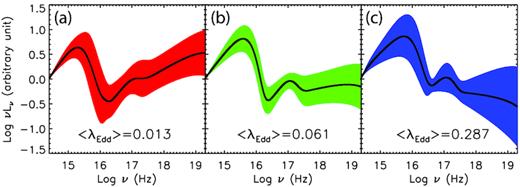
$The averaged SEDs in different Eddington ratio bins, i.e. λEdd ≲ 0.03 (low-, panel (a)), 0.03 ≲ λEdd ≲ 0.09 (intermediate-, panel (b)), and λEdd≳ 0.09 (high-, panel (c)). The black solid line represents the averaged SED, and the coloured regions denote the $68{{\ \rm per\ cent}}$ scatter. The average values of λEdd in each bin are also shown in the panel.$

Figure 9.

The averaged SEDs in different Eddington ratio bins, i.e. λ_Edd ≲ 0.03 (low-, panel (a)), 0.03 ≲ λ_Edd ≲ 0.09 (intermediate-, panel (b)), and λ_Edd≳ 0.09 (high-, panel (c)). The black solid line represents the averaged SED, and the coloured regions denote the |$68{{\ \rm per\ cent}}$| scatter. The average values of λ_Edd in each bin are also shown in the panel.

5.3 Bolometric corrections

The bolometric luminosities obtained above are used to derive bolometric correction factors at a specific luminosity or band,

\begin{eqnarray*} \kappa _{\nu }=\frac{L_{\rm bol}}{\nu L_{\nu }} \end{eqnarray*}

(8)

Here, we focus on two frequently used factors, κ₂₋₁₀ for the 2–10 keV X-ray band and κ₅₁₀₀ at the optical 5100 Å wavelength, respectively.

5.3.1 2–10 keV bolometric correction

The 2–10 keV bolometric correction reflects the relative contribution of the corona X-ray emission in the total radiation power of AGN. Previous studies suggested dependences of κ₂₋₁₀ on a few parameters including |$\rm \lambda _{Edd}$|⁠, Γ_X, and α_OX. Vasudevan & Fabian (2007) found that κ₂₋₁₀ increases with λ_Edd, which was confirmed later in various studies (e.g. Lusso et al. 2010; Jin et al. 2012; Fanali et al. 2013). The distribution of the derived κ₂₋₁₀ for our sample AGN is shown in Fig. 10, spanning a wide range ∼10–100 with a median of ∼19. There is a correlation between κ₂₋₁₀ and λ_Edd (ρ_s = 0.74 and P = 6.4 × 10⁻⁵), consistent with those found in previous studies. The κ₂₋₁₀ versus λ_Edd is plotted in Fig. 11. A bisector regression analysis using the ordinary least-squares algorithm yields a linear relationship equation (9), which is overplotted in Fig. 11.

\begin{eqnarray*} \log \kappa _{2-10}=(0.473\pm 0.068)\log \lambda _{\rm Edd}+(1.922\pm 0.105) \end{eqnarray*}

(9)

The averaged bolometric correction factors are also obtained for the above groups of the Eddington ratios (low-, λ_Edd ≲ 0.03; intermediate-, 0.03 ≲ λ_Edd ≲ 0.09; and high-, λ_Edd ≳ 0.09). κ₂₋₁₀ is found to be 8–15 for λ_Edd ≲ 0.03, 15–30 for 0.03 ≲ λ_Edd ≲ 0.09, and 20–70 for λ_Edd ≳ 0.09. As in previous work, the SSD model was adopted in fitting the optical/UV spectra of AGN, it is of interest to compare our result with previous ones. In Fig. 11, the results from Vasudevan & Fabian (2009) and Fanali et al. (2013) are overplotted for comparison. It can be seen that objects with low- and intermediate- λ_Edd in our sample have similar κ₂₋₁₀ values to those in Vasudevan & Fabian (2009), while the high-λ_Edd objects have lower κ₂₋₁₀ values in general. The slope of the linear regression is flatter (∼3.6σ) than that in Fanali et al. (2013) and predicts lower κ₂₋₁₀ at higher λ_Edd end. This is mainly due to the flatter radial temperature profiles in high-λ_Edd objects than those with low- and intermediate-λ_Edd (see Section 6.4 for a detailed discussion).

Figure 10.

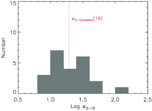
The distribution of the hard X-ray bolometric correction factor κ_2 − 10. The red dotted line represents κ_2 − 10 = 19 (the median).

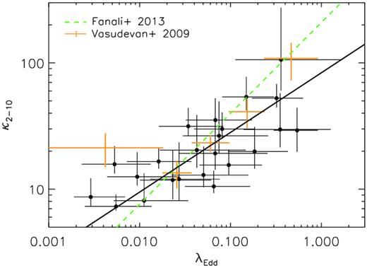
Hard X-ray bolometric correction factor κ2−10 versus Eddington ratio λEdd. The black dots represent the sources in our sample, and the errors are given in 1σ. The black solid line is the bisector regression line. The green dashed line is the best-fitting regression line obtained in Fanali et al. (2013). The yellow crosses are the binned data points in Vasudevan & Fabian (2009).

Figure 11.

Hard X-ray bolometric correction factor κ₂₋₁₀ versus Eddington ratio λ_Edd. The black dots represent the sources in our sample, and the errors are given in 1σ. The black solid line is the bisector regression line. The green dashed line is the best-fitting regression line obtained in Fanali et al. (2013). The yellow crosses are the binned data points in Vasudevan & Fabian (2009).

A relationship between the hard X-ray photon index Γ_X and κ₂₋₁₀ was also found in previous work (e.g. Jin et al. 2012). The distribution of κ₂₋₁₀ versus Γ_X for our sample is plotted in Fig. 12. Only a marginal correlation is found (ρ_s = 0.59 and P = 3.3 × 10⁻³). Using a bisector regression analysis gives

\begin{eqnarray*} \log \kappa _{2-10}=(0.932\pm 0.151)\Gamma _{\rm X}-(0.417\pm 0.278) \end{eqnarray*}

(10)

As suggested by Lusso et al. (2010), α_OX is also an indicator of κ₂₋₁₀, as described by a second-order polynomial relation, and this was later confirmed by Marchese et al. (2012) and Jin et al. (2012). We apply a second-degree polynomial fit to the results in our sample and find

\begin{eqnarray*} \rm \log \kappa _{2-10}=3.97-6.60\alpha _{OX}+3.52\alpha _{OX}^2 \end{eqnarray*}

(11)

The κ₂₋₁₀ versus |$\rm \alpha _{OX}$| distribution is plotted in Fig. 13, along with the relations reported in previous studies. Our fitted curve generally agrees with those derived in Lusso et al. (2010) and Marchese et al. (2012), but lower than that in Jin et al. (2012). Our result confirms that, compared to λ_Edd and Γ_X, α_OX appears to be a better indicator for κ₂₋₁₀. We note that the above correlations (κ_2 − 10-λ_Edd, κ_2 − 10-Γ_X, and κ_2 − 10-α_OX) can also be inferred from the study of the averaged SED (see Fig. 9).

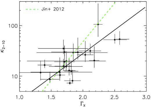
$Hard X-ray bolometric correction factor κ2−10 versus hard X-ray photon index ΓX. The black dots represent the sources in our sample. The error of ΓX is given in $90{{\ \rm per\ cent}}$ confidence interval, and the error of κ2−10 is given in 1σ. The black solid line represents the best-fitting regression. The green dashed line is the result in Jin et al. (2012).$

Figure 12.

Hard X-ray bolometric correction factor κ₂₋₁₀ versus hard X-ray photon index Γ_X. The black dots represent the sources in our sample. The error of Γ_X is given in |$90{{\ \rm per\ cent}}$| confidence interval, and the error of κ₂₋₁₀ is given in 1σ. The black solid line represents the best-fitting regression. The green dashed line is the result in Jin et al. (2012).

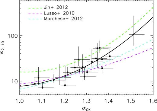
Hard X-ray bolometric correction factor κ2−10 versus effective optical-to-X-ray spectral index αOX. The black dots represent the sources in our sample. The errors are given in 1σ. The black solid line represents the best-fitting polynomial. The pink, green, and cyan dashed lines represent the results reported in Lusso et al. (2010), Jin et al. (2012), and Marchese et al. (2012), respectively.

Figure 13.

Hard X-ray bolometric correction factor κ₂₋₁₀ versus effective optical-to-X-ray spectral index α_OX. The black dots represent the sources in our sample. The errors are given in 1σ. The black solid line represents the best-fitting polynomial. The pink, green, and cyan dashed lines represent the results reported in Lusso et al. (2010), Jin et al. (2012), and Marchese et al. (2012), respectively.

5.3.2 Optical 5100 Å bolometric correction

Early studies suggested a constant 5100 Å bolometric correction factor, e.g. κ₅₁₀₀ = 9.0 (Kaspi et al. 2000) and κ₅₁₀₀ = 10.3 ± 2.1 (Richards et al. 2006), with weak or no dependence of κ₅₁₀₀ on λ_Edd. Vasudevan & Fabian (2007) suggested a positive correlation similar to κ₂₋₁₀, which was confirmed by Jin et al. (2012) using a high-λ_Edd AGN sample. The distribution of κ₅₁₀₀ in our work is shown in Fig. 14, within a range of 8–20 for most of the AGN. The median value of 12 is broadly consistent with 10.3 ± 2.1 given by Richards et al. (2006) for quasars. However, no correlation is found between κ₅₁₀₀ and λ_Edd for our sample (ρ_s = −0.031 and P = 0.89, see Fig. 15), which is in contrary to the results in Vasudevan & Fabian (2007) and Jin et al. (2012). Similar to the case in κ₂₋₁₀, this is also due to the flatter radial temperature profiles in high-λ_Edd objects than those with low- and intermediate-λ_Edd (see Section 6.4 for a detailed discussion).

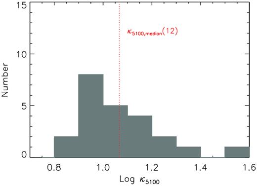
The distribution of the optical (5100 Å) bolometric correction factor κ5100. The red dotted line represents κ5100 = 12 (the median).

Figure 14.

The distribution of the optical (5100 Å) bolometric correction factor κ₅₁₀₀. The red dotted line represents κ₅₁₀₀ = 12 (the median).

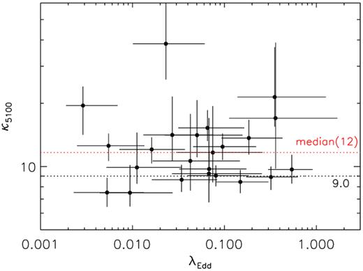
Optical (5100 Å) bolometric correction factor κ5100 versus Eddington ratio λEdd. The black dots represent the sources in our sample. The errors are given in 1σ. The red dotted line represents κ5100 = 12 (the median). The black dotted line represents κ5100 = 9.0 (Kaspi et al. 2000).

Figure 15.

Optical (5100 Å) bolometric correction factor κ₅₁₀₀ versus Eddington ratio λ_Edd. The black dots represent the sources in our sample. The errors are given in 1σ. The red dotted line represents κ₅₁₀₀ = 12 (the median). The black dotted line represents κ₅₁₀₀ = 9.0 (Kaspi et al. 2000).

6 DISCUSSION

6.1 Optical/UV spectral slope

The optical/UV spectrum is of great importance to the determination of the broad-band SED of AGN. The power-law spectral slopes α_opt-UV have been measured for many AGN in large samples in numerous studies using photometric and spectroscopic data from various surveys, e.g. SDSS (Vanden Berk et al. 2001; Davis et al. 2007), Far Ultraviolet Spectroscopic Explorer (FUSE, Scott et al. 2004), Cosmic Origins Spectrograph onboard Hubble Space Telescope (HST/COS, Shull et al. 2012; Stevans et al. 2014), AKARI Space Telescope (Jun et al. 2015), X-shooter onboard Very Large Telescope (VLT/X-shooter, Selsing et al. 2016), and UVOT (Lawther et al. 2017). Despite large scatter, the optical/UV spectra are found to have shallower slopes in most of the studies. The spectral slopes obtained in our work, with elimination of the effects of the host galaxy contamination and dust extinction, are broadly consistent with previous results. Yet, there may be uncertainties inherent in these measurements which may bias the results, as discussed below.

The contamination of the host galaxy starlight is the main source of uncertainty in measuring AGN optical emission at long wavelengths. Bentz et al. (2006) pointed out that even for an aperture of 1 arcsec for AGN photometry the host galaxy contamination may not be negligible. We try to separate the AGN (nuclear) flux from that of the host galaxy by using the 2D image decomposition algorithm galfit, as commonly done in previous work (e.g. Bentz et al. 2009; Vasudevan et al. 2009; Koss et al. 2011), even though the spatial resolution of the UVOT images is not high (a typical FWHM of ∼2 arcsec). To check the reliability of our image decomposition analysis, we compare our results with the previous ones for the seven objects which were also studied for image decomposition by Koss et al. (2011) using the SDSS images with a better resolution. The magnitudes of the galactic component derived in this work are broadly consistent with those derived in Koss et al. (2011) with differences in the fluxes around 10–|$20{{\ \rm per\ cent}}$|⁠. We consider the uncertainties to be small and our results to be reliable.

As commonly adopted in AGN studies, we assume that the dust extinction of the optical/UV continuum can well be represented by that in the broad-line region, which can be estimated from the broad-line Balmer decrement. There is good observational basis for this argument (e.g. Dong et al. 2008; Gaskell 2017). Our sample is selected in such a way that the dust extinction effect is negligible or minor at most. For most (17/23) of our sample objects, the Balmer decrements are consistent with the value for which little or no dust extinction is present. For the remaining six sources, there may be a minor effect and the amount of dust reddening is derived by assuming an SMC-like extinction curve in the analysis. The effect of using different extinction curves is also investigated, including the extinction curves of the MW, the average curves of the Large Magellanic Cloud (LMC) and the LMC2 supershell (Gordon et al. 2003). For these objects, the optical/UV photometric data are corrected for the reddening effect by assuming the above curves. The resulting spectra are fitted with a power-law model as well as the p-free disc model, respectively. This results in typical changes in the optical/UV slopes of ∼5 per cent only and ∼2 per cent in the index p. We thus conclude that the use of different extinction curves does not affect our results significantly for those objects in which minor dust reddening might occur. Therefore, in the rest of this work, the SMC-like extinction curve is adopted.

6.2 Accretion discs with non-standard radial temperature profile

It has been demonstrated that the shallower spectral slopes in our sample AGN cannot be attributed mainly to starlight contamination or dust reddening. We consider such spectral shapes intrinsic to the emission from the AGN, which can well be produced by an accretion disc with a radial temperature profile flatter than the canonical T_eff(R) ∝ R^−0.75 for the standard SSD model. Theoretically, the spectral slope α of the power-law regime of an accretion disc spectrum and the effective temperature power-law index p are related via α = 3 − 2/p (e.g. Pringle & Rees 1972; Kato et al. 2008). For SMBHs, the power-law regime of the spectra falls into the optical/UV waveband for a wide range of M_BH and λ_Edd, and the slope α_opt-UV can be reddened depending on the exact value of p. Gaskell (2008) suggested that p ≈ −0.57 can explain the typical spectral slopes of α ≈ −0.5 observed in AGN. In this work, we apply this model, for the first time, to fit the optical/UV spectra for a sample of AGN with simultaneous multi-band photometric data. It is found that, the inferred radial effective temperature profile indices p fall within a range of 0.5–0.75 for most of the sample objects in order to explain the observed spectra, flatter than p = 0.75 for the SSD widely assumed in previous studies.

Accretion discs with a non-standard radial temperature profile (p ≠ 0.75) may operate if one or more of the assumptions underlying the standard SSD break down. For instance, the local thermal equilibrium condition may not hold, if the dissipated accretion energy cannot be radiated away efficiently locally, and consequently the energy/photons are advected into the black hole. Alternatively, the assumption of mass conservation may not hold as, for instance, part of the accreted mass is lost in the accretion process due to various mechanisms (e.g. disc winds/outflows).

To gain an insight into the cause of the non-standard radial temperature profiles, the relationship is examined between p and the Eddington ratio λ_Edd, which is considered to be the most possible dominant quantity that governs the accretion process of AGN. A marginal correlation is found (ρ_s = −0.41, and P = 5.0 × 10⁻²), as shown in Fig. 16, where the results derived using different dust extinction curves for the sources with intrinsic reddening are marked in different colours. The correlation becomes more prominent when only the sources having no intrinsic dust reddening are used (ρ_s = −0.71, and P = 1.4 × 10⁻³). Such a correlation is qualitatively consistent with the above physical explanations. For instance, when the accretion rate is well below the Eddington limit, the radiative diffusion time-scale in the disc is much faster than the accretion time-scale. Such an accretion flow is radiatively efficient and has a radial temperature distribution of SSD type (T_eff(R) ∝ R^−0.75). However, when the accretion rate approaches the Eddington limit (λ_Edd ≳ 0.3, e.g. Abramowicz et al. 1988; Mineshige et al. 2000), the photon trapping effect in the disc becomes appreciable and the disc becomes a ‘slim’ disc. In this case, the radiation energy is trapped and advected inward rather than locally radiated away, resulting in a much flatter radial temperature profile (T_eff(R) ∝ R^−0.5, e.g. Wang et al. 1999; Watarai & Fukue 1999). Given the distribution of the Eddington ratio of our sample, the flat temperature profiles in most of the sources can hardly be induced by the photon trapping. Nevertheless, we suggest that this effect may operate in some of the high-λ_Edd sources and be partly responsible for the observed p–λ_Edd correlation.

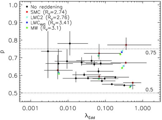
$Power-law index of the radial temperature profile p versus Eddington ratio λEdd. Black dots are the sources with ${\rm H{\alpha }/{\rm H{\beta }}}\le 3.06$. Coloured dots are the sources with ${\rm H{\alpha }/{\rm H{\beta }}}\gt 3.06$ dereddened using various extinction curves (red: SMC, cyan: LMC2, blue: average LMC, and green: MW). The two black dotted lines represent p = 0.75 (SSD solution) and p = 0.5 (‘slim’ disc solution). The errors are given in 1σ.$

Figure 16.

Power-law index of the radial temperature profile p versus Eddington ratio λ_Edd. Black dots are the sources with |${\rm H{\alpha }/{\rm H{\beta }}}\le 3.06$|⁠. Coloured dots are the sources with |${\rm H{\alpha }/{\rm H{\beta }}}\gt 3.06$| dereddened using various extinction curves (red: SMC, cyan: LMC2, blue: average LMC, and green: MW). The two black dotted lines represent p = 0.75 (SSD solution) and p = 0.5 (‘slim’ disc solution). The errors are given in 1σ.

Another possible physical explanation is offered by the mass-loss process in form of outflows/disc winds, as a power-law radial temperature profile with an index p ≠ 0.75 implies a non-stationary mass inflow rate |$\dot{M}(R)\propto R^{3-4p}$| under the LTE assumption. In fact, observations suggest that outflows may be prevalent or even ubiquitous in bright AGN, and are likely stronger in higher-λ_Edd objects (e.g. Laor & Brandt 2002; Ganguly et al. 2007; Zhang et al. 2014). In this picture, the p–λ_Edd relation found in our work can thus be understood, as the p-value is determined by the amount of mass loss, i.e. a smaller p-value (a steeper mass flow rate distribution and thus a stronger mass loss) tends to be found in higher-λ_Edd objects. Interestingly, Gofford et al. (2015) studied the properties of highly ionized outflows for a sample of 51 AGN observed with Suzaku and found that the mass-loss rate of the outflow (⁠|${\dot{M}}_{\rm loss}$|⁠) is well correlated with the bolometric luminosity (L_bol) of the source. Recently, it has been well interpreted under the mechanism of the line-driven disc wind by numerical simulations (e.g. Nomura & Ohsuga 2017; Nomura, Ohsuga & Done 2018). In this work, by assuming that the deviation of the radial temperature profile is caused by the mass-loss process, we can also investigate the |${\dot{M}}_{\rm loss}$|–L_bol relation from the spectral fitting results.

In order to calculate the mass-loss rate for the sample AGN, the mass flow rate profile |$\dot{M}(R)$| for each object is obtained from the best-fitting radial temperature distribution T_eff(R) (see Section 4.2) under the LTE assumption (⁠|$T_{\rm eff}(R)=f(\dot{M}(R), M_{\rm BH},R)\propto \dot{M}(R)^{1/4}M_{\rm BH}^{1/4}R^{-3/4}$|⁠, e.g. Frank et al. 2002; Kato et al. 2008). With this accretion rate profile, the mass-loss rate is calculated by

\begin{eqnarray*} \dot{M}_{\rm loss}=\dot{M}(R_{\rm out})-\dot{M}(R_{\rm in}) \end{eqnarray*}

(12)

We note that the mass-loss rate is positive when p < 0.75 and negative when p > 0.75. For the latter case, this indicates an ‘inflow’ instead of ‘outflow’. In this work, we do not take this ‘inflow’ explanation for the sources with |$p\gtrsim 0.75$|⁠, considering the uncertainties inherent in our spectral fitting procedure. The accretion discs in these sources are regarded to be the SSD-type. We also note that although the mass-loss rate formally depends both on p and T_eff(R_in), the dependence on p is decisive as it appears in the power-law index of the accretion rate formula thus determines the steepness of the distribution. In other words, no matter how large T_eff(R_in) (the accretion rate at R_in) is, a p-value close to 0.75 (the SSD solution) stands for a weak/negligible outflow solution (⁠|$\dot{M}_{\rm loss}\approx 0$|⁠).

The bolometric luminosity L_bol is derived by integrating the SED model within the energy range of 0.001–300 keV. We note that L_bol depends mainly on T_eff(R_in), and the relation can roughly be a fourth power when L_bol ≈ L_disc under high-λ_Edd condition. The dependence on p, however, is inconspicuous (there is no statistical correlation between L_bol and p). One should keep in mind that the two free parameters p and T_eff(R_in) is not correlated (the former is determined by the optical/UV spectral slope, and the latter by the observed flux). Fig. 17 shows the obtained relation between |${\dot{M}}_{\rm loss}$| (in units of |$\rm g\ s^{-1}$|⁠) and the bolometric luminosity L_bol for 17 sources with p < 0.75 in our sample (in other six sources, the stationary disc solution p = 0.75 can be satisfied considering the uncertainties). It is clear that the resulting relation is in agreement with the observational result obtained by Gofford et al. (2015). Since the mass-loss rate and bolometric luminosity derived in our work can be regarded as irrelevant to each other, as we showed above, the relation obtained here is an independent proof that verifies the results in their work. This also suggests that the observed reddened optical/UV spectra in the AGN of our sample are likely a result of the flatter radial temperature profiles of their accretion discs than the standard SSD profile. Such a flat temperature profile may be caused by mass loss in the form of outflows as the mass is accreted inward.

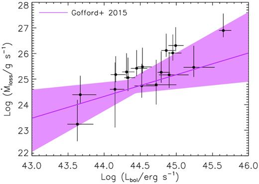
$Mass-loss rate within the disc $\dot{M}_{\rm loss}$ versus bolometric luminosity Lbol. The black crosses are the sample objects (excluding six sources in which the SSD solution can be satisfied, see the text). The errors are given in 1σ. The pink solid line and shallow region represent the best-fitting regression relation and 1σ error derived in Gofford et al. (2015).$

Figure 17.

Mass-loss rate within the disc |$\dot{M}_{\rm loss}$| versus bolometric luminosity L_bol. The black crosses are the sample objects (excluding six sources in which the SSD solution can be satisfied, see the text). The errors are given in 1σ. The pink solid line and shallow region represent the best-fitting regression relation and 1σ error derived in Gofford et al. (2015).

Apart from these two scenarios, the deviation of the radial temperature profile could also result from an accretion disc illuminated by an external radiation source (e.g. Czerny et al. 2008), or the irradiation of the outer areas by its inner part (e.g. Sanbuichi et al. 1993). By introducing an additional heating term which is more pronounced in the outer areas of the AGN disc, a flattened radial temperature profile can be obtained and lead to a reddened optical/UV spectra (e.g. Soria & Puchnarewicz 2002; Loska et al. 2004). However, this usually requires the disc to be warped (H_d ≈ R, H_d is the vertical height of the disc at radius R, e.g. Pringle 1997). In our work, we only consider flat (geometrically thin) accretion discs (H_d ≪ R). In this case, the irradiating disc gives a radial dependence of the temperature identical to the one derived for the SSD (see Netzer 2013, chapter 4.2.2).

6.3 Implication to the SED modelling of AGN

In the modelling of the AGN optical/UV continuum in previous studies, the spectrum from the SSD model is mostly adopted and assumed to be subject to dust reddening with E(B − V) as a free-fitting parameter (e.g. Vasudevan & Fabian 2009; Vasudevan et al. 2009; Capellupo et al. 2016; Castelló-Mor, Netzer & Kaspi 2016). While such a model can reproduce the observed optical/UV spectra reasonably well, it implies an enormous energy budget of the intrinsic source luminosity in the far- and extreme-UV regime, where the multitemperature blackbody from the accretion disc peaks (the so-called ‘BBB’). On the other hand, the p-free disc model with a flat radial temperature profile leads to a less prominent EUV bump and a lower peak energy (due to lower T_eff in the inner disc), and thus lower energy output. Given that the bolometric luminosity is dominated by the energy in this regime, the two models may result in somewhat different bolometric luminosities. In another word, if in reality, the accretion disc is indeed better described by a non-standard radial temperature profile, the bolometric luminosities calculated assuming the SSD model must be overestimated systematically to some extent.

As a demonstration, a quantitive comparison between the broad-band SED based on the two models is carried out for two selected objects in our sample with shallower spectral slopes, SBS 1136 + 594 (α_opt-UV = −0.2) and Mrk 493 (α_opt-UV = −0.12). Their optical/UV spectra can be fitted equally well with the SSD model which is reddened using the SMC extinction curve with E(B − V) as a free parameter. The fitted broad-band SED model is plotted in Fig. 18, together with those obtained assuming the p-free disc model above in this work. An excess dust reddening of E(B − V) (0.08 and 0.12, respectively) is required to reproduce the observed optical/UV spectra in both sources, albeit their Balmer decrements (<3.06) indicate no reddening. The overall disc luminosities based on the SSD model is higher than that for the p-free disc model by a factor of 3.4 and 5.9, respectively. The differences are comparable to those derived in Slone & Netzer (2012), in which the accretion energy carried away by disc winds is considered in calculating the emergent radiation of the accretion disc, effectively similar to the approach adopted in this work. This results in an overestimation of the bolometric luminosity L_bol by a factor of 2.1 and 5.0, respectively. The difference would be even more pronounced for sources with even more flatter radial temperature profiles (for instance, for RX J1702.5 + 3247 in which p ≈ 0.54 the difference in L_bol is around 8.0).

Figure 18.

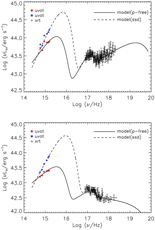
Two examples (upper panel: SBS 1136 + 594, and lower panel: Mrk 493) showing the difference in the intrinsic luminosities in optical/UV bands and the broad-band SEDs when using two methods in optical/UV spectral fitting, i.e. the p-free disc model employed in this work and the SSD model with the intrinsic dust reddening E(B − V) set as a free parameter. The intrinsic luminosities in the six UVOT filters obtained by the above two methods are marked with red dots and blue dots. The two broad-band SED models derived by two methods are represented by the solid and dashed lines, respectively.

http://www.asdc.asi.it/mmia/index.php?mission = swiftmastr

We note that the uncertainties inherent in our method should be considered when assessing the significance of this difference. In this work, we implement the estimation of the uncertainties in two ways. For the optical/UV band, we employ the Monte Carlo method to estimate the uncertainty in L_disc, which is caused by the systematics of various physical parameters in the p-free disc model (M_BH, i, a_*). As for the X-ray (corona) luminosity, the statistical error is calculated using xspec/cflux. By the combination of these two methods, the 1σ uncertainty in L_bol is found to be 0.1–0.3 dex for the sample objects (see Table 6). In this sense, the differences in L_bol obtained in a moderate fraction of the sample (8/23) are somewhat significant as they exceed the uncertainties (the differences are by a factor of 4–8). However, we should keep in mind that there are certainly other contributions to the uncertainty in L_bol which are not considered in this estimation. For instance, the contribution of the soft excess below the lower end of the Swift/XRT bandpass is difficult to be robustly constrained by the blackbody model. In fact, there are various physical models in describing this mystical component, such as the thermal comptonization model (e.g. Magdziarz et al. 1998; Done et al. 2012) and the blurred ionized reflection model (e.g. Crummy et al. 2006). As a pilot test, we attempt the thermal comptonization model optxagnf (Done et al. 2012) to some of the sample AGN in which a strong soft X-ray excess exists (e.g. Mrk 142, RX J1355.2+5612, RX J1702.5 + 3247) and find that the derived bolometric luminosities are higher than those derived in this work by a factor of 3–4. This indicates that alternative models of the soft excess may also lead to an overestimation of L_bol. As a first study of the effects caused by using the p-free disc model, we mainly pay our attention to the distinction in the optical/UV band. Further investigations including a more physical model in describing the soft excess will be implemented in future work.

Our results show that the traditional way in modelling the optical/UV spectra (the SSD model subject to an additional dust reddening) could indeed lead to an overestimation of the disc luminosity when the intrinsic spectra are found to be redder than that of the SSD. As the redder-than-SSD spectra have been widely observed in the literature and the disc luminosity usually dominates the overall energy budget, this also suggests that the bolometric luminosities and hence the Eddington ratios for many AGN may have been overestimated in some of the previous studies (probably by a factor of several).

6.4 Bolometric correction factors

The bolometric correction factor κ_ν is a convenient quantity used to derive the bolometric luminosity L_bol (representing the accretion rate |$\dot{M}$|⁠) of an AGN based on photometric measurement in a specific waveband. The commonly used factors are κ₂₋₁₀ for the X-ray band and κ₅₁₀₀ for the optical. There have been studies on κ₅₁₀₀ and κ₂₋₁₀ in the literature, which are found to be dependent on some other parameters in some of the studies. For instance, a strong correlation between κ₂₋₁₀ and λ_Edd was reported (e.g. Vasudevan & Fabian 2007, 2009; Vasudevan et al. 2009; Lusso et al. 2010). The hard X-ray photon index Γ_X (e.g. Jin et al. 2012) and the optical-to-X-ray effective index α_OX (e.g. Lusso et al. 2010; Marchese et al. 2012) were also suggested to correlate with κ₂₋₁₀. As for the optical band, a correlation between κ₅₁₀₀ and λ_Edd was reported in Vasudevan & Fabian (2007) and later confirmed by Jin et al. (2012). These correlations were mostly derived from the broad-band SED analysis assuming the SSD model in the optical/UV and EUV bands. As discussed above, for those sources with reddened optical/UV spectra the employment of the p-free disc model implies a much lower EUV bump and hence a smaller L_bol compared to the SSD model. It is therefore of interest to re-investigate the bolometric correction factors and their dependence on some of the key parameters.

Compared to Vasudevan et al. (2009), the increase of κ₂₋₁₀ with λ_Edd is found to be less steep in our work (see Section 5.3.1). This is because a large fraction of the high-λ_Edd sources (λ_Edd ≳ 0.1) have a relatively lowered κ₂₋₁₀ values compared to Vasudevan et al. (2009), while the κ₂₋₁₀ values are similar for the objects with low- and intermediate- λ_Edd (see Fig. 11). Since the spectral modelling in the X-ray band is not affected by that in the optical/UV band, the decrease in L_disc by using the p-free disc model leads to a decrease in L_bol, and hence κ₂₋₁₀ and λ_Edd which are both proportional to L_bol. This effect, although present in nearly all AGN of our sample, affects mostly the high-λ_Edd sources since they have much flatter radial temperature profiles (smaller p values) than the low- and intermediate-λ_Edd objects (see Fig. 16). Compared to the results obtained based on the SSD model, this results in a lower κ₂₋₁₀ for the same λ_Edd at the higher λ_Edd end and thus flatten the κ_2−10–λ_Edd relation.

The optical correction factor κ₅₁₀₀ is found to be independent of λ_Edd in our work, which differs from previous studies (e.g. Vasudevan & Fabian 2007; Jin et al. 2012). The correlations reported in those studies were mainly due to an increase of κ₅₁₀₀ at the higher λ_Edd end (there is little or no correlation among low- and intermediate-λ_Edd objects). In our case, however, this trend is weakened since the high-λ_Edd objects have significantly lowered κ₅₁₀₀ (while the values of κ₅₁₀₀ in low- and intermediate-λ_Edd objects are similar). Unlike κ₂₋₁₀, the effect on κ₅₁₀₀ by using different disc models is more complex since both L₅₁₀₀ and L_bol are inherent to the model and changed (see Fig. 18). To understand the difference in the high-λ_Edd regime between the two models, we calculate the theoretical κ₅₁₀₀ values for the same range of black hole mass M_BH (10⁷–10⁸|$\, \mathrm{M}_{\odot }$|⁠) and Eddington ratio λ_Edd (0.1–1.0) in the framework of the SSD model (the fraction of corona emission in the total luminosity is assumed to be |$5{{\ \rm per\ cent}}$|⁠, as estimated from the hard X-ray bolometric correction for high-λ_Edd sources in Vasudevan & Fabian 2009). The theoretical values of κ₅₁₀₀ lie between 30–80, which are much larger than the values derived based on the p-free disc model in our work (9–20). This is caused by the enormous difference in the radiative energy in the EUV band from the inner disc region (L ∝ T_eff(R_in)⁴), where the two models have very different temperatures. We note that the median value of κ₅₁₀₀ ≈12 obtained in our work is generally consistent with those given in some of the previous studies (e.g. Richards et al. 2006).

7 SUMMARY

We present a study on the broad-band SED for a well-selected sample of Seyfert 1 galaxies, by taking advantage of their simultaneous optical, UV, and X-ray observations with the Neil Gehrels Swift Observatory. Their SDSS spectrometric data are also used to derive the optical spectral parameters in order to determine their BH masses and Balmer decrements. The sample is selected in a way that there is little or no intrinsic dust reddening as indicated by the Balmer decrement of the broad emission lines. The starlight contamination of the host galaxies is eliminated to a large extent by performing 2D nuclear-galaxy image decomposition.

The main feature of this work that differs from previous studies is that we employ, for the first time, an accretion disc model with a generalized radial temperature profile (rather than the standard SSD profile with the emergent spectra modified by dust reddening) to fit the observed optical/UV spectra of AGN. That is, the power-law index of the radial temperature distribution is treated as a free parameter (T_eff(R) ∝ R^−p, i.e. the p-free disc model), which is a special case when p = 0.75 as commonly adopted in previous studies. The underlying physics of such a model concerns possible breakdown in reality of the assumptions on which the SSD model is based, e.g. the mass conservation of the inward accretion flow or the effective radiative cooling of the disc.

It is found that the majority of our sample AGN show a shallower optical/UV spectral slope (F_ν ∝ ν^α, α = −1.0 to +0.3 with a median of −0.39) after correcting for host galaxy starlight and dust reddening wherever applicable. This is broadly consistent with previous results and at odds with the prediction by the SSD solution (α = +1/3), implying in general flatter radial temperature profiles than the latter. By fitting the p-free disc model to the optical/UV spectra, the radial temperature power-law indices are derived, p = 0.5–0.75 (median 0.63), smaller than the SSD value p = 0.75 for most of our sample objects. We suggest that the reddened optical/UV spectra as observed in many AGN are at least in part determined by the intrinsically reddened spectral shape of the disc emission.

The broad-band SED of our sample AGN are constructed by integrating the p-free disc model in the optical/UV band and the X-ray radiation model derived from the simultaneous X-ray observations. The averaged SEDs are also presented, whose shapes are found to be dependent strongly on the Eddington ratio. The bolometric luminosities and the bolometric correction factors in the optical κ₅₁₀₀ and X-ray band κ₂₋₁₀ are derived. It is found that, for sources with reddened optical/UV spectra typical of AGN, the SSD plus dust reddening model as commonly adopted in previous work can lead to disc luminosities higher than those derived from the p-free disc model by a factor of several, as well as the bolometric luminosities. The difference is more pronounced in AGN with higher Eddington ratios. Consequently, the values of κ₂₋₁₀ and κ₅₁₀₀ as well as their relations with λ_Edd are affected. The hard X-ray bolometric correction factor κ₂₋₁₀ is found to be 8–15 for λ_Edd ≲ 0.03 and 15–30 for 0.03 ≲ λ_Edd ≲ 0.09, which is similar to previous results. κ₂₋₁₀ at high λ_Edd values (λ_Edd ≳ 0.1) are relatively lower (20–70) than previous results. The optical bolometric correction factor κ₅₁₀₀ is found to be independent of the Eddington ratio λ_Edd, with a median value of ∼12.

The physical origin of the flattened temperature profile in an accretion disc is complicated and far from fully understood. In this work, we suggest that some kind of mass-loss process in form of disc winds/outflows could be a possible scenario for this issue. A thorough test of this hypothesis will be needed in future work.

ACKNOWLEDGEMENTS

We thank the anonymous referee for very helpful suggestions. This work is supported by the National Natural Science Foundation of China (grant nos 11473035, 11673026, 11873054, 11803047, and 11773037) and the Strategic Pioneer Program on Space Science, Chinese Academy of Sciences (grant no. XDA15052100). AAB is supported by UK Space Agency. CJ is supported by the Hundred Talents Program of the Chinese Academy of Sciences. We are very grateful to S. Komossa, R. Taam, Xiaobo Dong, and Hongyan Zhou for useful comments and suggestions. HQ thanks R. Vasudevan for precious comments in UVOT data procedure, and Zhu Liu for help in X-ray data analysis. This work is mainly based on observations obtained by the Neil Gehrels Swift Observatory. We acknowledge the entire Swift team for providing the data that made this work possible. We have also made use of the data products from the SDSS. This research has made use of the NASA/IPAC Extra-galactic Database (NED).

Footnotes

1

We note that the emission in the mid- and far-infrared (IR) waveband is not included in this study, as it is known to be re-processed from the UV emission by torus (e.g. Antonucci 1993; Netzer 2015).

2

3

https://dr13.sdss.org/home

4

http://www.swift.ac.uk/analysis/uvot/index.php

5

We find that for a few cases the PSF flux after the coincidence correction exceeds that obtained by uvotsource using the standard 5 arcsec aperture. Considering that there is some scope for error in the coincidence loss correction when the PSF image is extended, we simply choose the 5 arcsec aperture photometry.

6

Considering the relatively low redshifts and UVOT coverage (1928, 2246, 2600, 3465, 4392, 5468 Å), Mg II (2798 Å, rest frame) is the main contaminant in uvw1 and u filters. AI III (1958 Å) + C III (1909 Å) might be another contaminant in uvw2 filter. However, for the majority of the sample objects, the emission line contamination was estimated to be a negligible effect in previous studies (Vasudevan et al. 2009; Grupe et al. 2010)

7

http://www.swift.ac.uk/analysis/xrt/index.php

8

http://users.ynao.ac.cn/ xbdong/

9

Generally, R_out ≳ 1000R_s for a black hole with a mass of |$10^8 \, \mathrm{M}_{\odot }$|⁠. Considering that the temperature in lower mass black holes (⁠|$M_{\rm BH}\approx 10^7\, \mathrm{M}_{\odot }$|⁠) is relative higher and the emission from outer radius can have a contribution to the emission in optical band, we take a commonly adopted value 3000R_s.

10

The power-law model drops toward low energies as an exponential decay |$\exp ^{-E_{\rm cut, low}/{E}}$| in EUV band. The E_{cut, low} is determined for each individual source as (1) 4E_{cut, low} ≥ E_scat, where E_scat = 2.4E_{disc, peak} represents the minimum scattered energy after inverse Compton scattering; and (2) the peak of the continuum is determined by the fitted accretion disc model above.

11

We note that the uncertainty of α_OX is dominated by that of L₂₅₀₀ as it has a larger uncertainty than |$L(\rm 2keV)$|⁠.

REFERENCES

Abramowicz

M. A.

,

Czerny

B.

,

Lasota

J. P.

,

Szuszkiewicz

E.

,

1988

,

ApJ

,

332

,

646

10.1086/166683

10.1088/0004-637X/727/1/31

Ai

Y. L.

,

Yuan

W.

,

Zhou

H. Y.

,

Wang

T. G.

,

Zhang

S. H.

,

2011

,

ApJ

,

727

,

31

10.1146/annurev.aa.31.090193.002353

Antonucci

R.

,

1993

,

ARA&A

,

31

,

473

Arnaud

K. A.

,

1996

, in

Jacoby

G. H.

,

Barnes

J.

, eds,

ASP Conf. Ser., Vol. 101, Astronomical Data Analysis Software and Systems V

.

Astron. Soc. Pac

,

San Francisco

, p.

17

10.3847/0004-637X/832/1/8

Baron

D.

,

Stern

J.

,

Poznanski

D.

,

Netzer

H.

,

2016

,

ApJ

,

832

,

8

10.1088/0004-637X/697/1/160

Bentz

M. C.

,

Peterson

B. M.

,

Netzer

H.

,

Pogge

R. W.

,

Vestergaard

M.

,

2009

,

ApJ

,

697

,

160

Bentz

M. C.

,

Peterson

B. M.

,

Pogge

R. W.

,

Vestergaard

M.

,

Onken

C. A.

,

2006

,

ApJ

,

644

,

133

10.1086/503537

10.1111/j.1365-2966.2010.16832.x

Breeveld

A. A.

et al. .,

2010

,

MNRAS

,

406

,

1687

Burrows

D. N.

et al. .,

2005

,

Space Sci. Rev.

,

120

,

165

Capellupo

D. M.

,

Netzer

H.

,

Lira

P.

,

Trakhtenbrot

B.

,

Mejía-Restrepo

J.

,

2016

,

MNRAS

,

460

,

212

10.1093/mnras/stw937

Castelló-Mor

N.

,

Netzer

H.

,

Kaspi

S.

,

2016

,

MNRAS

,

458

,

1839

10.1093/mnras/stw445

10.1111/j.1365-2966.2005.09844.x

Crummy

J.

,

Fabian

A. C.

,

Gallo

L.

,

Ross

R. R.

,

2006

,

MNRAS

,

365

,

1067

Czerny

B.

,

2007

, in

Ho

L. C.

,

Wang

J.-W.

, eds,

ASP Conf. Ser., Vol. 373, The Central Engine of Active Galactic Nuclei

.

Astron. Soc. Pac

,

San Francisco

, p.

586

10.1111/j.1365-2966.2011.18912.x

Czerny

B.

,

Goosmann

R.

,

Janiuk

A.

,

2008

,

Chin. J. Astron. Astrophys. Suppl.

,

8

,

302

Czerny

B.

,

Hryniewicz

K.

,

Nikołajuk

M.

,

Sa̧dowski

A.

,

2011

,

MNRAS

,

415

,

2942

10.1051/0004-6361:20077569

Dadina

M.

,

2008

,

A&A

,

485

,

417

Davis

S. W.

,

El-Abd

S.

,

2019

,

ApJ

,

874

,

23

Davis

S. W.

,

Woo

J.-H.

,

Blaes

O. M.

,

2007

,

ApJ

,

668

,

682

10.1086/521393

10.1111/j.1365-2966.2011.19779.x

Done

C.

,

Davis

S. W.

,

Jin

C.

,

Blaes

O.

,

Ward

M.

,

2012

,

MNRAS

,

420

,

1848

Done

C.

,

Jin

C.

,

2016

,

MNRAS

,

460

,

1716

10.1093/mnras/stw1070

10.1111/j.1365-2966.2007.12560.x

Dong

X.

,

Wang

T.

,

Wang

J.

,

Yuan

W.

,

Zhou

H.

,

Dai

H.

,

Zhang

K.

,

2008

,

MNRAS

,

383

,

581

Dong

X.-B.

,

Zhou

H.-Y.

,

Wang

T.-G.

,

Wang

J.-X.

,

Li

C.

,

Zhou

Y.-Y.

,

2005

,

ApJ

,

620

,

629

10.1086/427174

Elvis

M.

et al. .,

1994

,

ApJS

,

95

,

1

10.1086/192093

Fanali

R.

,

Caccianiga

A.

,

Severgnini

P.

,

Della Ceca

R.

,

Marchese

E.

,

Carrera

F. J.

,

Corral

A.

,

Mateos

S.

,

2013

,

MNRAS

,

433

,

648

10.1093/mnras/stt757

Frank

J.

,

King

A.

,

Raine

D. J.

,

2002

,

Accretion Power in Astrophysics: Third Edition

.

Cambridge Univ. Press

,

Cambridge, UK

, p.

398

Ganguly

R.

,

Brotherton

M. S.

,

Cales

S.

,

Scoggins

B.

,

Shang

Z.

,

Vestergaard

M.

,

2007

,

ApJ

,

665

,

990

10.1086/519759

Gaskell

C. M.

,

2008

,

Rev. Mex. Astron. Astrofis.

,

32

,

1

Gaskell

C. M.

,

2017

,

MNRAS

,

467

,

226

10.1093/mnras/stx094

Gaskell

C. M.

,

Goosmann

R. W.

,

Antonucci

R. R. J.

,

Whysong

D. H.

,

2004

,

ApJ

,

616

,

147

10.1086/423885

Gaskell

C. M.

,

Klimek

E. S.

,

Nazarova

L. S.

,

2007

,

preprint

(arXiv:0711.1025)

Gebhardt

K.

et al. .,

2000

,

ApJ

,

543

,

L5

10.1086/318174

Gehrels

N.

et al. .,

2004

,

ApJ

,

611

,

1005

10.1086/422091

Gofford

J.

,

Reeves

J. N.

,

McLaughlin

D. E.

,

Braito

V.

,

Turner

T. J.

,

Tombesi

F.

,

Cappi

M.

,

2015

,

MNRAS

,

451

,

4169

10.1093/mnras/stv1207

Gordon

K. D.

,

Clayton

G. C.

,

Misselt

K. A.

,

Landolt

A. U.

,

Wolff

M. J.

,

2003

,

ApJ

,

594

,

279

10.1086/376774

Greene

J. E.

,

Ho

L. C.

,

2006

,

ApJ

,

641

,

L21

10.1086/500507

10.1088/0004-637X/773/2/90

Grier

C. J.

et al. .,

2013

,

ApJ

,

773

,

90

10.1088/0067-0049/187/1/64

Grupe

D.

,

Komossa

S.

,

Leighly

K. M.

,

Page

K. L.

,

2010

,

ApJS

,

187

,

64

Hirano

A.

,

Kitamoto

S.

,

Yamada

T. T.

,

Mineshige

S.

,

Fukue

J.

,

1995

,

ApJ

,

446

,

350

10.1086/175793

Hopkins

P. F.

et al. .,

2004

,

AJ

,

128

,

1112

10.1086/423291

Ichimaru

S.

,

1977

,

ApJ

,

214

,

840

10.1086/155314

Jin

C.

,

Done

C.

,

Ward

M.

,

Gardner

E.

,

2017

,

MNRAS

,

471

,

706

10.1093/mnras/stx1634

10.1111/j.1365-2966.2012.21272.x

Jin

C.

,

Ward

M.

,

Done

C.

,

2012

,

MNRAS

,

425

,

907

10.1088/0004-637X/806/1/109

Jun

H. D.

et al. .,

2015

,

ApJ

,

806

,

109

Kaspi

S.

,

Smith

P. S.

,

Netzer

H.

,

Maoz

D.

,

Jannuzi

B. T.

,

Giveon

U.

,

2000

,

ApJ

,

533

,

631

10.1086/308704

Kato

S.

,

Fukue

J.

,

Mineshige

S.

,

2008

,

Black-Hole Accretion Disks — Towards a New Paradigm

,

Kyoto Univ. Press

,

Kyoto, Japan

.

10.1146/annurev-astro-082214-122316

King

A.

,

Pounds

K.

,

2015

,

ARA&A

,

53

,

115

Koratkar

A.

,

Blaes

O.

,

1999

,

PASP

,

111

,

1

10.1086/316294

10.1088/0004-637X/739/2/57

Koss

M.

,

Mushotzky

R.

,

Veilleux

S.

,

Winter

L. M.

,

Baumgartner

W.

,

Tueller

J.

,

Gehrels

N.

,

Valencic

L.

,

2011

,

ApJ

,

739

,

57

10.1088/0004-6256/149/6/203

Krawczyk

C. M.

,

Richards

G. T.

,

Gallagher

S. C.

,

Leighly

K. M.

,

Hewett

P. C.

,

Ross

N. P.

,

Hall

P. B.

,

2015

,

AJ

,

149

,

203

10.1088/0067-0049/206/1/4

Krawczyk

C. M.

,

Richards

G. T.

,

Mehta

S. S.

,

Vogeley

M. S.

,

Gallagher

S. C.

,

Leighly

K. M.

,

Ross

N. P.

,

Schneider

D. P.

,

2013

,

ApJS

,

206

,

4

Kubota

A.

,

Ebisawa

K.

,

Makishima

K.

,

Nakazawa

K.

,

2005

,

ApJ

,

631

,

1062

10.1086/432900

Kubota

A.

,

Makishima

K.

,

2004

,

ApJ

,

601

,

428

10.1086/380433

La Mura

G.

,

Popović

L. Č.

,

Ciroi

S.

,

Rafanelli

P.

,

Ilić

D.

,

2007

,

ApJ

,

671

,

104

10.1086/522821

Laor

A.

,

Brandt

W. N.

,

2002

,

ApJ

,

569

,

641

10.1086/339476

Laor

A.

,

Davis

S. W.

,

2014

,

MNRAS

,

438

,

3024

10.1093/mnras/stt2408

Laor

A.

,

Netzer

H.

,

1989

,

MNRAS

,

238

,

897

10.1093/mnras/238.3.897

Lawther

D.

,

Vestergaard

M.

,

Raimundo

S.

,

Grupe

D.

,

2017

,

MNRAS

,

467

,

4674

10.1093/mnras/stx423

Li

A.

,

2007

, in

Ho

L. C.

,

Wang

J.-W.

, eds,

ASP Conf. Ser. Vol. 373, The Central Engine of Active Galactic Nuclei

.

Astron. Soc. Pac

,

San Francisco

, p.

561

10.1088/0004-637X/707/1/233

Liu

B. F.

,

Taam

R. E.

,

2009

,

ApJ

,

707

,

233

10.1088/0004-637X/806/2/223

Liu

B. F.

,

Taam

R. E.

,

Qiao

E.

,

Yuan

W.

,

2015

,

ApJ

,

806

,

223

Liu

H.-Y.

,

Yuan

W.

,

Dong

X.-B.

,

Zhou

H.

,

Liu

W.-J.

,

2018

,

ApJS

,

235

,

40

10.3847/1538-4365/aab88e

10.3847/0004-637X/822/2/64

Liu

W.-J.

et al. .,

2016

,

ApJ

,

822

,

64

10.1111/j.1365-2966.2004.08387.x

Loska

Z.

,

Czerny

B.

,

Szczerba

R.

,

2004

,

MNRAS

,

355

,

1080

10.1051/0004-6361/200913298

Lusso

E.

et al. .,

2010

,

A&A

,

512

,

A34

10.1046/j.1365-8711.1998.02015.x

Magdziarz

P.

,

Blaes

O. M.

,

Zdziarski

A. A.

,

Johnson

W. N.

,

Smith

D. A.

,

1998

,

MNRAS

,

301

,

179

10.1088/2041-8205/782/2/L25

Malizia

A.

,

Molina

M.

,

Bassani

L.

,

Stephen

J. B.

,

Bazzano

A.

,

Ubertini

P.

,

Bird

A. J.

,

2014

,

ApJ

,

782

,

L25

10.1051/0004-6361/201117562

Marchese

E.

,

Della Ceca

R.

,

Caccianiga

A.

,

Severgnini

P.

,

Corral

A.

,

Fanali

R.

,

2012

,

A&A

,

539

,

A48

Marin

F.

,

2014

,

MNRAS

,

441

,

551

10.1093/mnras/stu593

Markwardt

C. B.

,

2009

, in

Bohlender

D. A.

,

Durand

D.

,

Dowler

P.

, eds,

ASP Conf. Ser., Vol. 411, Astronomical Data Analysis Software and Systems XVIII

.

Astron. Soc. Pac

,

San Francisco

, p.

251

10.1051/0004-6361:20000044

Mason

K. O.

et al. .,

2001

,

A&A

,

365

,

L36

Mineshige

S.

,

Hirano

A.

,

Kitamoto

S.

,

Yamada

T. T.

,

Fukue

J.

,

1994

,

ApJ

,

426

,

308

10.1086/174065

Mineshige

S.

,

Kawaguchi

T.

,

Takeuchi

M.

,

Hayashida

K.

,

2000

,

PASJ

,

52

,

499

10.1093/pasj/52.3.499

Monet

D. G.

,

1998

, in

Bulletin of the American Astronomical Society, Vol. 30, American Astronomical Society Meeting Abstracts

. p.

1427

Narayan

R.

,

Yi

I.

,

1994

,

ApJ

,

428

,

L13

10.1086/187381

Narayan

R.

,

Yi

I.

,

1995a

,

ApJ

,

444

,

231

10.1086/175599

Narayan

R.

,

Yi

I.

,

1995b

,

ApJ

,

452

,

710

10.1086/176343

Netzer

H.

,

2013

,

The Physics and Evolution of Active Galactic Nuclei

,

Cambridge Univ. Press

,

Cambridge, UK

10.1146/annurev-astro-082214-122302

Netzer

H.

,

2015

,

ARA&A

,

53

,

365

Nomura

M.

,

Ohsuga

K.

,

2017

,

MNRAS

,

465

,

2873

10.1093/mnras/stw2877

Nomura

M.

,

Ohsuga

K.

,

Done

C.

,

2018

,

preprint

(arXiv:1811.01966)

Peng

C. Y.

,

Ho

L. C.

,

Impey

C. D.

,

Rix

H.-W.

,

2002

,

AJ

,

124

,

266

10.1086/340952

10.1111/j.1365-2966.2007.12563.x

Poole

T. S.

et al. .,

2008

,

MNRAS

,

383

,

627

10.1146/annurev.aa.19.090181.001033

Pringle

J. E.

,

1981

,

ARA&A

,

19

,

137

Pringle

J. E.

,

1997

,

MNRAS

,

292

,

136

10.1093/mnras/292.1.136

10.1088/0004-637X/777/2/102

Pringle

J. E.

,

Rees

M. J.

,

1972

,

A&A

,

21

,

1

Qiao

E.

,

Liu

B. F.

,

Panessa

F.

,

Liu

J. Y.

,

2013

,

ApJ

,

777

,

102

Richards

G. T.

et al. .,

2006

,

ApJS

,

166

,

470

10.1086/506525

Roming

P. W. A.

et al. .,

2005

,

Space Sci. Rev.

,

120

,

95

Salvesen

G.

,

Miller

J. M.

,

Reis

R. C.

,

Begelman

M. C.

,

2013

,

MNRAS

,

431

,

3510

10.1093/mnras/stt436

Sanbuichi

K.

,

Yamada

T. T.

,

Fukue

J.

,

1993

,

PASJ

,

45

,

443

Schlegel

D. J.

,

Finkbeiner

D. P.

,

Davis

M.

,

1998

,

ApJ

,

500

,

525

10.1086/305772

Schnorr-Müller

A.

et al. .,

2016

,

MNRAS

,

462

,

3570

10.1093/mnras/stw1865

Scott

J. E.

,

Kriss

G. A.

,

Brotherton

M.

,

Green

R. F.

,

Hutchings

J.

,

Shull

J. M.

,

Zheng

W.

,

2004

,

ApJ

,

615

,

135

10.1086/422336

10.1051/0004-6361/201527096

Selsing

J.

,

Fynbo

J. P. U.

,

Christensen

L.

,

Krogager

J.-K.

,

2016

,

A&A

,

585

,

A87

Shakura

N. I.

,

Sunyaev

R. A.

,

1973

,

A&A

,

24

,

337

Shang

Z.

et al. .,

2005

,

ApJ

,

619

,

41

10.1086/426134

Shemmer

O.

,

Brandt

W. N.

,

Netzer

H.

,

Maiolino

R.

,

Kaspi

S.

,

2006

,

ApJ

,

646

,

L29

10.1086/506911

Shields

G. A.

,

1978

,

Nature

,

272

,

706

10.1038/272706a0

Shimura

T.

,

Takahara

F.

,

1995

,

ApJ

,

445

,

780

10.1086/175740

10.1088/0004-637X/752/2/162

Shull

J. M.

,

Stevans

M.

,

Danforth

C. W.

,

2012

,

ApJ

,

752

,

162

10.1111/j.1365-2966.2012.21699.x

Slone

O.

,

Netzer

H.

,

2012

,

MNRAS

,

426

,

656

10.1046/j.1365-8711.2002.05019.x

Soria

R.

,

Puchnarewicz

E. M.

,

2002

,

MNRAS

,

329

,

456

10.1088/0004-637X/794/1/75

Stevans

M. L.

,

Shull

J. M.

,

Danforth

C. W.

,

Tilton

E. M.

,

2014

,

ApJ

,

794

,

75

Tananbaum

H.

et al. .,

1979

,

ApJ

,

234

,

L9

10.1086/183100

Tombesi

F.

,

Cappi

M.

,

Reeves

J. N.

,

Nemmen

R. S.

,

Braito

V.

,

Gaspari

M.

,

Reynolds

C. S.

,

2013

,

MNRAS

,

430

,

1102

10.1093/mnras/sts692

Vanden Berk

D. E.

et al. .,

2001

,

AJ

,

122

,

549

10.1086/321167

10.1111/j.1365-2966.2007.12328.x

Vasudevan

R. V.

,

Fabian

A. C.

,

2007

,

MNRAS

,

381

,

1235

10.1111/j.1365-2966.2008.14108.x

Vasudevan

R. V.

,

Fabian

A. C.

,

2009

,

MNRAS

,

392

,

1124

10.1111/j.1365-2966.2009.15371.x

Vasudevan

R. V.

,

Mushotzky

R. F.

,

Winter

L. M.

,

Fabian

A. C.

,

2009

,

MNRAS

,

399

,

1553

Vestergaard

M.

,

Peterson

B. M.

,

2006

,

ApJ

,

641

,

689

10.1086/500572

10.1051/0004-6361:20035714

Véron-Cetty

M.-P.

,

Joly

M.

,

Véron

P.

,

2004

,

A&A

,

417

,

515

10.1088/0004-637X/707/2/1334

Wang

J.-G.

et al. .,

2009a

,

ApJ

,

707

,

1334

Wang

J.-M.

,

Szuszkiewicz

E.

,

Lu

F.-J.

,

Zhou

Y.-Y.

,

1999

,

ApJ

,

522

,

839

10.1086/307686

10.1088/0004-6256/137/4/4002

Wang

T. G.

,

Zhou

H. Y.

,

Grupe

D.

,

Yuan

W.

,

Dong

X. B.

,

Lu

H. L.

,

2009b

,

AJ

,

137

,

4002

Watarai

K.-y.

,

Fukue

J.

,

1999

,

PASJ

,

51

,

725

10.1093/pasj/51.5.725

Watarai

K.-Y.

,

Mineshige

S.

,

2001

,

PASJ

,

53

,

915

10.1093/pasj/53.5.915

10.3847/0004-637X/824/1/38

Xie

X.

,

Shao

Z.

,

Shen

S.

,

Liu

H.

,

Li

L.

,

2016

,

ApJ

,

824

,

38

Yamada

T.

,

Fukue

J.

,

1993

,

PASJ

,

45

,

97

York

D.G

et al. .,

2000

,

AJ

,

120

,

1579

10.3847/0004-637X/821/2/104

You

B.

,

Straub

O.

,

Czerny

B.

,

Sobolewska

M.

,

Różańska

A.

,

Bursa

M.

,

Dovčiak

M.

,

2016

,

ApJ

,

821

,

104

10.1146/annurev-astro-082812-141003

Yuan

F.

,

Narayan

R.

,

2014

,

ARA&A

,

52

,

529

10.1088/0004-637X/786/1/42

Zhang

S.

,

Wang

H.

,

Wang

T.

,

Xing

F.

,

Zhang

K.

,

Zhou

H.

,

Jiang

P.

,

2014

,

ApJ

,

786

,

42

Zhou

H.

,

Wang

T.

,

Yuan

W.

,

Lu

H.

,

Dong

X.

,

Wang

J.

,

Lu

Y.

,

2006

,

ApJS

,

166

,

128