


ABSTRACT
We compare the measurements of the bispectrum and the estimate of its covariance obtained from a set of different methods for the efficient generation of approximate dark matter halo catalogues to the same quantities obtained from full N-body simulations. To this purpose we employ a large set of 300 realizations of the same cosmology for each method, run with matching initial conditions in order to reduce the contribution of cosmic variance to the comparison. In addition, we compare how the error on cosmological parameters such as linear and non-linear bias parameters depends on the approximate method used for the determination of the bispectrum variance. As general result, most methods provide errors within 10 per cent of the errors estimated from N-body simulations. Exceptions are those methods requiring calibration of the clustering amplitude but restrict this to 2-point statistics. Finally we test how our results are affected by being limited to a few hundreds measurements from N-body simulation by comparing with a larger set of several thousands of realizations performed with one approximate method.
1 INTRODUCTION
This is the last of a series of three papers exploring the problem of covariance estimation for large-scale structure observables based on dark matter halo catalogues obtained from approximate methods. The importance of a large set of galaxy catalogues both for purposes of covariance estimation and for the testing of the analysis pipeline has become evident over the last decade when such tools have been routinely employed in the exploitation of several major galaxy surveys (see e.g. de la Torre et al. 2013; Manera et al. 2013; Kitaura et al. 2016; Koda et al. 2016; Avila et al. 2018).
In this context, it is crucial to ensure that mock catalogues correctly reproduce the statistical properties of the galaxy distribution. Such properties are characterized not only by the 2-point correlation function, but are quantified as well in terms of higher-order correlators like the 3-point and 4-point correlation functions, since the large-scale distributions of both matter and galaxies are highly non-Gaussian random fields.
A correct non-Gaussian component in mock galaxy catalogues has essentially two important implications. In the first place, we expect the trispectrum, i.e. the 4-point correlation function in Fourier space, to contribute non-negligibly to the covariance of 2-point statistics. This is perhaps more evident in the case of the power spectrum, already in terms of the direct correlation between band power that we measure even in the ideal case of periodic box simulations (see e.g. Meiksin & White 1999; Scoccimarro, Zaldarriaga & Hui 1999b; Takahashi et al. 2009; Ngan et al. 2012; Blot et al. 2015; Chan & Blot 2017). In addition, finite-volume effects such as beat-coupling/super-sample covariance (Hamilton, Rimes & Scoccimarro 2006; Rimes & Hamilton 2006; Sefusatti et al. 2006; Takada & Hu 2013) and local average of the density field (de Putter et al. 2012) can be described as consequences of the interplay between the survey window function and both the galaxy bispectrum and trispectrum. In the second place higher-order correlation functions, and particularly the galaxy 3PCF and the bispectrum are emerging as relevant observables in their own right, capable of complementing the more standard analysis of 2PCF and power spectrum (Gaztañaga et al. 2009; Gil-Marín et al. 2015a,b, 2017; Chan, Moradinezhad Dizgah & Noreña 2018; Pearson & Samushia 2018; Slepian et al. 2017).
Both these aspects provide strong motivations for ensuring that not only higher-order correlations are properly reproduced in mock catalogues but also their own covariance properties are recovered with sufficient accuracy. In this work, we focus, in particular, on the bispectrum of the halo distribution. This is the lowest order non-Gaussian statistic characterizing the three-dimensional nature of the large-scale structure. It has also the practical advantage of requiring relatively small numerical resources for its estimation on large sets of catalogues, at least with respect to the 3-point correlation function in real space. On the other hand, a correct prediction of the halo bispectrum does not ensure that higher-order correlators such as the halo trispectrum are similarly accurately reproduced. For instance, a matter distribution realized at second order in Lagrangian Perturbation Theory (LPT, the basis for several approximate methods) is characterized by a bispectrum fully reproducing the expected prediction at tree level in Eulerian PT valid at large scales but that is not the case for the matter trispectrum since the scheme only partially reproduces the third-order Eulerian non-linear correction (Scoccimarro 1998).
With this caveat in mind, in this paper we focus on the direct comparison of the halo bispectrum and its covariance, along with a comparison of the errors on the recovered halo bias parameters from a simple likelihood analysis adopting different estimates of the bispectrum variance and covariance. Clearly our sets of 300 halo catalogues from N-body simulations and the various approximate methods limit a proper comparison at the covariance level, since a reliable estimate of the covariance matrix requires thousands of such realizations. Nevertheless we explore the implications of such limitation taking advantage of a much larger set of 10 000 runs, used for the first time in Colavincenzo et al. (2017) of one of the approximate methods.
Two companion papers focus on similar comparisons for the 2-point correlation function (Lippich et al. 2019) and for the power spectrum (Blot et al. 2018): we will refer to them, respectively, as Paper I and Paper II throughout this work.
This paper is organized as follows. In Section 2, we present the approximate methods considered in this work and how they address the proper prediction of the non-Gaussian properties of the halo distribution. In Section 3, we describe the measurements of the halo bispectrum and its covariance for each set of catalogues, which are then compared in Section 4. In Section 5, we extend the comparison to the errors on cosmological parameters, while in Section 6 we present a few tests to quantify possible systematics due to the limited number of catalogues at our disposal. Finally, we present our conclusions in Section 7.
2 THE CATALOGUES
For a detailed description of the different approximate methods compared in this, as well as the two companion papers, we refer the reader to section 3 of Paper I, while for a more general examination of the state of the art in the field we refer to the review in Monaco (2016). For a quick reference we reproduce in Table 1 of Paper II, providing a brief summary of the codes considered. Here we briefly discuss the main characteristics of the catalogues and the implications for accurate bispectrum predictions.
Name of the methods, type of algorithm, halo definition, computing requirements, and references for the compared methods. All computing times are given in cpu-hours per run and memory requirements are per run, not including the generation of the initial conditions. The computational resources for halo finding in the N-body and ICE-COLA mocks are included in the requirements. The computing time refers to runs down to redshift 1 except for the N-body where we report the time down to redshift 0 (we estimate an overhead of ∼50% between z = 0 and z = 1). Since every code was run in a different machine, the computing times reported here are only indicative. We include the information needed for calibration/prediction of the covariance where relevant. Mocks marked with ‘*’ require an higher resolution run in order to resolve the lower mass halos of our Sample 1 and therefore more computational resources than quoted here.
| Method | Algorithm | Computational Requirements | Reference |
|---|---|---|---|
| Minerva | N-body | CPU Time: 4500 h | Grieb et al. (2016) |
| Gadget-2 | Memory allocation: 660 Gb | https://wwwmpa.mpa-garching.mpg.de/ | |
| Halos: SubFind | gadget/ | ||
| ICE-COLA | Predictive | CPU Time: 33 h | Izard, Crocce & Fosalba (2016) |
| 2LPT + PM solver | Memory allocation: 340 Gb | Modified version of: | |
| Halos: FoF(0.2) | https://github.com/junkoda/cola_halo | ||
| Pinocchio | Predictive | CPU Time: 6.4 h | Monaco et al. (2013); Munari et al. (2017) |
| 3LPT + ellipsoidal collapse | Memory allocation: 265 Gb | https://github.com/pigimonaco/Pinocchio | |
| Halos: ellipsoidal collapse | |||
| PeakPatch | Predictive | CPU Time: 1.72 h* | Bond & Myers (1996a,b,c); Stein, Alvarez & Bond (2018) |
| 2LPT + ellipsoidal collapse | Memory allocation: 75 Gb* | Not public | |
| Halos: Spherical patches | |||
| over initial overdensities | |||
| Halogen | Calibrated | CPU Time: 0.6 h | Avila et al. (2015). |
| 2LPT + biasing scheme | Memory allocation: 44 Gb | https://github.com/savila/halogen | |
| Halos: exponential bias | Input: |$\bar{n}$|, 2-pt correlation function | ||
| halo masses and velocity field | |||
| Patchy | Calibrated | CPU Time: 0.2 h | Kitaura, Yepes & Prada (2014) |
| ALPT + biasing scheme | Memory allocation: 15 Gb | Not Public | |
| Halos: non-linear, stochastic | Input: |$\bar{n}$|, halo masses and | ||
| and scale-dependent bias | environment Zhao et al. (2015) | ||
| Lognormal | Calibrated | CPU Time: 0.1 h | Agrawal et al. (2017) |
| Lognormal density field | Memory allocation: 5.6 Gb | https://bitbucket.org/komatsu5147/ | |
| Halos: Poisson sampled points | Input: |$\bar{n}$|, 2-pt correlation function | lognormal_galaxies | |
| Gaussian | Theoretical | CPU Time: n/a | Scoccimarro et al. (1998) for the bispectrum |
| Gaussian density field | Memory allocation: n/a | ||
| Halos: n/a | Input: P(k) and |$\bar{n}$| |
For all runs we consider a box of size |$L=1500\, h^{-1} \, {\rm Mpc}$| and a cosmology defined by the best-fitting parameters of the analysis in Sánchez et al. (2013). The N-body runs employ a number of particles of 10003 leading to a particle mass |$m_\mathrm{ p}=2.67\times 10^{11}\, h^{-1} \, {\rm M}_{\odot }$|. In addition to the 100 runs mentioned in Grieb et al. (2016), for this work we consider additional simulations for a total of 300 runs.
We work on the halo catalogues obtained from the N-body identified with a standard Friends-of-friends (FoF) algorithm. FoF halos were then subject to the unbinding procedure provided by the Subfind algorithm (Springel, Yoshida & White 2001) from snapshots at z = 1. We consider two samples characterized by a minimal mass of |$M_{\mathrm{ min}}=42 \, m_\mathrm{ p}=1.12\times 10^{13}\, h^{-1} \, {\rm M}_{\odot }$| (Sample 1) and |$M_{\mathrm{ min}}=100 \, m_\mathrm{ p}=2.67\times 10^{13}\, h^{-1} \, {\rm M}_{\odot }$| (Sample 2). The corresponding number densities are of 2.13 × 10⁻⁴ and 5.44 × 10⁻⁵, respectively. For Sample 2 the power spectrum signal is dominated by shot-noise for scales |$k\gtrsim 0.15\, h \, {\rm Mpc}^{-1}$|, while for Sample 1 the shot-noise contribution is always below the signal but still not negligible.
We produced a set of 300 realizations with each of the approximate methods considered, imposing the same initial conditions as the N-body runs in order to reduce any difference due to cosmic variance. The definition of the two samples in the catalogues obtained by the approximate methods depends on the specific algorithm.
We can distinguish between three different classes of algorithms: predictive, calibrated, and analytical methods. Predictive methods (ICE-COLA, Pinocchio, and PeakPatch) aim at identifying the Lagrangian patches that collapse into halos and do not need to be recalibrated against a simulation. In particular, ICE-COLA is a PM solver, so it is expected to be more accurate at a higher computational cost (see Izard et al. 2016). We choose a number of steps that set its numerical requirements in between those of Pinocchio run and of a full N-body simulation. Calibrated methods (Halogen and Patchy) populate a large-scale density field with halos using a bias model, and need to be recalibrated to match a sample in number density and clustering amplitude. We should remark that while Halogen is calibrated only at the level of 2-point statistics while Patchy extends its calibration to the 3-point function in configuration space (Vakili et al. 2017). In addition, all calibrations are performed in real, not redshift, space. Analytical methods include the Gaussian prediction for the bispectrum covariance based on the measured power spectrum, and the lognormal method, predicting the halo distribution from some assumption on the density field PDF. In particular, the lognormal realizations do not share the same initial conditions as the N-body runs. Therefore, we employ for this method the covariance estimated from 1000 realization in order to beat down a sample variance.
Notice that also for the predictive methods the minimal mass for each sample is set by requiring the same abundance as the N-body samples. A comparison that assumes directly the same mass thresholds as the N-body samples is discussed in Appendix A. All other methods assume such density matching by default. For the PeakPatch comparison, only the larger mass sample is available.
All methods, with the exception of lognormal, employ Lagrangian PT at second order (or higher) to determine the large-scale matter density field. We expect therefore, as mentioned before, that at least at large scales where the characteristic LPT suppression of power is still negligible, the measured halo bispectrum presents qualitatively the expected dependence on the shape of the triangular configurations. Any difference with the full N-body results at large scales will likely arise from the specific way each method implements the relation between 2LPT-displaced matter particles and its definition of halos or particle groups. The case of lognormal is different since it is based on a non-linear transformation of the Gaussian matter density qualitatively reproducing the non-linear density probability distribution function (Coles & Jones 1991), but with no guarantee to properly reproduce the proper dependence on configuration of higher-order correlation functions, starting from the matter bispectrum.
These considerations have been already illustrated by the results of the code-comparison project of Chuang et al. (2015b). This work comprises a comparison of both the 3-Point Correlation Function and the bispectrum of halos of minimal mass of |$10^{13}\, h^{-1} \, {\rm M}_{\odot }$|, very similar to one of the two samples considered in our work, but evaluated at the lower redshift z ≃ 0.55. Each measurement was performed for a relatively small set of configurations, covering, in the bispectrum case, the range of scales |$0.1\le (k/ \, h \, {\rm Mpc}^{-1})\le 0.3$|. The codes ICE-COLA, EZmock (Chuang et al. 2015a), and Patchy (the last two requiring calibration of the halo power spectrum) reproduced the N-body results with an accuracy of 10–15 per cent, Pinocchio at the 20–25 per cent level, while Halogen and PThalos (Scoccimarro & Sheth 2002; Manera et al. 2013) at the 40–50 per cent. All these methods correctly recovered the overall shape dependence. On the other hand, the lognormal method failed to do so, although the predicted bispectrum showed a comparable, overall magnitude (see also White, Tinker & McBride 2014). It should be noted that in some cases, as e.g. Pinocchio, the codes employed in this work correspond to an updated version w.r.t. those considered by Chuang et al. (2015b).
We notice that, in this work, we will go beyond the results of Chuang et al. (2015b), extending the test of the approximate methods to the comparison of the recovered bispectrum covariance.
3 MEASUREMENTS
For each sample we estimate the Fourier-space density on a grid of 256 of linear size employing the 4th-order interpolation algorithm and the interlacing technique implemented in the PowerI41 code described in Sefusatti et al. (2016).
We consider all triangular configurations defined by discrete wavenumbers multiples of Δk = 3kf with kf ≡ 2π/L being the fundamental frequency of the box, up to a maximum value of |$0.38\, h \, {\rm Mpc}^{-1}$|, although we will limit our analysis to scales defined by |$k_i\le 0.2\, h \, {\rm Mpc}^{-1}$|, where we conservatively expect analytical predictions in perturbation theory to accurately describe the galaxy bispectrum. These choices lead to a total number of triangle bins of 508.
4 BISPECTRUM AND BISPECTRUM COVARIANCE COMPARISON
In this section we compare the measurements of the halo bispectrum for the two halo samples in both real and redshift spaces. Since one of the aims of this work is testing how accurately the non-Gaussian properties of the large-scale halo distribution are recovered, it is relevant to look at the lowest order non-Gaussian statistic also in real space, while the bispectrum as a direct observable motivates all redshift-space tests.
We compare as well the variance estimated from the 300 runs and the covariance among different triangles. Clearly, 300 realizations are not enough to provide a proper estimate of the covariance among 508 triplets. The comparison is then aiming at verifying that the same statistical fluctuations appear across the estimates from different approximate methods, taking advantage of the shared initial conditions.
4.1 Real space
Figs 1 and 2 show, respectively, for Sample 1 and Sample 2, in the left-hand column, top panel, the real-space halo bispectrum averaged over the 300 N-body simulations. The panels below show the ratio between the same measurements obtained from all approximate methods and the N-body results. The right-hand column shows a similar comparison for the halo bispectrum variance. For this quantity we include an additional, bottom panel where we plot the comparison between the Gaussian prediction for the bispectrum variance, equation 4, and the N-body estimate. We will keep the colour-coding for each method consistently throughout this paper.
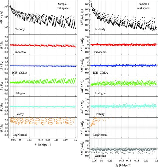
Average bispectrum (left-hand column) and its variance (right-hand column) for all triangle configurations obtained from the 300 realizations for the first mass sample in real space. The top panels show the results for the Minerva (black dots), while all other panels show the ratio between the estimate from an approximate method and the N-body one. In the last panel of the right-hand column the grey dots show the ratio between the Gaussian prediction for the bispectrum variance, equation (4), and the variance obtained from the N-body. The horizontal shaded area represents a 20 |${{\ \rm per\ cent}}$| error. The vertical lines mark the triangle configurations where k1 (the maximum of the triplet) is changing, so that all the points in between such lines correspond to all triangles with the same value for k1 and all possible values of k2 and k3. Since we assume k1 ≥ k2 ≥ k3, the value of k1 corresponds also to the maximum side of the triangle. Mocks for PeakPatch are not provided in the first sample so its bispectrum is missing in this case.
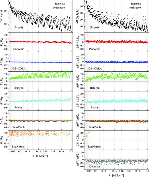
Same as Fig. 1, but for Sample 2.
All predictive methods, that is Pinocchio, ICE-COLA, and PeakPatch (this last for Sample 2), reproduce the N-body measurements within 15 per cent for most of the triangle configurations, with some small dependence on the triangle shape. Similar results, among the methods requiring some form of calibration, are obtained for Patchy, with just some higher discrepancies at the 20–30 per cent level appearing for Sample 2 at small scales, mainly for nearly equilateral triangles. The other calibrated methods fare worse. Halogen shows differences above 50 per cent, reaching 100 per cent for nearly equilateral configurations in both samples. The LogNormal approach, as one can expect, shows the largest discrepancy for all the scales and all the configurations in both samples.
Similar considerations can be made for the comparison of the variance. In this case a large component is provided by the shot-noise contribution, so the ratios to the N-body results show a less prominent dependence on the triangle shape. In general, we expect the agreement with N-body to depend to a large extent, particularly for Sample 2, on the correct matching of the object density, and more so for those LPT-based methods that show a lack of power in this regime. The Gaussian prediction underestimates the N-body result by 10–20 |${{\ \rm per\ cent}}$| for the majority of configurations, and reaching up to 50 per cent for squeezed triangles, i.e. those comprising the smallest wavenumber.
4.2 Redshift space
Figs 3 and 4, respectively, for Samples 1 and 2, show the redshift-space bispectrum monopole (left-hand column) and its variance (right-hand column), with the same conventions assumed for the real-space results in Fig. 1. The overall results are by and large very similar to the real-space ones. Only for the first sample, both Halogen and Patchy show a better agreement with the N-body results than in real space. As before lognormal is the one that shows the largest disagreement with the N-body results.
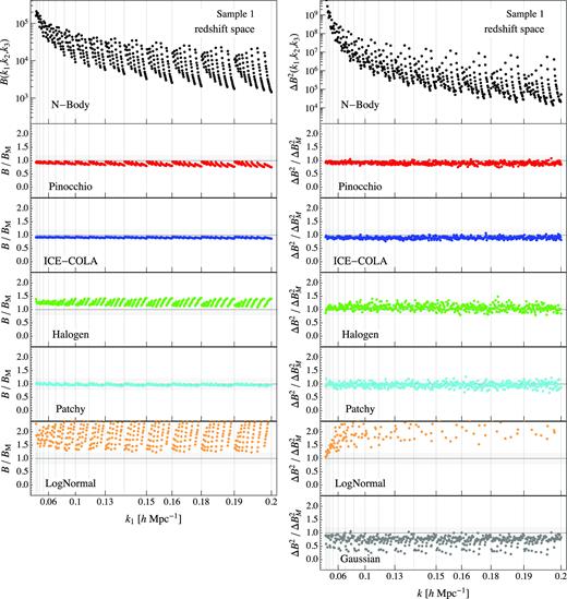
Average bispectrum (left-hand column) and its variance (right-hand column) for all triangle configurations obtained from the 300 realizations for the first mass sample in redshift space. The top panels show the results for the Minerva (black dots), while all other panels show the ratio between each a given estimate from an approximate method and the N-body one. In the last panel of the right-hand column, the grey dots show the ratio between the Gaussian prediction for the bispectrum variance, equation (4), and the variance obtained from the N-body. The horizontal shaded area represents a 20|${{\ \rm per\ cent}}$| error. The vertical lines mark the triangle configurations where k1 (the maximum of the triplet) is changing. Mocks for PeakPatch are not provided in the first sample so its bispectrum is missing in this case.
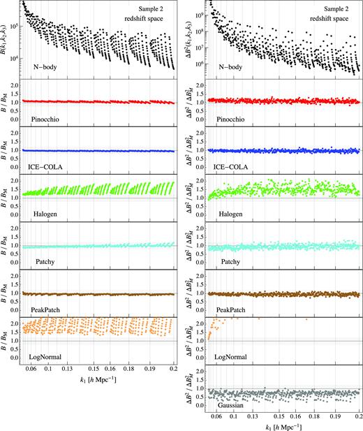
Same as Fig. 3, but for Sample 2.
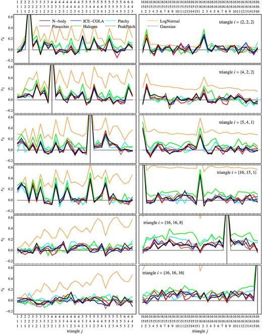
Cross-correlation coefficients rij for Sample 2, as defined in equation (6), for a choice of six triangles ti (one for each row) against two subsets of configurations at large and small scales (left- and right-hand columns, respectively) in redshift space. See the text for explanation.
The figure shows the correlation of six chosen triangles ti with two subsets of configurations tj: one at large scale tj = {1, 1, 1}Δk… {6, 4, 3}Δk and one at small scales tj = {16, 15, 1}Δk… {16, 16, 16}Δk, as explicitly denoted on the abscissa in terms of triplets in units of Δk.
With the exception of the diagonal cases ti = tj, most of the features in the rij plots reflect random fluctuations rather than actual correlations since 300 realizations are not sufficient to accurately estimate the bispectrum covariance matrix. A more accurate estimation of the matrix itself, limited to a single method, is presented in Section 6, where we show how such fluctuations are of the same order of the expected correlations among triangles sharing, for instance, one or two sides, and it is therefore impossible to tell them apart in this figure. Nevertheless, the random noise itself in the off-diagonal elements of the N-body covariance matrix is well reproduced by all approximate methods matching the initial conditions of Minerva (i.e. all except the lognormal case), with just slightly larger discrepancies from the Halogen estimate.
We obtain very similar results for Sample 2, with larger discrepancies (roughly by a factor of 2) for the Halogen and lognormal predictions.
5 COMPARISON OF THE ERRORS ON COSMOLOGICAL PARAMETERS
In addition to the direct comparison of bispectrum measurements and their estimated covariance, we explore, as done in Papers I and II, the implications for the determination of cosmological parameters of the choice of an approximate method.
In this case we will consider a simpler likelihood analysis, compared to those assumed for the 2-point correlation function and the power spectrum in the companion papers. In the first place, the model for the halo bispectrum, described in Section 5.1, is a tree-level approximation in PT and we will only consider its dependence on the linear and quadratic bias parameters, along with two shot-noise nuisance parameters. We also only consider the redshift-space bispectrum monopole as the implementation and testing of loop-corrections to the galaxy bispectrum in redshift space is well beyond the scope of this work.
In a first test, Section 5.3, we will include in the likelihood only the estimate of the bispectrum variance, since 300 realizations are insufficient for any solid estimation of the covariance of more than 500 triangular configurations, as originally measured. In Section 5.4, however, we consider a rebinning of these measurements that reduces the number of relevant configurations to less than a hundred and we will attempt a likelihood analysis involving the full-bispectrum covariance. While the chosen wavenumber bin in this case is likely too large for a proper bispectrum analysis, it should allow, to some extent, comparison of different estimates of the bispectrum covariance matrix. We will explore quantitatively the implications of a limited number of realizations and the relative approximations in Section 6.
We will not consider any study of the cross-correlation between power spectrum and bispectrum measurements, leaving that subject for future work.
5.1 Halo bispectrum model
We assume a tree-level model both for the matter bispectrum and for the halo bispectrum.
The model above will therefore depend on five parameters: the local bias parameters b1, b2, the nonlocal bias parameter γ2 and two shot noise parameters |$B^{(1)}_{\mathrm{ SN}}$| and |$B^{(2)}_{\mathrm{ SN}}$|. We will evaluate all matter correlators for our fiducial cosmology, along with the growth rate f, and consider them as known in our analysis.
The fiducial values of b1 for the two samples come from the comparison of the linear matter power spectrum and the halo power spectrum measured in the Minerva realizations. The quadratic bias b2 is in turn obtained from the linear one by means of the fitting formula in Lazeyras et al. (2016) while for the non-local bias γ2 we adopt the Lagrangian relation γ2 = −2/7(b1 − 1) (Chan et al. 2012).
We expect this model to accurately fit simulations over a quite small range of scales, typically for |$k\lt 0.07 \, h \, {\rm Mpc}^{-1}$| (see e.g. Sefusatti, Crocce & Desjacques 2012; Saito et al. 2014; Baldauf et al. 2015). However, we assume it to represent a full model for the halo bispectrum down to |$0.2\, h \, {\rm Mpc}^{-1}$| since we are merely interested in assessing the relative effect of different estimate of the variance on parameter determination. The value of |$k_{\mathrm{ max}}=0.2\, h \, {\rm Mpc}^{-1}$| is, nevertheless, a reasonable estimate of the reach of analytical models, once loop corrections are properly included (Baldauf et al. 2015). We leave a more extensive investigation, including a joint power spectrum–bispectrum likelihood to future work.
5.2 Likelihood
Similarly to the analyses in Papers I and II, since we are not interested in evaluating the accuracy of the model we assume, but only to quantify the relative effect of replacing the variance estimated from the N-body realizations with those obtained with the approximate methods, we assume as ‘data’ the ‘model’ bispectrum evaluated at some fiducial values for the parameters, that is |$B_{\mathrm{ data}}=B_{\mathrm{ model}}(p_\alpha ^{*})$|. While this leads to a vanishing χ2 for the best fit/fiducial values, it still allows to estimate how the error on the parameters depends on the bispectrum covariance estimation.
5.3 Constraints comparison: variance
Fig. 6 shows the ratio between the marginalized error on each parameter pα obtained from the variance estimated with a given approximate method and the same marginalized error on the same parameter obtained from the variance estimated from the Minerva N-body set. Such ratio is shown as a function of the maximum wavenumber kmax assumed for the likelihood evaluation that defines as well the total number of configurations Nt according to equation (16). The left-hand column corresponds to Sample 1 while the right-hand column to Sample 2. The grey-shaded area represents a 10 |${{\ \rm per\ cent}}$| discrepancy between error estimates.
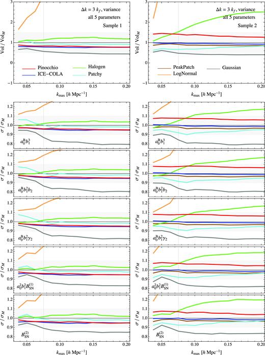
Marginalized errors for the model parameters obtained in terms of the redshift space bispectrum variance estimated with approximate methods compared with the errors obtained from the N-body estimate of the variance. First and second columns correspond, respectively, to Sample 1 and Sample 2. See the text for an explanation.
These results reflect those shown in the comparison of the variance. Unsurprisingly the methods that overestimate the variance lead to an overestimate of the error on each parameter, in a similar fashion across all parameters. As already shown in the previous figures, the predictive methods, along with Patchy, appear to be more accurate, with ICE-COLA, in particular, the one providing more consistent results for both samples. All such methods show discrepancies of less than 10 per cent w.r.t. the N-body case. The behaviour of Halogen is also quite good in the low-mass sample but the difference with N-body becomes larger than 10|${{\ \rm per\ cent}}$| in the second sample once small scales are included. LogNormal shows the largest difference, with reasonable results only for the very large scales. The Gaussian theoretical prediction provides a reasonable estimate at the largest scales while it underestimate the variance at small scales, particularly in the case of the parameters more directly related to bias, probably due to a missing non-Gaussian component.
Finally, Fig. 7, as an example, shows the 2σ contour plots for the parameters combinations pα in redshift space. Similar results are obtained for Sample 1. One can notice, in particular, that no method provides a variance estimate that affects the degeneracies between parameters in any specific way. Such effect might be more relevant when the full covariance is taken into account. We will comment on this in the next section.
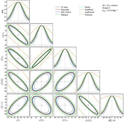
2σ contour plots for the parameters combinations pα (see the text) from the bispectrum monopole in redshift space for Sample 2. The constraints assume kmax = 0.2|$\, h \, {\rm Mpc}^{-1}$|. Notice that the N-body (black) results are plotted on top so that a few curves, corresponding to methods very closely reproducing the N-body, ones are not easily visible.
5.4 Constraints comparison: covariance
In this section we consider a comparison of the recovered parameters errors that accounts for the full covariance among triangular configurations. Clearly we need to reduce significantly the total number of triangles in order to recover reliable estimates of the covariance matrix even with our small set of independent realisations. We do so by rebinning our measurements in triangular configurations with sides defined by k-bins of size |$\Delta k = 6 k_f=0.025\, h \, {\rm Mpc}^{-1}$|. This is quite a large value leading to triangular bins, each accounting for a large set of fundamental triangles of quite different shape. For this reason it is probably not a good choice for a proper bispectrum analysis that aims at taking advantage of the different shape-dependence of the various contribution to the galaxy bispectrum. However, it can still provide a reasonable estimate of the covariance matrix, at least in the context of our comparison with N-body simulations.
As already mentioned, this binning choice leads to a total number of triangles of at most Nt = 86 for |$k_{\mathrm{ max}}=0.2\, h \, {\rm Mpc}^{-1}$|. We will then assume that their covariance matrix can be estimated reasonably well from the relatively small number of realizations available for each method and we can therefore compute the likelihood function in terms of equation (20). We do this for all possible values of kmax in steps of Δk. Notice that, despite the reduced number of triangular configurations, we correct the parameters covariance matrix by the factor shown in equation (18) of Percival et al. (2014) to take into account the uncertainty in the estimated inverse covariance.
The comparison of the individual marginalized errors is shown in Fig. 8. They are not too different from the previous one to the extent that most methods, and the predictive ones in the first place, do lead to errors within 10 per cent of those obtained from the N-body-based covariance on individual parameters. One can notice, however, a somehow larger discrepancy in the case of Halogen and a much larger one for the LogNormal estimate which is out of the shown interval in the case of the five-parameter volume comparison. On the other hand, the Gaussian theoretical prediction is responsible for an even more significant underestimate of the errors with respect to the previous case, as one can expect, at least in part, since it constitutes a diagonal approximation for the full covariance matrix.
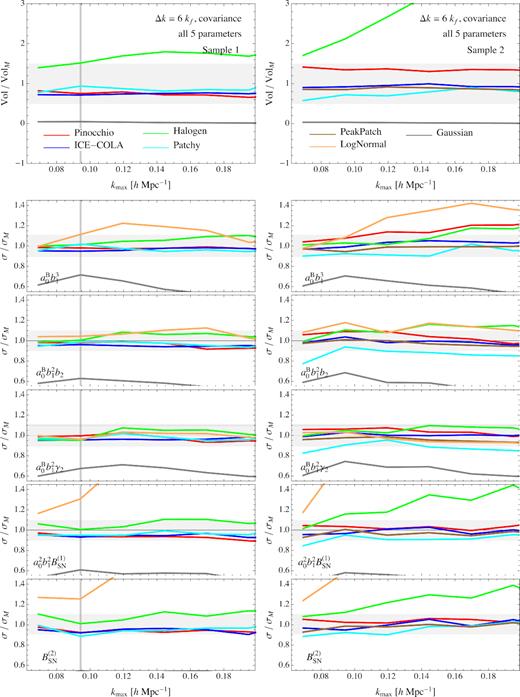
Same as Fig. 6 but assuming a k-bin of size Δk = 6kf and the full covariance matrix for all triangular configurations.
Fig. 9 shows the marginalized 2σ contours for pairs of parameters in the case of Sample 2 and |$k_{\mathrm{ max}}=0.2\, h \, {\rm Mpc}^{-1}$|. In addition to the considerations just made, one can observe how, in the context of the covariance comparison, different methods lead to slightly different degeneracies among the parameters, something not evident in the previous case of the variance comparison. Halogen, LogNormal, and the Gaussian (diagonal) prediction, in fact, stand out not only for the larger/smaller errors bars recovered but also for the degeneracies they provide for some couples of parameters.

Same as fig. 7 but assuming a k-bin of size Δk = 6kf and the full bispectrum covariance matrix.
6 TESTS WITH A LARGE SET OF REALIZATIONS
The number of 300 realizations, despite being quite a large number for many applications, is still rather small when it comes to estimate the covariance of hundreds or thousands of bispectrum configurations. For this reason we limited our likelihood comparisons to the bispectrum variance alone or, as an alternative, we used very large bins of wavenumber to reduce the number of triangles.
In this section we test the robustness of some of our conclusions taking advantage of a much larger sets of 10 000 Pinocchio catalogues characterized by the same configuration and cosmology as the 300 so far considered. In particular, this will allow us to investigate the relevance of the off-diagonal elements of the bispectrum covariance matrix for the two different binnings.
In Fig. 10 we show the ratios of the real-space bispectrum and its variance obtained from 300 realizations and the same quantities obtained from the 10 000 runs for both samples and for both binning choices. In the small-bin case the scatter on the bispectrum due to the limited number of runs is of the order of a few per cent, while for the variance is of the order of 10 per cent, with no particular dependence on shape. For the large bin the scatter is reduced below 1 per cent for the bispectrum and about at that level for its variance. Such differences are smaller than the discrepancies discussed among the results from different methods in the previous sections.
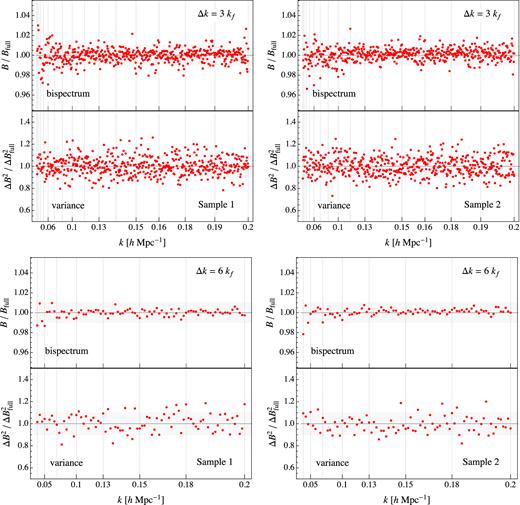
Ratio between the bispectrum and its variance as measured in 300 realizations of Pinocchio to the same quantities estimated from 10 000 realizations in real space. Top panels assumes Δk = 3kf, bottom panels Δk = 6kf. Sample 1 and Sample 2 are shown respectively in the left- and right-hand columns.
Fig. 11 shows a selection of elements from the rij, full matrix for the measurements assuming the bin Δk = 3kf and Sample 2. The two subsets of configurations on the abscissa correspond to triangles at the largest and smallest scales considered (respectively left- and right-hand columns) under the assumption of |$k_{\mathrm{ max}}=0.2\, h \, {\rm Mpc}^{-1}=16 \Delta k$|. It is interesting to notice how the noise characterizing the first estimates is of the order of the true off-diagonal correlations from the less noisy estimate, present, as expected, between configurations sharing one or two wavenumbers, e.g. ti = {2, 2, 2} and tj = {16, 15, 2}.
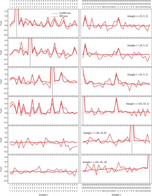
Cut through the cross-correlation coefficient in real space for all the triangle configurations coefficients estimated from 300 realizations (dashed line) and 10 000 realizations (continuous line) for the first sample. On the x-axis there are the triplets for each triangle in fundamental frequency unit. The cross-correlation coefficient is normalized to the Minerva variance.
Fig. 12 shows the same cross-correlation coefficients but for the larger binning, Δk = 6kf. Also in this the small-scale set of triangles corresponds to the configurations close to the limit of |$k_{\mathrm{ max}}=0.2\, h \, {\rm Mpc}^{-1}=8 \Delta k$|. The main difference with the previous case is the larger level of the correlations in the off-diagonal elements, due to the increased number of shared sides in the fundamental triangles falling in the larger triangular bins. The difference between the estimates from the 300 and 10 000 realizations sets is, however, smaller; in this case the off-diagonal structure of the covariance matrix is broadly reproduced even with 300 realizations, so this can be taken as a confirmation of the validity of the tests presented above.
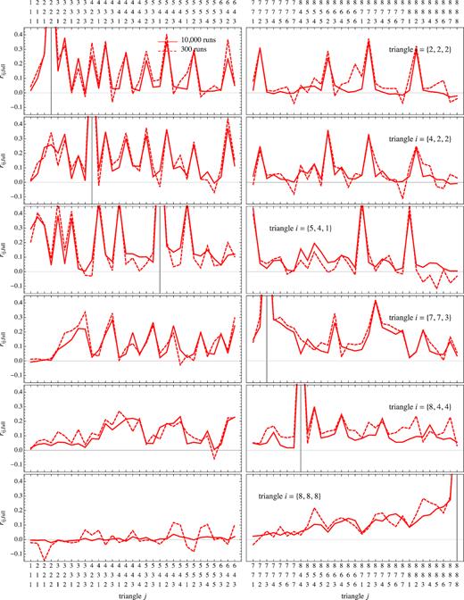
Same as Fig. 11 but with Δk = 6kf.
Finally, the top panels of Fig. 13 show the comparison between the volume error as defined in equation (22) for the five parameters pα obtained from the bispectrum variance estimated with 300 realizations, ‘Var(300)’ (the case adopted for the results in Section 5.3) and with the full set of 10 000 realizations, ‘Var(10,000)’ against the same quantity derived in terms of the covariance from all 10 000 runs, ‘Cov(10,000)’. We notice, in the first place, that no difference is noticeable in the results obtained from the variance estimated from the small or full sets. The difference between these and the case of the full covariance matrix is instead quite significant at almost all scales, except the very largest. In particular, for |$k_{\mathrm{ max}}=0.2\, h \, {\rm Mpc}^{-1}$|, the analysis based on the full covariance provides an error volume almost an order of magnitude larger w.r.t. the variance one, although, at the level of the marginalized errors on individual parameters (not shown) the difference is of the order of 10 per cent, i.d. comparable to the difference among the different methods.
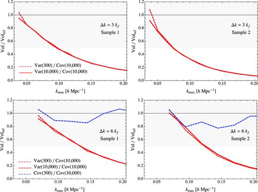
Errors volume, as defined in equation (22) for the bias parameters; in the top panel the case Δk = 3kf with the bispectrum variance from 10 000 realizations (continuous line) and the variance from 300 realizations (dashed line) compared with variance or the full covariance from 10 000; in the bottom panel the same but in the case Δk = 3kf with the additional dashed line accounting for the comparison between the full covariance matrix from 300 realizations and the full covariance matrix from 10 000 realizations. In the first column the results are shown for the first sample, in the second column for the second sample.
Similar results are shown, in the bottom panels of Fig. 13, for the large binning Δ = 6kf. In the case we can compute as well the covariance from the restricted set of 300 realizations, ‘Cov(300)’. The volume error in this case is still significantly smaller from the reference case by a 50 per cent at |$k_{\mathrm{ max}}=0.2\, h \, {\rm Mpc}^{-1}$|, but less than in the variance-based cases. As already done in Section 5.4, for this last comparison, we correct the parameters covariance in the ‘Cov(300)’ case by the factor shown in equation (18) of Percival et al. (2014) to take into account the small number of realisations used to estimate the covariance matrix when compared with the error measured from 10 000.
7 CONCLUSIONS
In this paper, and in its companions Papers I and II, we have studied the problem of covariance matrix estimation for large-scale structure observables using dark matter halo catalogues produced with approximate methods. This last paper, in particular, focuses on the halo bispectrum and its covariance matrix, with the twofold aim of assessing the correct reproduction of the non-Gaussian properties of the halo distribution as well as considering the halo/galaxy bispectrum as a direct observable in its own right.
The measurements are performed on sets of 300 (1000 for LogNormal) catalogues obtained from several different methods: ICE-COLA, PeakPatch, Pinocchio, Halogen, Patchy, and LogNormal, and they are compared with the reference Minerva suite of 300 N-body simulations. All approximate catalogues, apart from LogNormal, assume the same initial conditions of the full N-body simulations, thereby reducing differences due to cosmic variance. Out of each halo catalogue we select two samples characterized by a different minimal mass in order to gain a better perspective on our results as a function of mass and shot-noise levels.
The approximate methods can be generically subdivided into predictive methods (ICE-COLA, Pinocchio, PeakPatch), requiring a single redefinition of the halo mass to recover the expected halo number density, and methods (Halogen, Patchy), requiring as well a calibration of the bias function. It should be noted that, in the case of Halogen, such bias calibration is limited to the 2-Point Correlation Function and to configuration space, with only one parameter (per mass-bin) controlling the clustering amplitude. In addition, a third type is represented by the lognormal method, relying on a non-linear transformation of the matter density field, in turn calibrated on the halo mass function and halo bias. In all our analysis (with the exception of Appendix A) we have changed the limiting mass for each sample in order to ensure the same abundance for all catalogues, including those obtained with more predictive methods.
We have shown that:
the real space bispectrum is reproduced by ICE-COLA, Pinocchio, Patchy, and PeakPatch within 20 |${{\ \rm per\ cent}}$| for the most of the triangle configurations while Halogen and, particularly, lognormal present larger disagreements, often beyond 50 per cent;
these discrepancies are reflected on the results for the bispectrum variance, where, however, their systematic nature is less evident since there is no clear dependence on the triangle shape, probably due to the fact that for most triangles, the variance is dominated by the shot-noise component; the Gaussian prediction for the variance is generically underestimating the N-body result, particularly for squeezed triangles;
similar conclusions can be made for the redshift-space bispectrum monopole, where, however, Patchy and Halogen (the latter at least for the small mass sample) show a better agreement with the N-body simulations;
the inspection of the cross-correlation coefficients illustrates how, due to the matching initial conditions, almost all methods (except lognormal by construction) reproduce the noise present in the N-body estimation, which is dominating the off-diagonal elements of the covariance matrix estimated from only 300 realizations.
Our analysis was not limited to how accurately the bispectrum and its covariance are recovered, but include a comparison of the errors on cosmological parameters, in this case linear and non-linear bias parameters, derived from each approximate estimate of both the variance and the covariance of the halo bispectrum in redshift space. Since the relatively large set of 300 realizations is still not sufficient for a robust estimation of the full covariance of the hundreds of triangular configurations originally measured, we considered, in the first place, a likelihood analysis based on the bispectrum variance alone. In a second step, we rebinned the bispectrum measurements assuming a larger bin size for the wavenumber making up the triangle sides. This allows to reduce the overall number of triangle configurations to less than a hundred, allowing an estimate of their full covariance properties and the related likelihood analysis.
As in the similar analysis performed in the companion papers, we assumed a model for the bispectrum and produced a data vector from the evaluation of such model at some chosen fiducial value for the parameters. This allowed us to focus our attention exclusively on the errors recovered as a function of the different estimation of the covariance matrix. Differently from the companion papers, the model considered based on tree-level perturbation theory, only depends on bias and shot-noise parameters, allowing a much easier evaluation of the likelihood function. In particular, under these simplified settings we can easily compute our results as a function of the smallest scale, or maximum wavenumber kmax, included in the analysis. More rigorous tests involving additional cosmological parameters, a more accurate modelling of the redshift-space bispectrum in the quasi-linear regime, and a solid estimate of the full bispectrum covariance matrix (and cross-correlation with the power spectrum) are clearly well beyond the scope of this comparison project but will be required in the near future for the proper exploitation of the galaxy bispectrum as a relevant observable.
The parameter error comparison has shown that:
the error on the bias and on the shot-noise parameters are reproduced within 10|${{\ \rm per\ cent}}$| by all the methods except lognormal and Halogen in the high-mass sample for kmax > 0.07. This is evident as well in terms of the combined error volume as defined in equation (22); for the second sample Pinocchio and, to a lesser extent, Patchy, show an higher level of disagreement compared with the other predictive methods;
the Gaussian prediction tends to underestimate the error on some parameters for large values of kmax;
the two-parameter contour plots from the variance-based likelihood, for both mass samples and different values of kmax (not all shown in the figures), do not show any relevant difference among the methods in terms of parameter degeneracies; some differences in the recovered parameters degeneracies between the N-body and the Halogen, LogNormal, and, to a lesser extent Patchy results, are instead present in the case of the covariance-based likelihood.
To sum up, predictive methods, along with Patchy, appear to be the most accurate in reproducing the N-body results, but differences are overall relatively small. Of course, due to the relatively small number of N-body runs available, our likelihood tests have been either limited to include the bispectrum variance or forced to consider quite a larger k-bin, smoothing the shape dependence of the bispectrum and increasing the relevance of the off-diagonal elements of its covariance matrix. For this reason, we included additional tests employing 10 000 Pinocchio realizations to compare, at least for this particular method, the variance estimated from 300 realizations to the variance and the full covariance estimated from the whole set. This has shown that
the variance estimate is not particularly affected by the limited number of 300 runs and essentially no difference is found on the results for the parameters errors;
the results in terms of the full covariance, instead, do provide differences on the parameters errors but still within 10 per cent, although they highlight a progressive underestimate of the errors based on the variance alone beyond |$k_{\mathrm{ max}}\simeq 0.15 \, h \, {\rm Mpc}^{-1}$|, where a steady deviation proportional to kmax is observed.
Clearly, a more realistic investigation of the relevance of a reliable estimate of the bispectrum covariance matrix requires a proper model for the quasi-linear regime that we will leave for future work. In addition, we should also expect that the relatively small difference between the results obtained from the variance alone and the full covariance will become more relevant once a realistic window function is accounted for as beat-coupling/super-sample covariance effects are expected to provide additional contributions also to off-diagonal elements. Since such effects depend directly on the non-Gaussian properties of the galaxy/halo distribution, we consider the present work only as a first step toward a more complete assessment of the correct recovery of non-Gaussianity by approximate methods for mock catalogues.
From the analysis we have presented, it appears that most of the methods we considered are capable to reproduce the halo bispectrum, its variance, and the errors on bias parameters based on the variance alone quite accurately. This is particularly true for predictive methods such as ICE-COLA, Pinocchio, and PeakPatch. Similar results are obtained for Patchy, although the calibration in redshift space might lead to some larger systematic for the real-space bispectrum that in turn could have effects not investigated in this work (e.g. finite-volume effects). For what concern Halogen, we have already stressed that its calibration is restricted to the 2-point statistic so a lower accuracy on the bispectrum might be somehow expected. Nevertheless it is worth to point out that the marginalized errors on the parameters in redshift space, in particular for the first sample, are certainly comparable with all the other methods except for lognormal. This last method, in fact, is the one that fares worst among those considered. This is also not surprising since, as already mentioned, the non-linear transformation on the density field that provides a qualitatively reasonable description of the non-linear power spectrum, while providing a non-Gaussian contribution, does not ensure that such contribution, for instance in the case of the bispectrum, presents the correct functional form and dependence on the triangular configuration shape.
We notice finally how our tests on the bispectrum have highlighted differences among the different methods that are less evident from the similar analysis on 2-point statistic performed in the companion papers I and II. This illustrates how the bispectrum can be a useful diagnostic for this type of comparisons, even when we are not directly interested in the bispectrum as an observable. We expect that possible direction of investigation along these lines will include correlators of realistic galaxy distribution and, particularly for Fourier-space statistics, finite-volume effects, in order to better assess the interplay between non-Gaussianity, convolution with a window function and realistic shot-noise contributions.
ACKNOWLEDGEMENTS
We are grateful to the anonymous referee for a careful reading of the manuscript and, in particular, for suggesting the additional tests based on the full bispectrum covariance that, while not affecting the main outcomes of this work, significantly strengthen them.
M. Colavincenzo is supported by the Departments of Excellence 2018–2022 Grant awarded by the Italian Ministero dell’Istruzione, dell’Università e della Ricerca (MIUR) (L. 232/2016), by the research grant The Anisotropic Dark Universe Number CSTO161409, funded under the program CSP-UNITO Research for the Territory 2016 by Compagnia di Sanpaolo and University of Torino; and the research grant TAsP (Theoretical Astroparticle Physics) funded by the Istituto Nazionale di Fisica Nucleare (INFN). P. Monaco and E. Sefusatti acknowledge support from an FRA2015 grant from MIUR PRIN 2015 Cosmology and Fundamental Physics: Illuminating the Dark Universe with Euclid and from Consorzio per la Fisica di Trieste; they are part of the INFN InDark research group.
L. Blot acknowledges support from the Spanish Ministerio de Economía y Competitividad (MINECO) grant ESP2015-66861. M.Crocce acknowledges support from the Spanish Ramón y Cajal MICINN program. M. Crocce has been funded by AYA2015-71825.
M. Lippich and A.G.Sánchez acknowledge support from the Transregional Collaborative Research Centre TR33 The Dark Universe of the German Research Foundation (DFG).
C. Dalla Vecchia acknowledges support from the MINECO through grants AYA2013-46886, AYA2014-58308, and RYC-2015-18078. S. Avila acknowledges support from the UK Space Agency through grant ST/K00283X/1. A. Balaguera-Antolínez acknowledges financial support from MINECO under the Severo Ochoa program SEV-2015-0548. M. Pellejero-Ibanez acknowledges support from MINECO under the grant AYA2012-39702-C02-01. P. Fosalba acknowledges support from MINECO through grant ESP2015-66861-C3-1-R and Generalitat de Catalunya through grant 2017-SGR-885. A. Izard was supported in part by Jet Propulsion Laboratory, California Institute of Technology, under a contract with the National Aeronautics and Space Administration. He was also supported in part by NASA ROSES 13-ATP13-0019, NASA ROSES 14-MIRO-PROs-0064, NASA ROSES 12- EUCLID12-0004, and acknowledges support from the JAE program grant from the Spanish National Science Council (CSIC). R. Bond, S. Codis, and G. Stein are supported by the Canadian Natural Sciences and Engineering Research Council (NSERC). G. Yepes acknowledges financial support from MINECO/FEDER (Spain) under research grant AYA2015-63810-P.
The Minerva simulations have been performed and analysed on the Hydra and Euclid clusters at the Max Planck Computing and Data Facility (MPCDF) in Garching.
Pinocchio mocks were run on the GALILEO cluster at CINECA, thanks to an agreement with the University of Trieste.
ICE-COLA simulations were run at the MareNostrum supercomputer – Barcelona Supercomputing Center (BSC-CNS, http://www.bsc.es), through the grant AECT-2016- 3-0015.
PeakPatch simulations were performed on the GPC supercomputer at the SciNet HPC Consortium. SciNet is funded by the Canada Foundation for Innovation under the auspices of Compute Canada; the Government of Ontario; Ontario Research Fund – Research Excellence; and the University of Toronto.
Numerical computations with Halogen were done on the Sciama High Performance Compute (HPC) cluster which is supported by the ICG, SEPNet, and the University of Portsmouth.
Patchy mocks have been computed in part at the MareNostrum supercomputer of the Barcelona Supercomputing Center, thanks to a grant from the Red Española de Supercomputación (RES), and in part at the Teide High-Performance Computing facilities provided by the Instituto Tecnológico y de Energías Renovables (ITER, S.A.).
This work, as the companion papers, has been conceived and developed as part of the joint activity of the ‘Galaxy Clustering’ and the ‘Cosmological Simulations’ Science Working Groups of the Euclid survey consortium.
This paper and companion papers have benefited of discussions and the stimulating environment of the Euclid Consortium, which is warmly acknowledged.
Footnotes
REFERENCES
APPENDIX: MASS-CUT VS ABUNDANCE MATCHING
We have seen how predictive methods perform better overall than methods requiring calibration with a set of N-body simulations. However, all our results did assume, including predictive ones, that the halo density matches the one from the N-body catalogues to mach the halo density from the N-body catalogues. In this Appendix we compare the results presented so far and those obtained from Pinocchio, ICE-COLA, and PeakPatch when their predictions are taken out-of-the-box with no abundance matching. Since each method has a different definition of the mass, a constant mass cut will typically pick up different objects. This is especially true for PeakPatch halos that are defined as spherical overdensities in Lagrangian space and are not meant to reproduce FoF masses.
Fig. A1 shows the ratio of the bispectrum (left-hand column) and its variance (right-hand column) to the N-body results (similarly to Figs 3 and 4) in redshift space comparing the case of density matching (full colour) assumed so far to the case where the limiting mass is not changed (faded colour). Both mass samples are shown and we remind the reader that the PeakPatch catalogues are only available for Sample 2.
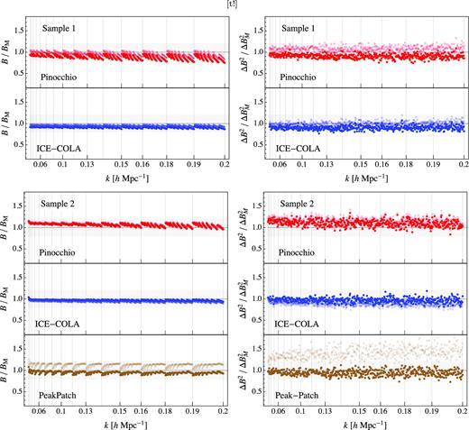
Bispectrum and its variance. Comparison of density matching (full colour) to mass-cut (faded colour), redshift space.
For the bispectrum the difference between the density matching and the mass-cut are lower than 10 |${{\ \rm per\ cent}}$| for Pinocchio and ICE-COLA for both the samples, while PeakPatch shows a larger difference, but always smaller than 20|${{\ \rm per\ cent}}$|, with density matching performing better as we can expect. For the variance the differences appear to be larger. ICE-COLA and Pinocchio present, respectively, differences of the order of 15–25 per cent for the first sample but smaller in the second sample case. PeakPatch, on the other hand, shows a difference of about 40 per cent for Sample 2.
Finally, Fig. A2 shows the combined error volume relative to the N-Body results, as in Fig. 6, for the two samples, comparing density matching (continuous lines) to the case of direct mass-cut (dashed lines). Using the measurements from the mass-cut case, for both samples, we recover larger errors, as can be expected from the variance comparison, with differences of the order of 10 per cent on the individual parameter error (50 per cent on the five-parameter volume shown in the figure) for Pinocchio. An even larger difference is found for PeakPatch, while discrepancies for ICE-COLA are within 5 per cent for both samples.
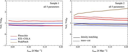
Marginalized errors for the bias parameters using the real bispectrum for the two samples (first and second columns) compared with the error obtained using Minerva. Density cuts are displayed with solid lines, while dashed lines represent mass cuts. The gray shaded area represents the 10|${{\ \rm per\ cent}}$| error on individual parameters, or 50 per cent on the five-parameter error volume.
