


ABSTRACT
The advent of new sub-millimetre (sub-mm) observational facilities has stimulated the desire to model the sub-mm line emission of galaxies within cosmological galaxy formation models. This is typically done by applying sub-resolution recipes to describe the properties of the unresolved interstellar medium (ISM). While there is freedom in how one implements sub-resolution recipes, the impact of various choices has yet to be systematically explored. We combine a semi-analytic model of galaxy formation with chemical equilibrium networks and numerical radiative transfer models and explore how different choices for the sub-resolution modelling affect the predicted CO, [C i], and [C ii] emission of galaxies. A key component for a successful model includes a molecular cloud mass–size relation and scaling for the ultraviolet and cosmic ray radiation field that depend on local ISM properties. Our most successful model adopts a Plummer radial density profile for gas within molecular clouds. Different assumptions for the clumping of gas within molecular clouds and changes in the molecular cloud mass distribution function hardly affect the CO, [C i], and [C ii] luminosities of galaxies. At fixed star formation rate, the [C ii]–SFR ratio of galaxies scales inversely with the pressure acting on molecular clouds, increasing the molecular clouds density and hence decreasing the importance of [C ii] line cooling. We find that it is essential that a wide range of sub-mm emission lines arising in vastly different phases of the ISM are used as model constraints in order to limit the freedom in sub-grid choices.
1 INTRODUCTION
Sub-millimetre (sub-mm) astronomy has grown significantly over the last decade with the advent of new and improved instruments such as the Atacama Large (sub-)Millimeter Array, the NOrthern Extended Millimeter Array, and the Large Millimeter Telescope. This field is expected to grow even further once new instruments such as the Cerro Chajnantor Atacama Telescope (CCAT)-prime and the currently discussed new instruments such as the next-generation Very Large Array and the Atacama Large-Aperture Submm/mm Telescope (AtLAST) come online. The quick rise in sub-mm collecting area and sensitivity has enabled the efficient collection of sub-mm emission-line information for large numbers of galaxies over cosmic time (see reviews by Carilli & Walter 2013; Casey, Narayanan & Cooray 2014).
At the same time, the available and expected observations from the newest generation of sub-mm facilities present a new and stringent challenge to theoretical models of galaxy formation. In particular, the rapidly growing number of CO (e.g. Daddi et al. 2010; Aravena et al. 2014; Tacconi et al. 2013; Walter et al. 2016; Decarli et al. 2016; Papovich et al. 2016; Tacconi et al. 2018), [C i] (e.g. Bothwell et al. 2017; Popping et al. 2017b), and [C ii] (e.g. Brisbin et al. 2015; Capak et al. 2015; Schaerer et al. 2015; Knudsen et al. 2016; Inoue et al. 2016) detections at z > 0 place a strong constraint on the interstellar medium (ISM) phase structure within galaxy formation models (see for a recent review Carilli & Walter 2013, and compilations presented in for example Olsen et al. 2017; Tacconi et al.2018). As a result, there has been significant interest within the galaxy formation community in modelling physics of these line emission processes within galaxy formation simulations.
The main challenges when predicting the sub-mm line emission from galaxy formation models is the large dynamic range of physical scales that have to be addressed. A successful model simultaneously needs to address galaxy baryonic physics acting on Mpc (or even larger cosmological scales), kpc, and pc scales for the distribution of matter within galaxies and the physics acting upon this matter, and atomic physics on sub-pc scales within molecular clouds. Combining these scales within one model is not computationally feasible, which has made theorists resort to ‘sub-resolution approaches’ (also called ‘sub-grid’). Developing these sub-grid approaches is not always straightforward and is usually based on either high-resolution idealized simulations or observations. In this paper, we do not discuss the sub-grid recipes invoked to describe physical processes acting on the baryons in galaxies [e.g. star formation (SF), stellar, and active galactic nuclei (AGNs) feedback, Somerville & Davé 2015. Instead we focus on the key sub-grid choices that are relevant in the context of modelling sub-mm line emission from galaxies in post-processing. This includes assumptions for the distribution and density profiles of molecular clouds, the radiation field, and the treatment of ionized gas.
Over the last decade multiple groups have focused on the modelling of sub-mm emission lines such as CO, [C i], and [C ii] from galaxies, either based on semi-analytic galaxy formation models (Lagos et al. 2012; Popping et al. 2014b, 2016; Lagache, Cousin & Chatzikos 2018), hydrodynamic models (Nagamine, Wolfe & Hernquist 2006; Narayanan et al. 2008; Narayanan et al. 2011, 2012; Narayanan & Krumholz 2014; Olsen et al. 2015a,b; Vallini et al. 2015; Olsen et al. 2017; Katz et al. 2017; Pallottini et al. 2017; Vallini et al. 2018), or analytic models (Narayanan & Krumholz 2017; Muñoz & Furlanetto 2013; Muñoz & Oh 2016). All these groups used a (cosmological) galaxy formation model as a starting point and combined this with machinery to model the sub-mm line emission of galaxies in post-processing. This machinery usually includes the coupling to a spectral synthesis code such as cloudy (Ferland et al. 2017) or a photodissociation region (PDR) code such as despotic (Krumholz 2013, 2014). An additional essential part of this machinery is the previously discussed sub-grid choices for the structure of the ISM. Sub-resolution choices ranging from imposed floor or fixed densities to varying density profiles (e.g. logotropic, Plummer, power-law and constant) to varying molecular cloud mass functions to diverse clumping factors have all been assumed within the literature (e.g. Lagos et al. 2012; Narayanan et al. 2012; Popping, Somerville & Trager 2014a; Popping et al. 2016; Olsen et al. 2017; Vallini et al. 2018).
Despite the wide range in assumptions that have been made for the sub-grid modelling, all these groups have successfully reproduced the sub-mm line emission of galaxies compared to observational constraints. This demonstrates that there is still a lot of freedom in the choices one can make for the sub-grid physics. These efforts have typically only focused on the emission from one molecule or atom (e.g. only CO or only [C ii] emission, although see Olsen et al. 2017; Pallottini et al. 2017). That said the emission from different atomic or molecular species can arise from drastically different ISM physical conditions. For example, 12CO (hereafter, CO) typically is associated with molecular H2 gas, while atomic [CI] can come from both molecular and neutral gas. Even more extreme is [CII] emission (emitted by singly ionized carbon, C+), which can reside cospatially with molecular, neutral, or ionized hydrogen. A model that successfully reproduces the [C ii] emission of galaxies therefore does not necessarily reproduce the emission from a molecular ISM tracer such as CO or HCN as well. Successfully reproducing the emission from multiple atoms and molecules simultaneously is therefore more challenging and has the potential to narrow down the freedom in designing the sub-grid approaches.
A systematic study of the typical choices made in sub-resolution modelling and their effect on the observed sub-mm line properties is thus important. In this paper, we explore how different sub-grid choices to represent the ISM in galaxies affect the resulting CO, [C i], and [C ii] emission of galaxies, while keeping the underlying galaxy formation model fixed (other works have also assessed the impact of some of their sub-resolution prescriptions, e.g. Olsen et al. 2017; Vallini et al. 2018). As a starting point, we use a semi-analytic model (SAM) of galaxy formation. We explore various sub-grid approaches to describe the distribution of diffuse and dense gas within the ISM of galaxies, especially focusing on the mass distribution function of molecular clouds, the density distribution profile within molecular clouds, clumping within molecular clouds, the ultraviolet (UV) and cosmic ray (CR) field impinging on molecular clouds, and the treatment of ionized gas. We combine chemical equilibrium networks and numerical radiative transfer models with sub-grid models to develop a picture of how the emission of CO, [C i], and [C ii] changes within galaxies. We aim to explore if the freedom in sub-grid assumptions can be limited when using a combination of multiple sub-mm emission lines as model constraints and try converge to a fiducial model that best reproduces the CO, [C i], and [C ii] emission of galaxies simultaneously. We do not aim to derive the characteristics (e.g. density profile) of giant molecular clouds in galaxies. We rather aim to find an operational prescription for the sub-mm emission of galaxies. Our conclusions about which model agrees best with observations are of course sensitive to the predicted ‘underlying’ properties from our particular SAM. While these conclusions may be fairly sensitive to the specifics of the galaxy formation model, the conclusions regarding how the details of the sub-grid modelling impacts the sub-mm line observables are robust.
This paper is structured as followed. In Section 2, we describe the model followed by a brief description of how different sub-grid choices affect the carbon chemistry in molecular clouds (Section 3). In Section 4, we describe the main results, while we discuss these in Section 5. We summarize our main results and conclusions in Section 6. Throughout this paper, we adopt a flat Λ cold dark matter cosmology with Ω0 = 0.28, |$\Omega _\Lambda = 0.72$|, |$h=H_0/(100\, \rm {km}\, \rm {s}^{-1}\, \rm {Mpc}^{-1}) = 0.7$|, σ8 = 0.812, and a cosmic baryon fraction of fb = 0.1658 (Komatsu et al. 2009) and a Charbier (Chabrier 2003) initial mass function.
2 MODELS
2.1 Galaxy formation model
We use the ‘Santa Cruz’ semi-analytic galaxy formation model (Somerville & Primack 1999; Somerville, Primack & Faber 2001) as the underlying galaxy formation model in this paper. Significant updates to this model are described in Somerville et al. (2008, 2012), Porter et al. (2014), Popping et al. (2014a, from here on PST14), and Somerville, Popping & Trager (2015, from here on SPT15). The model tracks the hierarchical clustering of dark matter haloes, shock heating, and radiative cooling of gas, SN feedback, SF, AGN feedback (by quasars and radio jets), metal enrichment of the ISM and intracluster medium, mergers of galaxies, starbursts, the evolution of stellar populations, the growth of stellar and gaseous discs, and dust obscuration, as well as the abundance of ionized, atomic and molecular hydrogen, and a molecular hydrogen-based SF recipe. In this section we briefly summarize recipes that are important components of the model with regards to the modelling of sub-mm emission lines (recipes to track the ionized, atomic, and molecular hydrogen abundance and the molecule-based SF recipe). We point the reader to Somerville et al. (2008, 2012), PST14, and SPT15 for a more detailed description of the model.
For this work, we construct the merging histories (or merger trees) of dark matter haloes based on the extended Press–Schechter (EPS) formalism following the method described in Somerville & Kolatt (1999), with improvements described in S08. We prefer EPS merger trees in this work because they allow us to achieve high-mass resolution, useful to explore differences in the sub-grid approaches for low-mass galaxies (nearly identical results are obtained for our SAM when run on merger trees extracted from N-body simulations and on EPS merger trees; Lu et al. 2014; Porter et al. 2014). Haloes are resolved down to a minimum progenitor mass Mres of |$M_{\rm res} = 10^{10}\, \rm {M}_\odot$| for all root haloes, where Mres is the mass of the root halo and represents the halo mass at the output redshift. A minimum resolution of Mres = 0.01Mroot is imposed (see appendix A of Somerville et al. 2015 for more details on this minimum mass resolution). The simulations were run on a grid of haloes with root halo masses ranging from 5 × 10⁸ to |$5 \times 10^{14}\, \rm {M}_\odot$| at each redshift of interest, with 100 random realizations at each halo mass. We have kept the galaxy formation parameters fixed to the values presented in PST14 and SPT15.
2.2 Sub-mm emission-line modelling
We use despotic (Krumholz 2014) to model the chemistry and sub-mm line emission of individual molecular clouds. This work builds upon the framework described in Narayanan & Krumholz (2017). We model molecular clouds as radially stratified spheres, where each sphere is chemically and thermally independent from one another. Each cloud contains 25 zones, sufficient to produce converged results for the emergent [C ii], [C i], and CO luminosities. We describe the adopted density distribution within the clouds in the following section.
We compute the chemical state of each zone using a reduced carbon–oxygen chemical network (Nelson & Langer 1999), in combination with a non-equilibrium hydrogen chemical network (Glover & Mac Low 2007; Glover & Clark 2012). The chemical reaction and their respective rate coefficients are summarized in table 2 of Narayanan & Krumholz (2017), and full details on the network are provided in Glover & Clark (2012). despotic requires the strength of the unshielded interstellar radiation field (GUV) and the CR primary ionization rate ξCR to iterate over the chemical network. The despotic implementation of the Glover & Clark (2012) network includes the effects of dust-shielding on the rates of all photochemical reactions. We describe how GUV and ξCR are calculated in the following section.
despotic iteratively solves for the gas and dust temperature and the carbon chemistry within each zone of the molecular clouds. It does this by considering the aforementioned chemical networks and a number of heating and cooling channels. The principal heating processes are heating by the grain photoelectric effect, heating of the dust by the interstellar radiation field, and CR heating of the gas. The cooling is dominated by line cooling, as well as cooling of the dust by thermal emission. Our model also includes cooling by atomic hydrogen excited by electrons via the Lyman α and Lyman β lines and the two-photon continuum, using interpolated collisional excitation rate coefficients (Osterbrock & Ferland 2006). Finally, there is collisional exchange of energy between dust and gas which becomes particularly relevant at relatively high densities (|$n\gtrsim 10^4$| cm−3). A full description of these processes is given in Krumholz (2014).
despotic solves for the statistical equilibrium within the level population of each atomic or molecular species. This is done using the escape probability approximation for the radiative transfer problem. despotic accounts for density variations within a zone due to turbulence, by including a Mach number-dependent clumping factor which represents the ratio between the mass- and volume-weighted density of the gas. It furthermore accounts for the cosmic microwave background (CMB) as a heating source as well as a background against which emission lines are observed (see for an extensive discussion on the importance of the CMB on sub-mm line emission for example da Cunha et al. 2013; Vallini et al. 2015; Olsen et al. 2017; Lagache et al. 2018). We refer the reader to Krumholz (2014) and Narayanan & Krumholz (2017) for a more detailed description of the despotic model and the adopted chemical networks. We use the Einstein collisional rate coefficient from the Leiden Atomic and Molecular Database (Schöier et al. 2005) for our calculations.
2.3 Sub-grid physics: coupling the Santa Cruz SAM to despotic
In this subsection, we describe the different assumptions we make to couple the Santa Cruz SAM to despotic. We divide the ISM in three phases, ionized, atomic, and molecular, as described in Section 2.1. The density distribution of the ISM in each modelled galaxy follows an exponential profile. We divide the gas into radial annuli and compute the fraction of molecular, atomic, and ionized gas as described above. For each annulus, we calculate the sub-mm line emission arising from the ionized, atomic, and molecular phase. The integrated sub-mm line emission from a galaxy is calculated by adding the contribution from each individual annulus. Our sub-grid approaches mostly focus on the molecular phase, but we will briefly address the atomic and ionized phases of the ISM towards the end of this section. A schematic overview of the coupling between the SAM and despotic is depicted in Fig. 1.
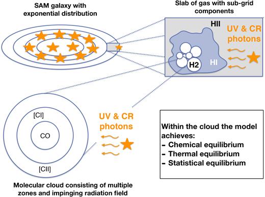
A schematic representation of the model presented in this work. Galaxies are represented by an exponential distribution of gas. An annulus of gas within a galaxy consists of ionized, atomic, and molecular gas. The molecular gas is made up by a number of molecular clouds sampled following a molecular cloud mass distribution function. Their sizes are set as a function of the molecular cloud mass and the external pressure acting on the molecular clouds. The individual molecular clouds are made up by radially stratified spheres illuminated by a far-UV (FUV) radiation field and CRs. The molecular clouds are not necessarily assumed to have a fixed average density, but can have a radial density profile. The initial abundance of carbon and oxygen in the ISM is set by the output of the SAM. Within every cloud, the model achieves chemical, thermal, and statistical equilibrium.
We want to emphasize that the sub-resolution models mark an operational prescription to bridge the gap in resolution between galaxy formation models (a SAM in this work) and the small-scale cloud physics. One could think of alternative prescriptions for the sub-resolution physics than presented in this work. Although interesting, exploring all possible options for each component of the sub-resolution model is a heroic effort too large for a single paper. We rather wish to limit ourselves to a number of well-defined variations in the sub-resolution prescriptions to demonstrate that the resulting sub-mm line emission predicted by models can be highly sensitive to even seemingly minor changes in the sub-resolution physics.
2.3.1 Molecular cloud distribution function
2.3.2 Molecular cloud size
The external pressure Pext is defined as Pext = Pm/(1 + α0 + β0), where α0 = 0.4 and β0 = 0.25 account for cosmic and magnetic pressure contributions (Elmegreen 1989; Swinbank et al. 2011). The pressure dependence is important, as it partially controls the density of the molecular clouds. In this paper, we will explore how the pressure dependence on the size of molecular clouds affects the sub-mm line luminosity of galaxies.
2.3.3 Density distribution functions within molecular clouds
We adopt four different approaches to model the density profile of gas within molecular clouds, a power-law density profile, a Plummer profile, a logotropic density profile, and a fixed average density. All these four profiles have been adopted in earlier works by different groups and we aim to explore the variation in the predicted sub-mm line luminosities between these density profiles. We describe the different profiles below and an example of each profile is given in Fig. 2. It becomes clear that the four different profiles can lead to significant differences in the minimum and maximum densities achieved within a molecular cloud and the radius out to which high-density gas (here loosely defined as densities larger than 1000 |$\rm {cm}^{-3}$|) is present. For all profiles we take |$n_{\rm H}(R \gt R_{\rm MC}) = 0\, \rm {cm}^{-3}$|. It can be expected that in reality individual giant molecular clouds follow a more complex hierarchical density structure. The four adopted profiles thus mark an operational definition for the density distribution within molecular clouds, (note that on top of this we account for turbulence driven variations in the densities as explained in Section 2.2). They should therefore be thought of as physically inspired, but not literal density distributions.
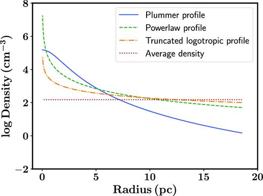
A representation of the four different density distribution functions within molecular clouds adopted in this paper. These were obtained assuming a molecular cloud with a mass of |$10^5\, \rm {M}_\odot$| and an external pressure acting upon this molecular cloud of |$P_{\rm ext}/k_{\rm B} = 10^4\, \rm {cm}^{-3}\rm {K}$|. One can clearly see the differences in minimum and maximum densities achieved in the inner and outer regions of the molecular cloud between the different profiles.
Fixed average density: the molecular clouds have a uniform density (i.e. a flat density profile) derived from their mass MMC and size RMC.
2.3.4 Impinging UV radiation field and cosmic ray strength
2.3.5 Elemental abundances
The elemental abundance of carbon [C/H] and oxygen [O/H] are scaled as a function of the gas phase metallicity of the cold gas Zc as predicted by the SAM, such that [C/H] =Zc × 2 × 10⁴ and [O/H] =Zc × 4 × 10⁴ (Draine 2011).
2.3.6 Contribution from the atomic diffuse ISM
Besides the molecular ISM, the atomic diffuse ISM may also contribute to the [C ii] emission of galaxies. To include the contribution from this ISM phase we model the atomic diffuse ISM as one-zone clouds. These clouds are illuminated by a UV radiation field and CR field strength scaled by the integrated SFR of the galaxy normalized by an SFR of |$1\, \rm {M}_\odot \, \rm {yr}^{-1}$| (|$G_{\rm UV} = G_{\rm UV,MW} \times \rm {SFR}$| and |$\xi _{\rm CR} = 0.1\, \xi _{\rm CR,MW}\times \rm {SFR}$|). These one-zone clouds have a column density of |$N_{\rm H} = 10\times 10^{20}\, \rm {cm}^{-2}$| and a hydrogen density of |$n_\text{H} = 10\, \rm {cm}^{-3}$| (Elmegreen & Elmegreen 1987; McKee, Parravano & Hollenbach 2015). The [C ii], [C i], and CO line-emission contribution by the atomic diffuse gas is added to the contribution by the molecular gas.
3 CARBON CHEMISTRY
Before presenting the CO, [C i], and [C ii] luminosity of galaxies when varying between different sub-grid recipes, we first explore how these choices affect the carbon chemistry (similar exercises have been performed before in e.g. Wolfire, Hollenbach & McKee 2010; Bisbas, Papadopoulos & Viti 2015; Bisbas et al. 2017).
In Fig. 3, we show the CO, [C i], and [C ii] abundance profile of a molecular cloud, as well as its temperature profile, when varying the density profile within the molecular cloud. For all these scenarios we assume a molecular cloud with a fixed mass of |$10^5\, \rm {M}_\odot$|, an external pressure acting upon of |$P_{\rm ext}/k_{\rm B} = 10^4\, \rm {cm}^{-3}\, \rm {K}$|, a UV radiation field of 1 G0, and a solar metallicity (at z = 0). We find that the different density profiles result in very different CO, [C i], and [C ii] abundance and temperature profiles. The Plummer density profile results in the largest mass fraction of CO, whereas adopting the fixed average density profile results in hardly any CO. The radius at which the [C i] abundance dominates varies significantly between the different density profiles. The gas temperature distribution is also very different between the different profiles. The gas temperature is highest at the edge of the molecular clouds when adopting the Plummer profile, but quickly drops to temperatures of |${\sim } 10\, \rm {K}$|.1 For the other profiles, we find a temperature of |${\sim } 30\, \rm {K}$| over a large fraction of the molecular cloud with a drop in temperature further inwards of the molecular clouds. Overall we find that the Plummer profile predicts much higher CO abundances and lower gas temperatures. The reason for this is that the Plummer profile has a long tail towards larger radii with relatively high densities (a few 1000 |$\rm {cm}^{-3}$|, see Fig. 2). This tail constitutes a large mass fraction and contributes significantly to the overall CO abundance and allows for efficient cooling of the gas.
![The [C ii] (top left), [C i] (top right), and CO (bottom left) abundance and gas temperature (bottom right) profiles of a molecular cloud for different molecular cloud density profiles. The molecular cloud has a fixed mass of $10^5\, \rm {M}_\odot$, an external pressure acting upon it of $P_{\rm ext}/k_{\rm B} = 10^4\, \rm {cm}^{-3}\, \rm {K}$, a UV radiation field shining on it of one G0, and a solar metallicity. The different density profiles lead to very different radial profiles for the CO, [C i], and [C ii] abundance and temperature of the gas.](https://oup.silverchair-cdn.com/oup/backfile/Content_public/Journal/mnras/482/4/10.1093_mnras_sty2969/1/m_sty2969fig3.jpeg?Expires=1749926986&Signature=f2REBDBGeI4-A0Twx52i28R11kEN4XUHEUIJUgdo7h5ioej9NYB5vnG71jhI8DF9SfwM3nObVkhWsHdgnMDFqN1f2WP5fRFY6uZDVOpwT~V78bMUru0GDILYBDPpOorFm5Vy6gqbMWZxM19ZANtM51B6q-1ZtbPjnays-VpM86e8RM2GMmWDuByqeGt89Ss1q0Q2MjUV482pSQqLeff4MpS3E-BkIQ8xg0VHyNhFyI-F4ClC~7vUA5MNJH41uD2xxKv-W-kJTGvHwRYBmcinJMI6V5F4y80Gi0bU1bYt36iCPEUXOzCHOQjAqWLMu4vVG7DYECD45xXufw5-2geA2A__&Key-Pair-Id=APKAIE5G5CRDK6RD3PGA)
The [C ii] (top left), [C i] (top right), and CO (bottom left) abundance and gas temperature (bottom right) profiles of a molecular cloud for different molecular cloud density profiles. The molecular cloud has a fixed mass of |$10^5\, \rm {M}_\odot$|, an external pressure acting upon it of |$P_{\rm ext}/k_{\rm B} = 10^4\, \rm {cm}^{-3}\, \rm {K}$|, a UV radiation field shining on it of one G0, and a solar metallicity. The different density profiles lead to very different radial profiles for the CO, [C i], and [C ii] abundance and temperature of the gas.
In Fig. 4, we show the CO, [C i], and [C ii] abundances of a molecular cloud when changing the external pressure acting upon the molecular cloud (molecular cloud properties are otherwise similar as in Fig. 3, assuming a Plummer density profile). As the pressure acting upon the molecular cloud increases, the density of the molecular cloud increases as well. As a result, a higher fraction of the carbon is locked up in CO, whereas the [C ii] abundance rapidly decreases. The increased density furthermore leads to a decrease in the gas temperature as a function of external pressure.
![The [C ii] (top left), [C i] (top right), and CO (bottom left) abundance and gas temperature (bottom right) profiles of a molecular cloud while varying the external pressure acting upon the molecular cloud. The molecular cloud has a fixed mass of $10^5\, \rm {M}_\odot$ distributed following a Plummer density profile, a UV radiation field shining on it of one G0, and a solar metallicity. As the external pressure increases, the CO abundances increases, whereas the [C ii] abundance decreases. The gas temperatures within the molecular cloud also decrease with increasing external pressure.](https://oup.silverchair-cdn.com/oup/backfile/Content_public/Journal/mnras/482/4/10.1093_mnras_sty2969/1/m_sty2969fig4.jpeg?Expires=1749926986&Signature=NmzB~nmsLZ5Bjlx8iuEBA4GoUZCTzs5Z4W3K5jlJFCxzkmtPEYcm~XPGYv-lGNbVqgzQgBVfLVf2NrfbI2DARJrGRq-qdBusXTYkfF0Yn2wmUdTxmOefGqX7DSKwkDPrwITMNf1CVHyWvQSyj~F7rGPJud8-7PP3QSnfNKctKae8ca1ocZ6yVWflzVi-3wVk~cnmsNhzKwenM3LlKRArbAurzv0UgrkKty6iVMXv3DNi9VsZBY01njOL5gExUwJecM9a4f6P1aAvUtYduOVj7dBEL1oKvNbZtj8uX7mgu6AFoESKb2KBtuvtJC2x8zs7FxetzTtSeW3-eIM~2-4ZUw__&Key-Pair-Id=APKAIE5G5CRDK6RD3PGA)
The [C ii] (top left), [C i] (top right), and CO (bottom left) abundance and gas temperature (bottom right) profiles of a molecular cloud while varying the external pressure acting upon the molecular cloud. The molecular cloud has a fixed mass of |$10^5\, \rm {M}_\odot$| distributed following a Plummer density profile, a UV radiation field shining on it of one G0, and a solar metallicity. As the external pressure increases, the CO abundances increases, whereas the [C ii] abundance decreases. The gas temperatures within the molecular cloud also decrease with increasing external pressure.
In Fig. 5, we show the CO, [C i], and [C ii] abundances of a molecular cloud when changing the UV radiation field (molecular cloud properties are otherwise similar as in Fig. 3, assuming a Plummer density profile). An increase in the UV radiation field results in a more effective dissociation of the CO molecules (e.g. Hollenbach, Takahashi & Tielens 1991; Wolfire et al. 2010), which lowers the CO abundance. Furthermore, the [C ii] abundance increases and the gas temperature increases.
![The [C ii] (top left), [C i] (top right), and CO (bottom left) abundance and gas temperature (bottom right) profiles of a molecular cloud for different strengths of impinging UV radiation field. The molecular cloud has a fixed mass of $10^5\, \rm {M}_\odot$ distributed following a Plummer density profile, an external pressure acting upon it of $P_{\rm ext}/k_{\rm B} = 10^4\, \rm {cm}^{-3}\, \rm {K}$, and a solar metallicity. As the strength of the UV radiation field increases, the [C ii] abundance and gas temperature become higher, whereas the [C i] and CO abundances are lower. Especially the temperature reacts very strongly on the strength of the UV radiation field, particularly in the regime where [C ii] dominates.](https://oup.silverchair-cdn.com/oup/backfile/Content_public/Journal/mnras/482/4/10.1093_mnras_sty2969/1/m_sty2969fig5.jpeg?Expires=1749926986&Signature=SQIvzrOfkzzwDCJjyM-mr523uOoy9YZXRGnJD8O7of9P9bbtcxiPp-XrmjOtLnoPD1t-xj21cxOpHrLJyEKwLl5FYIB8WiDQO-KdyoBkl~L4nQfnIg1fumYdPXVFlmPP1~6bHpW7YCKYr~JRJjx4iuzCk6klzbg8e-SVkO2eV-RQ2tgoiyOjmPHSqmB-kgRmACR3uTLuk9w~6Pqa7RPJdJL0V9qQvGFvro8nrXB2hnQtM7ZlbJCr9499AUHjRURHMrtGxJu4XBKr3qEFQp71EBn4A4SPzbIsRb5GYIlAB4PI9X9x4qU~9o0kvYJ8NZplt3Mmn~bdpZ53uD5NMzscvg__&Key-Pair-Id=APKAIE5G5CRDK6RD3PGA)
The [C ii] (top left), [C i] (top right), and CO (bottom left) abundance and gas temperature (bottom right) profiles of a molecular cloud for different strengths of impinging UV radiation field. The molecular cloud has a fixed mass of |$10^5\, \rm {M}_\odot$| distributed following a Plummer density profile, an external pressure acting upon it of |$P_{\rm ext}/k_{\rm B} = 10^4\, \rm {cm}^{-3}\, \rm {K}$|, and a solar metallicity. As the strength of the UV radiation field increases, the [C ii] abundance and gas temperature become higher, whereas the [C i] and CO abundances are lower. Especially the temperature reacts very strongly on the strength of the UV radiation field, particularly in the regime where [C ii] dominates.
Our results are in agreement with the findings by Wolfire et al. (2010) and Bisbas et al. (2015). For example, these authors also find that when the UV and/or CR field increases, the CO is more centrally concentrated within a molecular cloud.
4 CO, [C i], AND [C ii] LUMINOSITIES OF GALAXIES
In this section, we present our predictions for the CO, [C i], and [C ii] emission of galaxies, while varying the sub-grid components of our model. We restrict our analysis to central star forming galaxies, selected using the criterion sSFR > 1/(3tH(z)), where |$\rm {sSFR}$| is the galaxy specific star formation rate and tH(z) the Hubble time at the galaxy’s redshift. This approach selects galaxies in a similar manner to commonly used observational methods for selecting star-forming galaxies, such as colour–colour cuts (e.g. Lang et al. 2014). We present the 14th, 50th, and 86thpercentile of the different model variants in every figure. The 50thpercentile corresponds to the median, the 14thpercentile corresponds to the line below which 14 per cent of the galaxies are located, whereas the corresponds to the line below which 86 per cent of the galaxies are located. We typically only show the 14th and 86th for one model variant to increase the clarity of the figures. The scatter is always similar between the different model variants.
Throughout the rest of the paper, we will present our model predictions in four different plots, focusing on the [C ii], [C i], and CO emission of galaxies. [C ii] comparisons between model predictions and observations are performed using data presented in Brauher et al. (2008), de Looze et al. (2011), Cormier et al. (2015), and Díaz-Santos et al. (2017) at z = 0, Zanella et al. (2018) at z = 2, and a compilation of observations at z ∼ 6 (Capak et al. 2015; Knudsen et al. 2016; Willott et al. 2015; Decarli et al. 2017; González-López et al. 2014; Kanekar et al. 2013; Pentericci et al. 2016; Bradač et al. 2017; Schaerer et al. 2015; Maiolino et al. 2015; Ota et al. 2014; Inoue et al. 2016; Knudsen et al. 2017; Carniani et al. 2017). The comparison for [C i] is performed using z = 0 observations by Gerin & Phillips (2000). CO comparisons are carried out using data presented in Leroy et al. (2008), Papadopoulos et al. (2012), Greve et al. (2014), Kamenetzky et al. (2015), Liu et al. (2015), Cicone et al. (2017), and Saintonge et al. (2017) for z = 0, and Tacconi et al. (2010) and Tacconi et al. (2013) for z = 1 and 2. Infrared (IR) luminosities from the literature were converted into SFRs following the IR–SFR relation in Kennicutt & Evans (2012, comes from Murphy et al. 2011).
In some cases, the differences between the predictions by different sub-grid model variants are very minimal and are shown in the appendix rather than the main body of this paper.
4.1 Varying density profiles
In Fig. 6, we present model predictions for the [C ii] luminosity of galaxies as a function of their SFR at z = 0, 2, and 6. We show this for the four molecular cloud density profiles discussed in this work. We find that three of the four density profiles (Powerlaw, Logotropic, and Average) predict almost identical [C ii] luminosities for galaxies at all redshifts considered. The Plummer density profile predicts [C ii] luminosities that are approximately 0.5 dex lower than the other profiles, independent of redshift. The luminosities predicted by the Powerlaw, Logotropic, and Average density profiles are too high compared to the observations at z = 0 and 2 at z = 6 (except for a handful galaxies with an SFR of 10–100 |$\rm {M}_\odot \, \rm {yr}^{-1}$| and [C ii] luminosity brighter than |$10^{10}\, \rm {L}_\odot$| from Capak et al. 2015, note however that Faisst et al. (2017) suggest that the estimated SFRs of the Capak et al. sources are too low.). Overall, the model adopting the Plummer profile does best at reproducing the [C ii] luminosity of galaxies from z = 0 to 6. The fainter [C ii] luminosities predicted by the Plummer profile are driven by lower [C ii] abundances throughout most of the molecular cloud compared to the other density profiles (see Fig. 3).
![The [C ii] luminosity of galaxies as a function of their SFR at z = 0, 2, and 6, assuming different radial density profiles for the gas within molecular clouds. Model predictions are compared to observational constraints (Brauher, Dale & Helou 2008; de Looze et al. 2011; Cormier et al. 2015; Díaz-Santos et al. 2017; Capak et al. 2015; Knudsen et al. 2016; Willott et al. 2015; Decarli et al. 2017; González-López et al. 2014; Kanekar et al. 2013; Pentericci et al. 2016; Bradač et al. 2017; Schaerer et al. 2015; Maiolino et al. 2015; Ota et al. 2014; Inoue et al. 2016; Knudsen et al. 2017; Carniani et al. 2017; Zanella et al. 2018). In this particular plot, the Plummer model represents our fiducial model. Changing the density profile of molecular clouds can lead to variations up to ∼0.5 dex in the predicted [C ii] luminosity of actively star-forming galaxies.](https://oup.silverchair-cdn.com/oup/backfile/Content_public/Journal/mnras/482/4/10.1093_mnras_sty2969/1/m_sty2969fig6.jpeg?Expires=1749926986&Signature=29O6rJNNpBRhdckheH-tiia9xbaVxPBoNVky3ehm6Crt1E1MQ6~ZC7aXcRw1f1ozSPtlSuvEPiqGKVddGNL3kM8nheNBGTMDWsL7n1-8aeAhJbGouY9aES9tdi1VY182DGZxAxSuMRQj~bLwBuQD1Z1OpEiFjaHMmegPD4J-s~e1hEbo3YQWmYoFDdiag2AIbNjipmXL2zIWh1GNaQDAk2RnZAAuZL0SyNN7UdzYOVR1nndUv2oSh4~16Aqusx9OAX-zkeYAXBRZZBgrSYUY88R~mXlDrg3glss0dmlj9i3fK8AaCXaqAOJQOxPyIqPu0NqcikIDavKz88F1472r3g__&Key-Pair-Id=APKAIE5G5CRDK6RD3PGA)
The [C ii] luminosity of galaxies as a function of their SFR at z = 0, 2, and 6, assuming different radial density profiles for the gas within molecular clouds. Model predictions are compared to observational constraints (Brauher, Dale & Helou 2008; de Looze et al. 2011; Cormier et al. 2015; Díaz-Santos et al. 2017; Capak et al. 2015; Knudsen et al. 2016; Willott et al. 2015; Decarli et al. 2017; González-López et al. 2014; Kanekar et al. 2013; Pentericci et al. 2016; Bradač et al. 2017; Schaerer et al. 2015; Maiolino et al. 2015; Ota et al. 2014; Inoue et al. 2016; Knudsen et al. 2017; Carniani et al. 2017; Zanella et al. 2018). In this particular plot, the Plummer model represents our fiducial model. Changing the density profile of molecular clouds can lead to variations up to ∼0.5 dex in the predicted [C ii] luminosity of actively star-forming galaxies.
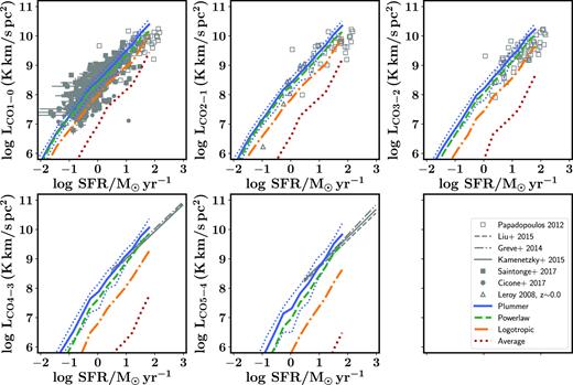
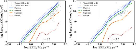
In Fig. 7, we show the predicted CO J=1–0, 2–1, 3–2, 4–3, and 5–4 luminosities of galaxies at z = 0 as a function of their SFR. Here again, the Plummer profile predicts luminosities significantly lower than the other three density profiles, up to almost an order of magnitude towards the most actively star-forming galaxies for all CO rotational transitions. The Logotropic and Average profiles predict CO luminosities that are a bit brighter than the Powerlaw profile. The Plummer profile predicts CO luminosities brighter than the other profiles for galaxies with an SFR less than |$1\, \rm {M}_\odot \, \rm {yr}^{-1}$|. Overall the Plummer profile best reproduces the CO J=1–0 through 5–4 luminosity of local galaxies over a large range in SFR. We find similar differences between the four density profiles when looking at the CO luminosities of z = 1 and 2 galaxies as a function of their SFR (Fig. 8). The Plummer density profile reproduces the CO luminosities of z = 1 and 2 galaxies best, whereas the other profiles predict CO luminosities ∼0.3 dex higher. The brighter CO emission predicted by the Plummer profile in galaxies with an SFR less than |$1\, \rm {M}_\odot \, \rm {yr}^{-1}$| is caused by the broad wing of the Plummer profile. This is clear in Fig. 2, where we see that for a cloud with a mass of |$10^5\, \rm {M}_\odot$| the Plummer profile predicts the highest densities from 1 to 5 pc. In Fig. 3, we then see that this indeed causes a higher CO abundance for a large fraction of the molecular clouds. This contribution makes a big difference in galaxies with low SFRs, which in the SAM are galaxies with lower gas surface densities and hence lower average volume densities.
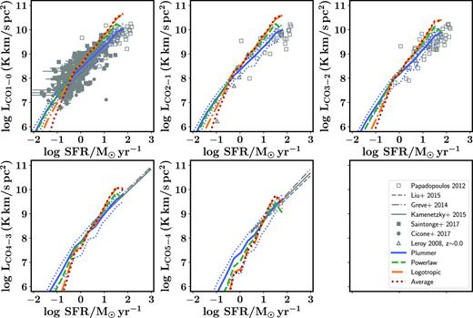
The CO J=1–0 to 5–4 luminosity of galaxies as a function of their SFR at z = 0 assuming different radial density profiles for the gas within molecular clouds. Model predictions are compared to observational constraints taken from Leroy et al. (2008), Papadopoulos et al. (2012), Cicone et al. (2017), Saintonge et al. (2017), Greve et al. (2014), Kamenetzky et al. (2015), and Liu et al. (2015). In this particular plot, the Plummer model represents our fiducial model. Changing the density profile of molecular clouds can lead to variations up to ∼0.5 dex in the predicted CO luminosity of galaxies.
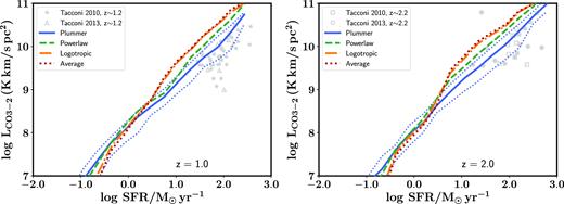
The CO J=3–2 luminosity of galaxies at z = 1 and 2 as a function of their SFR assuming different radial density profiles for the gas within molecular clouds. Model predictions are compared to observational constraints taken from Tacconi et al. (2010), and Tacconi et al. (2013). In this particular plot, the Plummer model represents our fiducial model. Changing the density profile of molecular clouds can lead to variations up to ∼0.5 dex in the predicted CO luminosity of galaxies. The Powerlaw, Logotropic, and Average density profiles predict CO luminosities that are too bright in z = 1 and 2 galaxies.
We present the [C i] 1–0 luminosity of galaxies at z = 0 as a function of their SFR in Fig. 9. There is only little difference between the Powerlaw, Logotropic, and Average model variants. The Plummer profile predicts [C i] 1–0 luminosities that are almost an order of magnitude fainter than the other model variants. Best agreement with the observations is found for the Plummer profile model variants.
![The [CI] 1–0 luminosity of galaxies at z = 0 as a function of their SFR assuming different radial density profiles for the gas within molecular clouds. Model predictions are compared to observational constraints taken from Gerin & Phillips (2000). In this particular plot, the Plummer model represents our fiducial model. Changing the density profile of molecular clouds can lead to variations up to 1 dex in the predicted [C i] luminosity of galaxies.](https://oup.silverchair-cdn.com/oup/backfile/Content_public/Journal/mnras/482/4/10.1093_mnras_sty2969/1/m_sty2969fig9.jpeg?Expires=1749926986&Signature=c9eh2s8amU49dT5yXnEq4P2nfQ~Wbea4qH9QgnN~9UQJbBBlXZilZJt9~TlUjNWPz4LfD~68ef4CAsb5eKOSjl368tWTRaZBjjo1168q0hUVgS~vx38kgu20gjKN45Iyy6t2Q1yr9IqhY5Qmwhcz8yiyUUhtjWyvuAlEe~DBtHGAYO-idz3Nn1NHzJQfin-z1mrJaHJNwDwck249gxXnVYFw-8C~8R9a1k3Gq7cmgqsQsjXzxDyrYynM4XoVtRy~3dBZtOBGzDUyjgkMq0v6r9QSzgFiSWsxPAol6IJWJkCO9eWLCO5L52mSETjD3p8pFf-vViWT9-QgyM2CPm3ntg__&Key-Pair-Id=APKAIE5G5CRDK6RD3PGA)
The [CI] 1–0 luminosity of galaxies at z = 0 as a function of their SFR assuming different radial density profiles for the gas within molecular clouds. Model predictions are compared to observational constraints taken from Gerin & Phillips (2000). In this particular plot, the Plummer model represents our fiducial model. Changing the density profile of molecular clouds can lead to variations up to 1 dex in the predicted [C i] luminosity of galaxies.
4.2 No pressure acting on molecular clouds
In this subsection, we explore the importance of the pressure dependence of the molecular cloud size for the sub-mm line luminosity of galaxies. In Fig. 10, we show the [C ii] luminosity of galaxies as a function of their SFR where we assume the external pressure is a constant |$P_{\rm ext}/k_{\rm B} = 10^4\, \rm {cm}^{-3}\, \rm {K}$| (the MW value for the external pressure). We find that the [C ii] luminosities predicted when adopting the various density profiles are all brighter than the observational constraints. The clear difference between observations and model predictions increases towards higher redshifts. At z = 0, the predictions by the Average, Logotropic, and Powerlaw profile are relatively similar. The Plummer profile predicts fainter [C ii] luminosities. The difference between the various profiles increases towards higher redshifts. Especially at z = 6, the model adopting the Average density profile predicts [C ii] luminosities that are significantly brighter than the other three variants. The physical cause of the bright [C ii] luminosities is twofold. First, the molecular clouds do not become smaller and denser in high-pressure environments, resulting in a larger ionized mass fraction of the cloud. Second, because the clouds are less dense, the mass of molecular hydrogen within the individual clouds is lower. The model therefore needs to sample more clouds from the cloud distribution function in order to equal the molecular hydrogen mass of the galaxy as calculated in equation (2). This increases the amount of [C ii] emission originating from molecular clouds. At z = 6, this even leads to unphysical situations for the model variant adopting the Average density profile. The total gas mass locked up in molecular clouds that is necessary to equal the molecular hydrogen mass dictated by equation (2) is larger than the total gas mass of the galaxy as predicted by the SAM.
![The [C ii] luminosity of galaxies as a function of their SFR at z = 0, 2, and 6 for different radial density profiles for the gas within molecular clouds and assuming a fixed external pressure acting on the molecular clouds of $P_{\rm ext}/k_{\rm B} = 10^4\, \rm {cm}^{-3}\, \rm {K}$. This figure is similar to Fig. 6, aside from the fact that here we impose a constant external pressure on clouds. When imposing a constant external pressure on the cloud the predicted [C ii] luminosities increase.](https://oup.silverchair-cdn.com/oup/backfile/Content_public/Journal/mnras/482/4/10.1093_mnras_sty2969/1/m_sty2969fig10.jpeg?Expires=1749926986&Signature=Ser3-MOYM4rtSV7bTXi5lEIUN3t16WX3SjDmYzgdEO8holA5SXQg1lIMVQHpNHxhIR~oSQE2aD2PAcQAJKOwaD0duD0uL-ygCt7cKP9sspT25enYO~f8fFKHoTEouh6vE2RTJVWBQDzUDaEIRWhcgCueiZIKuEo1sh3WNWbjUgoPkYH2KLmKcyoBryOrgISKMDlp3wFCsWPIAtQMV3lO7iV60qRtcu-q4GmW1TNPCsOFz~b1VbGq95PduM0DQac9UAK9YElToHs0wH45lYADeZGzL78-aF8vHlUpYx1NfV1iJZvB~jPlZpggC0qkNf3pE6jdS4HNHoRu0kY8RWLYow__&Key-Pair-Id=APKAIE5G5CRDK6RD3PGA)
The [C ii] luminosity of galaxies as a function of their SFR at z = 0, 2, and 6 for different radial density profiles for the gas within molecular clouds and assuming a fixed external pressure acting on the molecular clouds of |$P_{\rm ext}/k_{\rm B} = 10^4\, \rm {cm}^{-3}\, \rm {K}$|. This figure is similar to Fig. 6, aside from the fact that here we impose a constant external pressure on clouds. When imposing a constant external pressure on the cloud the predicted [C ii] luminosities increase.
For completeness, we present the predicted CO J=1–0 through 5–4 luminosity for z = 0 galaxies when assuming a constant |$P_{\rm ext}/k_{\rm B} = 10^4\, \rm {cm}^{-3}\, \rm {K}$| in Fig. 11. We find clear differences between the four different molecular cloud density profiles. The Powerlaw and Plummer density profiles are the only two that are still in agreement with the observations. The other two profiles predict CO luminosities that are much fainter. Especially, the Average profile predicts CO luminosities that are incompatibly low compared to observations. This difference increases for higher rotational CO transitions, indicating that the excitation conditions are different (with a fixed pressure the clouds are less dense and hence the low densities have a stronger effect on the high-J CO lines). We present the CO luminosity of higher redshift galaxies as a function of their SFR when assuming a constant |$P_{\rm ext}/k_{\rm B} = 10^4\, \rm {cm}^{-3}\, \rm {K}$| in Fig. 12. Similar to the CO luminosity of z = 0 galaxies we find that the Powerlaw and Plummer models still reproduce the observations. When adopting the other profiles the CO luminosities decrease, especially for the Average density profile. The difference becomes more dramatic for higher CO rotational transitions.
The CO J=1–0 to 5–4 luminosity of galaxies as a function of their SFR at z = 0 assuming different radial density profiles for the gas within molecular clouds and a fixed external pressure acting on the molecular clouds of |$P_{\rm ext}/k_{\rm B} = 10^4\, \rm {cm}^{-3}\, \rm {K}$|. This figure is similar to Fig. 7. When imposing a constant external pressure on the cloud the predicted CO luminosities decrease. This decrease is most dramatic and in strong tension with the observations for the Logotropic and Average density profiles. The CO luminosities predicted by the Plummer model variant are a little bit brighter.
The CO J=3–2 luminosity of galaxies at z = 1 and 2 as a function of their SFR assuming different radial density profiles for the gas within molecular clouds and a fixed external pressure acting on the molecular clouds of |$P_{\rm ext}/k_{\rm B} = 10^4\, \rm {cm}^{-3}\, \rm {K}$|. This figure is similar to Fig. 8. When imposing a constant external pressure on the cloud the predicted CO luminosities decrease. This decrease is most dramatic and in strong tension with the observations for the Logotropic and Average density profiles. The CO luminosities predicted by the Plummer model variant are a little bit brighter.
For three out of the four (Powerlaw, Logotropic, and Average) adopted density profiles the predicted CO luminosities decreased when fixing the external pressure to an MW value (most notably for the Logotropic and Average profile). This is driven by a decrease in the density of molecular clouds in high-pressure environment, changing the excitation conditions of CO as well. The Plummer profile variant is the only one for which the CO luminosities slightly increase when adopting a fixed MW external pressure. The reason for this is that the Plummer profile has a long tail towards larger radii with relatively high densities (a few 1000 |$\rm {cm}^{-3}$|, see Fig. 2). This tail constitutes a large mass fraction and contributes significantly to the overall CO abundance within molecular clouds, and hence the CO luminosity (Fig. 3). As the pressure increases, the fraction of the mass in this tail decreases.
In Fig. 13, we present the [C i] luminosity of galaxies when assuming |$P_{\rm ext}/k_{\rm B} = 10^4\, \rm {cm}^{-3}\, \rm {K}$|. We find that the [C i] luminosities predicted by the Powerlaw, Logotropic, and Average density profiles are almost identical. We furthermore find that the most actively star-forming galaxies have a [C i] 1–0 luminosity slightly brighter than the model variants where the external pressure is not set to the MW value.
![The [CI] 1–0 luminosity of galaxies at z = 0 as a function of their SFR assuming different radial density profiles for the gas within molecular clouds a fixed external pressure acting on the molecular clouds of $P_{\rm ext}/k_{\rm B} = 10^4\, \rm {cm}^{-3}\, \rm {K}$. This figure is similar to Fig. 9. When imposing a constant external pressure on the cloud the [C i] luminosities predicted by the various density profiles are almost identical.](https://oup.silverchair-cdn.com/oup/backfile/Content_public/Journal/mnras/482/4/10.1093_mnras_sty2969/1/m_sty2969fig13.jpeg?Expires=1749926986&Signature=ShfNoEhyCeQf01bDOSKMS1as1MeD~uz5hkJfJPsS0DR5vxN7zWvydziXPs9BEtw~lBgHgkUNYcMwYamiirBL~6fcQ2NcwyTBJrvEqfvN9SIyj38fIqKkaIONnscskbiDxNtS7ydqIDPkdKqACcrym580rpimrHJ0PL3c3gZfwYg7z6u1~JcPErA~zql6qEUddTRqEcUp2zsELx3~371k8IIdlnszAJ1JZB6i2DRAypSgD5tls1Cum~FoRn9niRC5Z23KVWscSrpnIwrxQqtO6TyA-0rL2-6y3amDYJeEsJaJESITf7XLk8oxIQTQeTPgDF3I28NhpRoOoG-yLvWfog__&Key-Pair-Id=APKAIE5G5CRDK6RD3PGA)
The [CI] 1–0 luminosity of galaxies at z = 0 as a function of their SFR assuming different radial density profiles for the gas within molecular clouds a fixed external pressure acting on the molecular clouds of |$P_{\rm ext}/k_{\rm B} = 10^4\, \rm {cm}^{-3}\, \rm {K}$|. This figure is similar to Fig. 9. When imposing a constant external pressure on the cloud the [C i] luminosities predicted by the various density profiles are almost identical.
Summarizing, we find that the increased external pressure in FIR bright galaxies leads to fainter predicted [C ii] and [C i] luminosities. It leads to brighter CO luminosities for the Powerlaw, Logotropic, and Average density profiles, and fainter CO luminosities for the Plummer profile. Overall we find that a model assuming a Plummer density profile where the size of molecular clouds depends on the external pressure acting on the molecular clouds reproduces best the available constraints for [C ii], [C i], and CO at low and high redshifts. In the remaining of the paper, we will use the Plummer-Pressure dependent model as our fiducial model to explore other sub-grid variations.
4.3 Turbulent compression of gas
Turbulence can cause a non-uniformity of the gas resulting in dense clumps within the ISM. The clumping factor represents the factor by which the mass-weighted mean density exceeds the volume-weighed mean density and is often approximated as a function of the Mach number of the gas (the ratio between the velocity dispersion and sound speed). This has been studied extensively in simulations of turbulent clouds (e.g. Ostriker, Stone & Gammie 2001; Federrath, Klessen & Schmidt 2008). In despotic, this is accounted for by an enhancement in the rates of all collisional processes (see for details Krumholz 2014). We show the effects of not including this turbulence-dependent clumping factor (i.e. clumping factor equals 1) in Appendix B. The [C ii] luminosities of galaxies at z = 0 predicted by the model that does not include turbulent compression of gas are ∼0.3 dex fainter than the luminosities predicted by our fiducial model variant that does include turbulent compression of gas. At higher redshifts, the difference is minimal. The CO emission predicted by the model variant that does not account for turbulent compression of gas are ∼0.1 dex fainter for CO J=3–2 and higher rotational transition in galaxies with SFRs less than 1 |$\rm {M}_\odot \, \rm {yr}^{-1}$|.
We note that the Plummer profile already guarantees a large range of densities within a molecular cloud, even without invoking a turbulence driven clumping factor. For the clumping to make a significant difference, the mass-weighted variance in density due to clumping must be larger than the variance implied by the Plummer density profile itself.
4.4 Molecular cloud mass distribution function
Our model assumes a slope for the molecular cloud mass distribution function of β = 1.8. In Appendix C, we examine the effects of changing this slope to β = 1.5 and 2.0, the range typically found for resolved nearby (Blitz et al. 2007; Fukui et al. 2008; Gratier et al. 2012; Hughes et al. 2013; Faesi et al. 2018). We find that the difference between the slope adopted in our fiducial model of β = 1.8 and 1.5, and β = 2.0 is negligible (Olsen et al. 2017).
4.5 UV radiation field and CRs
The UV radiation field and CR field strength acting on molecular clouds is important for the chemistry. We scale the CR and UV radiation field with the local SFR surface density. A different approach seen in the literature scales the CR and UV radiation field with the integrated SFR of galaxies (normalizing the SFR to |$1\, \rm {M}_\odot \, \rm {yr}^{-1}$|, e.g. Narayanan & Krumholz 2017). Fig. 14 shows our predictions for the [C ii] luminosity of galaxies for our fiducial model where the UV radiation field is normalized to the SFR surface density and a model where the UV radiation field is normalized to the integrated SFR of galaxies. At z = 0 and 2, the fiducial model predicts [C ii] luminosities that are slightly fainter in galaxies with an SFR less than |${\sim } 40\, \rm {M}_\odot \, \rm {yr}^{-1}$|. The fiducial model predicts fainter [C ii] luminosities for more actively star-forming galaxies, due to a quick rise in [C ii] luminosity as a function of SFR for the model variant based on the galaxy integrated SFR. At z = 6, it becomes clear that a model variant with a UV and CR field based on the integrated SFR of galaxies predicts a steeper slope for the [C ii]–SFR relation. We find that the model based on the integrated SFR of galaxies reaches poorer agreement with the z = 0 observations than our fiducial model, especially for the galaxies with the brightest FIR luminosities. This said, the prediction for the [C i] and CO luminosities of galaxies between our fiducial model and the model with CR and UV radiation field based on the integrated SFR are nearly identical (see Figs D1–D3 in Appendix D).
![The [C ii] luminosity of galaxies as a function of their SFR at z = 0, 2, and 6 for a model variant where the UV radiation field and CR strength are scaled as a function of the local SFR surface density (Fiducial) and as a function of the global galaxy SFR (UVSFR). This figure is similar to Fig. 6 aside from the varying relationship between the UV field and the SFR imposed in this figure. It is clear that a relationship that ties the UV field to the global SFR of galaxies underpredicts the [CII] luminosity at z = 0 for galaxies with an SFR less than $40\, \rm {M}\, \rm {yr}^{-1}$ and at high-redshift z = 6. It furthermore predicts [C ii] luminosities for z = 0 galaxies with SFRs higher than $40\, \rm {M}\, \rm {yr}^{-1}$ that are too bright. Tying the UV flux to ΣSFR results in predictions in good agreement with the observational constraints.](https://oup.silverchair-cdn.com/oup/backfile/Content_public/Journal/mnras/482/4/10.1093_mnras_sty2969/1/m_sty2969fig14.jpeg?Expires=1749926986&Signature=tTY3cy444h1mGrQlu1YO6TwX-~WN-OwXRstMQk02-AVpqoBc3CYNHgisBAf8wPIp5CKsEazKscTh23q75wb5NVmdPFk2a4Ofvt3m4DJqaHEShloPWJx~YrSP96Di-DIcoAcyKMh4XGhPYHJGUWeO7zP7so8kJrDJTFaVYjWn7Ul3Z~weR29uWKilkBmI7-njCojbFq9sAasPptlVhN6Go3E2Hi7A5LmMQ-sZIIMr7EubeB3z3HzSYbaLBQaYLOZF9X2eC3XqEn1gdSiSoBsDoNbHmqaNRn2UtjOIJ36lt3FTW8lugQ4mN9ZNX7lXuicXYdzrQREobkuzJalNBOpLmQ__&Key-Pair-Id=APKAIE5G5CRDK6RD3PGA)
The [C ii] luminosity of galaxies as a function of their SFR at z = 0, 2, and 6 for a model variant where the UV radiation field and CR strength are scaled as a function of the local SFR surface density (Fiducial) and as a function of the global galaxy SFR (UVSFR). This figure is similar to Fig. 6 aside from the varying relationship between the UV field and the SFR imposed in this figure. It is clear that a relationship that ties the UV field to the global SFR of galaxies underpredicts the [CII] luminosity at z = 0 for galaxies with an SFR less than |$40\, \rm {M}\, \rm {yr}^{-1}$| and at high-redshift z = 6. It furthermore predicts [C ii] luminosities for z = 0 galaxies with SFRs higher than |$40\, \rm {M}\, \rm {yr}^{-1}$| that are too bright. Tying the UV flux to ΣSFR results in predictions in good agreement with the observational constraints.
To explain why the [C ii] luminosity varies as a function of the UV and CR recipe, whereas the CO and [C i] luminosity do not, we focus in more detail on the chemistry within molecular clouds. We showed in Fig. 5 that as the strength of the radiation field increases, a larger fraction of total carbon mass is ionized and the fraction of carbon mass that is locked up in CO decreases. Based on this alone, one would expect that the [C ii] luminosity arising from a molecular cloud increases, whereas the CO and [C i] luminosities decrease. The bottom right panel of Fig. 5 shows that the temperature distribution within a molecular cloud changes dramatically as the strength of the impinging radiation field increases. A fainter CO or [C i] luminosity due to lower abundances is (partially) compensated by an increase in the temperature and the optical thickness of the cloud. For [C ii] on the other hand, the combination of a higher gas temperature and a larger [C ii] abundance results in even brighter luminosities. This enhancement in gas temperature is very significant in the regimes where most of the carbon is ionized (i.e. where the [C ii] abundance is significantly larger than the [C i] and CO abundances). We see this in Fig. A1, where we show the cumulative [C ii], [C i], and CO J=1–0 luminosity profile of a molecular cloud with a changing impinging radiation field (analogue to Fig. 5). Indeed, the [C ii] emission increases further into the cloud with increasing UV radiation. We find that the total [C i] and CO J=1–0 luminosity stay constant for G0 = 1 and 10 (and G0 = 100 for CO J=1–0). The final luminosity is reached further within the cloud as the UV radiation increases (due to changes in the abundance).
Our prediction that the CO and [C i] luminosity of galaxies stay roughly the same is in part because of a balance between abundance and gas temperature, but undoubtedly also by pure chance. A different sub-grid approach that results in a significantly weaker or stronger UV and CR radiation field does have the potential to predict CO and [C i] luminosities different from our fiducial model. The reason that a change in radiation field recipe is more notable in the [C ii] luminosities of galaxies is that the increase/decrease in gas temperature goes hand-in-hand with an increase/decrease of the [C ii] abundance.
4.6 Modelling the contribution from diffuse gas
So far we have focused on the sub-grid choices for the molecular gas in galaxies. The diffuse ISM can also contribute to the [C ii] emission of galaxies, especially in low-mass and low-SFR galaxies where the diffuse warm ISM constitutes a significant mass fraction of the ISM. Within our fiducial model, the atomic gas is modelled as a one-zone cloud with a mass density of |$10\, \rm {cm}^{-3}$|. In Fig. 15, we show the predicted [C ii] luminosity of galaxies for our fiducial model and a model variant where we assume the density of the atomic gas to be 1 and |$0.1\, \rm {cm}^{-3}$|, as well as model variants where we vary the column density of the one-zone clouds from 1019 to |$10^{21} \, \rm {cm}^{-2}$|.
![The [C ii] luminosity of galaxies as a function of their SFR at z = 0, 2, and 6 for our fiducial model variant, variants where the densities of the diffuse ISM are $1\, \rm {cm}^{-3}$ (IonizednH1) and $0.1\, \rm {cm}^{-3}$ (IonizednH0.1), and variants where the column density are 1019 (IonizedNH19) and $10^{21}\, \rm {cm}^{-2}$ (IonizedNH21), respectively. This figure is similar to Fig. 6. An increase in the density of the atomic diffuse ISM results in brighter [C ii] emission for FIR-faint galaxies at z = 0, but does not affect the [C ii] luminosities of z = 2 and 6 galaxies.](https://oup.silverchair-cdn.com/oup/backfile/Content_public/Journal/mnras/482/4/10.1093_mnras_sty2969/1/m_sty2969fig15.jpeg?Expires=1749926986&Signature=20BVErW1YPPu-AlSwpBX6d2cJ9QoeR4vbEjWglDPsmMJkU9Lo5eCPBgP8AXc5RrLWErjoNBDJJREb7AunpgJa5EtoG~6gEi8sAEQC6flhNQ7A2jAbVYq0agZ7ubN08SgARVF1BpxaIKws5bBdvs9BsWXZnhpRuEWQRvpd5ckwdIRwDfq2NNRibwqlQ9bR0Ci0OZHhP0KssCQaHlLudtN7jvzvy4uGugwS~2ec~NGjvUbZ~I-FUzRHX3n52OZM6Tlxm-JDqN--FxYGYhOnBU9jD5nEha64galEusvyNvzU~7Le-ABlzgF1kmro3D6pOoGyrvvMgjhxZhsvPABkYf4wA__&Key-Pair-Id=APKAIE5G5CRDK6RD3PGA)
The [C ii] luminosity of galaxies as a function of their SFR at z = 0, 2, and 6 for our fiducial model variant, variants where the densities of the diffuse ISM are |$1\, \rm {cm}^{-3}$| (IonizednH1) and |$0.1\, \rm {cm}^{-3}$| (IonizednH0.1), and variants where the column density are 1019 (IonizedNH19) and |$10^{21}\, \rm {cm}^{-2}$| (IonizedNH21), respectively. This figure is similar to Fig. 6. An increase in the density of the atomic diffuse ISM results in brighter [C ii] emission for FIR-faint galaxies at z = 0, but does not affect the [C ii] luminosities of z = 2 and 6 galaxies.
We find that lower densities for the atomic hydrogen results in fainter [C ii] emission for galaxies with low SFRs at z = 0. We find no significant difference between the different model variants at z = 2 and 6. This redshift dependence is driven by lower molecular hydrogen fractions in low-mass galaxies at z = 0 compared to higher redshifts (e.g. Popping et al. 2014a; Popping, Behroozi & Peeples 2015). No differences are found for the [C i] and CO emission of galaxies between the different model variants (see Appendix E). We find identical results between our fiducial model and a variant with a column density of |$10^{19} \, \rm {cm}^{-2}$| for the diffuse atomic gas. When adopting a column density of |$10^{21} \, \rm {cm}^{-2}$|, the model predicts fainter [C ii] emission in galaxies with SFRs below 1 |$\rm {M}_\odot \, \rm {yr}^{-1}$| at z = 0. At higher redshifts, the predicted [C ii] emission is identical to our fiducial model. As for changing the density of the gas, we find no significant different in the CO and [C i] emission of galaxies when adopting a different column density. This indicates that indeed the emission from atomic carbon and CO traces the molecular phase of the ISM. We do acknowledge that our sub-grid model for the atomic and ionized gas is very simplistic, and a more realistic model would account for density variations within the diffuse ISM (e.g. Vallini et al. 2015; Olsen et al. 2015b, 2017).
5 DISCUSSION
In this paper, we presented a cosmological model that predicts the [C ii], [C i], and CO emission of galaxies. Such models heavily rely on sometimes uncertain sub-grid choices to describe the ISM. In this work, we explored the effects of changing the sub-grid recipes on the [C ii], [C i], and CO emission of galaxies. We discuss the conclusions that can be drawn from our efforts.
5.1 Multiple emission lines as constraints for sub-grid methods
Throughout this paper, we have compared the predictions by the different model variants to observations of [C ii], [C i] 1–0, and multiple CO rotational transitions. As mentioned before, these different sub-mm emission lines originate in very different phases of the ISM, ranging from diffuse ionized gas to the dense cores of molecular clouds. We have seen that some model variants can for instance successfully reproduce the [C ii] emission of galaxies, but fail to simultaneously reproduce the CO emission of galaxies or the other way around (where a model assuming a fixed average density for molecular clouds and no pressure dependence on the size of molecular clouds most drastically fails to reproduce the CO luminosities of galaxies). It is only because multiple constraints are used that we can rule out these sub-grid model variants. This immediately brings us to the critical result of this paper: only by using a wide range of sub-mm emission lines arising in different phases of the ISM as constraints can the degeneracy between different sub-grid approaches be broken.
There are additional ways to constrain the degeneracy between different sub-grid approaches. Good examples of these are spatially resolved observations of individual molecular cloud complexes (e.g. Leroy et al. 2017; Faesi et al. 2018; Sun et al. 2018) and high-resolution simulations of molecular cloud structures. A clear census of the respective contribution by the diffuse and molecular ISM to the [C ii] emission can be obtained through the [N ii]-to-[C ii] ratio (Pineda, Langer & Goldsmith 2014; Decarli et al. 2014; Cormier et al. 2015). These are invaluable additional avenues to constrain the sub-grid methods typically adopted for works as presented in this paper.
5.2 Molecular cloud mass–size relation: the dominant sub-grid component
In our fiducial model, the size of a molecular cloud is set by a combination of the mass of the molecular cloud and the external pressure acting on this cloud. A higher external pressure results in a smaller size and therefore higher overall density within the molecular cloud. We found that this pressure dependence is essential to simultaneously reproduce the [C ii], [C i], and CO emission of galaxies over a large redshift range (see Section 4.2). We explored this for different radial density profiles for the gas within molecular clouds and found this statement to be true for all of the adopted density profiles. Of the four adopted profiles, the model variant adopting a Plummer density distribution within molecular clouds is the only one that can simultaneously reproduce the [C ii], [C i], and CO observational constraints. We will use this model variant (Plummer density profile in combination with a pressure dependence on the size of molecular clouds) in forthcoming papers to explore the sub-mm line properties of galaxies in more detail.
It is intriguing to realize that the simple recipe we adopted for the size of molecular clouds in combination with a Plummer density profile can reproduce the emission of sub-mm lines arising in different phases of the ISM over a large redshift range. We can also phrase this differently: a key requirement for successfully reproducing the sub-mm line emission of galaxies is a molecular cloud mass–size relation that varies based on the local environment of the molecular cloud (Field et al. 2011; Faesi et al. 2018; Sun et al. 2018).
Besides the importance of the external pressure acting on molecular clouds and the radial density dependence of gas within molecular clouds we have also explored the importance of turbulent gas within molecular clouds, the assumed molecular cloud mass distribution function, and different approaches to model the UV radiation field (and CR field strength) acting on the molecular clouds. A weaker/stronger radiation field changes the ionization depth within the molecular cloud. In particular, we find that a model that scales the impinging radiation field based on the local environment properties (in our case the local SFR surface density) rather than global properties better reproduces the available constraints on the [C ii] emission of galaxies. We do note that we have not explored ‘extreme’ scenarios where we increase or decrease the CR and UV radiation field strength by orders of magnitude. Such large differences have the potential to also significantly change the atomic carbon and CO abundance of gas within molecular clouds and therefore the resulting [C i] and CO emission lines.
5.3 Our fiducial model
In this paper, we converged to a fiducial model that best reproduces the [C ii], [C i], and CO properties of modelled galaxies within the framework of the underlying SAM. The key ingredients of this fiducial model include:
- The density distribution of gas within molecular clouds follows a Plummer profile, such that:where Rp is the Plummer radius, which is set to Rp = 0.1RMC. We account for additional clumping due to turbulence-driven compression of the gas (see Sections 2.2 and 4.3).(12)\begin{eqnarray*} n_{\rm H}(R) = \frac{3M_{\rm MC}}{4\pi R_{\rm p}^3}\biggl (1 + \frac{R^2}{R_{\rm p}^2}\biggr)^{-5/2}, \end{eqnarray*}
- The size of a molecular cloud depends on the molecular cloud mass, as well as the external pressure acting on the molecular cloud, such that:where kB is the Boltzmann constant.(13)\begin{eqnarray*} \frac{R_{\rm MC}}{\rm {pc}} = \biggl (\frac{P_{\rm ext}/k_{\rm B}}{10^4\, \rm {cm}^{-3}\rm {K}}\biggr)^{-1/4}\biggl (\frac{M_{\rm MC}}{290\, \rm {M}_\odot }\biggr)^{1/2}, \end{eqnarray*}
- The strength of the impinging UV radiation field scales as a function of the SFR surface density, such that:The strength of the CR radiation field also scales as a function of the SFR surface density (see equation 11).(14)\begin{eqnarray*} G_{\rm UV} = G_{\rm UV,MW} \times \frac{\Sigma _{\rm SFR}}{\Sigma _{\rm SFR,MW}}. \end{eqnarray*}
The diffuse atomic gas contributes to the [C ii] emission of a galaxy and is represented by one-zone clouds with a column density of |$N_{\rm H} = 10\times 10^{20}\, \rm {cm}^{-2}$| and a hydrogen density of |$n_\text{H} = 10\, \rm {cm}^{-3}$|.
5.4 Decreasing ratios between [C ii] and SFR: [C ii]–FIR deficit
Observations have suggested that the [C ii]–FIR ratio of galaxies decreases with increasing FIR luminosity, such that the FIR-brightest galaxies (|$L_{\rm FIR} \gt 10^{12}\, \rm {L}_\odot$|) have a [C ii]–FIR ratio 10 per cent lower than galaxies with fainter FIR luminosities (commonly known as the [C ii]–FIR deficit; Malhotra et al. 1997, 2001; Luhman et al. 1998, 2003; Beirão et al. 2010; Graciá-Carpio et al. 2011; Díaz-Santos et al. 2013; Croxall et al. 2012; Farrah et al. 2013). If we convert FIR luminosity into an SFR following Murphy et al. (2011), the same effect can be expected for the [C ii]–SFR ratio. An additional interesting feature of the [C ii]–SFR ratio, is that many z ∼ 6 galaxies have a [C ii]–SFR ratio much lower than one would expect from local [C ii]–SFR relations (e.g. Ota et al. 2014; Inoue et al. 2016; Knudsen et al. 2016).
We already noted in Section 4.2 that the [C ii] luminosity of actively star-forming galaxies is lower for our fiducial model than a model that assumes a fixed pressure acting of molecular clouds of |$P_{\rm ext}/k_{\rm B} = 10^4\, \rm {cm}^{-3}\, \rm {K}$| (compare Figs 6 and 10). In Fig. 16, we show again the [C ii] luminosity of galaxies as a function of their SFR predicted by our fiducial model. In this case, we include a colour coding that marks the mass-weighted external pressure acting on molecular clouds within each galaxy. We find a clear trend, where at fixed SFR the [C ii]–SFR ratio decreases with increasing external pressure. This is especially clear at z = 2 and 6, where the predicted [C ii] luminosities at fixed SFR can differ as much as two orders of magnitudes.
![The [C ii] luminosity of galaxies as a function of their SFR at z = 0, 2, and at z = 6 for our fiducial model, colour coded by the mass-weighted external pressure within galaxies acting on the molecular clouds. Note the clear decrease in [C ii] luminosity at fixed SFR as a function of increasing pressure.](https://oup.silverchair-cdn.com/oup/backfile/Content_public/Journal/mnras/482/4/10.1093_mnras_sty2969/1/m_sty2969fig16.jpeg?Expires=1749926986&Signature=lG0wSVHVTOKdW67RVWYw5z~LYJDXXFWzF6U~8Hgh1Vhn~kMMwdbNoYQNSZSYqz~WMV7ctBgH16lVJVDGwoQNT1a3WvCmgsR6wqeLy6FhbMqHwq5eJ6kXtHeNDFcpO7ESEVwq9sZ0izvDIPPY0WQ~Av1AAFbQcKnbXNsxy6JOkFzWTIhPvoSW2MbzCFTpMeLEv1EF9jf9JZiP-VuMP4-SAJjpcjp8njDP2czsB1nwvU1u-FUxwRbAWZgnBO8B1~QSYbfgOEBJSb9y4JiymaqCKT~VITQ~3ZClT6vVUhtMN2QS6J4scsvcBgGC9EozL27cTuHSob8QV5ZDoVwm5cZCYg__&Key-Pair-Id=APKAIE5G5CRDK6RD3PGA)
The [C ii] luminosity of galaxies as a function of their SFR at z = 0, 2, and at z = 6 for our fiducial model, colour coded by the mass-weighted external pressure within galaxies acting on the molecular clouds. Note the clear decrease in [C ii] luminosity at fixed SFR as a function of increasing pressure.
A decrease in the [C ii]–SFR ratio as a function of the external pressure is a natural result of our adopted molecular cloud mass–size relation, which also depends on the pressure acting on the molecular clouds. As the pressure increases, the clouds become smaller and the density increases as well. Because of the higher density a smaller mass fraction of the carbon is ionized, decreasing the [C ii] luminosity of the galaxies.
This result can (at least partially) explain the observed [C ii] deficit of local FIR-bright galaxies (e.g. Díaz-Santos et al. 2013) and the large number of non-detection of [C ii] in z ∼ 6 galaxies (e.g. Inoue et al. 2016). Increased densities in local mergers and high densities in high-z galaxies (in our framework driven by a high pressure environment) will naturally result in the [C ii] deficit and can explain the non-detections. We will explore this in more detail in a forthcoming paper, also focusing on variations in the C+ abundance and gas and dust temperatures along the [C ii] deficit.
5.5 A comparison to other works in the literature
5.5.1 Earlier work by Popping et al.
Popping et al. (2014a, 2016) also presented predictions for the CO, [C i], and [C ii] luminosities of galaxies based on the Santa Cruz SAM. For clarity, we briefly discuss the differences between those works and the work presented here, both in terms of methodology and model predictions.
Popping et al. (2014a, 2016) created a 3D realization of every modelled galaxy, assuming an exponential distribution of gas in the radial direction, as well as perpendicular to the galaxy disc. These works employed simple analytic approaches to calculate the abundance of CO, atomic carbon, and C+ and the temperature of the gas within every grid cell of the 3D realization. These (together with the density inferred from the exponential distribution) were then used as input for the radiative transfer calculations. It was assumed that a grid cell is made up by small molecular clouds all with a size of the Jeans length that belongs to the typical temperature and density of the grid cell. Individual molecular clouds were described by a one-zone cloud with a fixed density, accounting for turbulent compression of the gas.
The biggest differences in methodology compared to Popping et al. (2014a, 2016) are (1) the work presented in this paper only assumes an exponential distribution in the radial direction and does not have to make any assumption on the scale length of a galaxy disc in the z-direction, (2) the molecular mass within a galaxy is made up by sampling from a molecular cloud mass distribution function, (3) individual molecular clouds are not treated as one-zone models, but are allowed to have varying density profiles, (4) we use despotic to solve for the carbon chemistry and gas and dust temperatures rather than adopting simplified analytical solutions. Especially points 2–4 put the work presented in this paper on a more physics-motivated footing compared to Popping et al. (2014a, 2016).
In terms of model predictions, the biggest difference is that Popping et al. (2014a, 2016) were not able to reproduce the CO, [C i], and [C ii] emission of galaxies over a wide range of redshifts simultaneously. Our fiducial model does reproduce these simultaneously, marking the biggest improvement in model success.
5.5.2 Other cosmological models for the sub-mm line emission of galaxies
Lagos et al. (2012) presented predictions for the CO luminosity of galaxies based on a SAM. The authors parametrize galaxies with a single molecular cloud with a fixed density (a flat radial density profile), UV radiation field, metallicity, and X-ray intensity. They then use a library of radiative-transfer models to assign a CO line intensity to a modelled galaxy. The biggest difference between their approach and work presented here is that we describe individual galaxies by a wide range of molecular cloud with varying intrinsic properties (density, radiation field, and radius). This better captures the different conditions present in the ISM within a galaxy.
Lagache et al. (2018) used a SAM as the framework to make predictions for the [C ii] emission of galaxies. The authors use cloudy to calculate the [C ii] emission of molecular clouds. Lagache et al. (2018) also define a single PDR for each galaxy in their SAM, characterized by a mean hydrogen density (with a flat density profile), gas metallicity, and interstellar radiation field. The authors find [C ii] luminosities for galaxies at z > 4 similar to our findings, but have not explored other emission lines and lower redshift ranges.
Besides SAMs, a number of authors have made predictions for sub-mm emission lines based on zoom (high spatial resolution) hydrodynamic simulations (e.g. Narayanan et al. 2008, 2012; Olsen et al. 2015a,b; Vallini et al. 2016; Olsen et al. 2017; Pallottini et al. 2017; Vallini et al. 2018). Narayanan & Krumholz (2014) also used despotic to calculate the CO emission from molecular clouds. The authors adopt a flat radial density profile within molecular clouds and adopt a lower limit in the surface density of molecular clouds. This lower limit automatically ensures a large enough hydrogen/dust column to shield the CO. The authors find that as the SFR surface density of galaxies increases, the CO excitation also changes (higher-J CO lines are more excited). We have not specifically tested this result in our paper, but it is in line with our findings that a high pressure (due to higher gas surface densities which also cause higher SFR surface densities) increases the volume density of the ISM and allows for higher excitation of the high-J CO lines.
Vallini et al. (2018) post-process a zoom-cosmological simulation of one main-sequence galaxy at z = 6 (spatial resolution of 30 pc) to provide predictions for the CO line emission of this galaxy. Despite the high spatial resolution of this simulation, the authors still need to apply a sub-resolution model for the molecular cloud properties. Vallini et al. (2018) populate a sub-resolution element by individual molecular clouds with densities drawn from a lognormal density distribution with a power-law tail due to self-gravity. The width of the lognormal distribution is set by the Mach number of the gas. The CO radiative transfer is then solved using cloudy. The authors find that a high gas surface density (|$200\, \rm {M}_\odot \, \rm {pc}^{-2}$|), combined with a high Mach number and warm kinetic temperature of the gas lead to a peak in the CO spectral line energy distribution (SLED) at CO J=7–6. We have not shown predictions for the CO SLED of galaxies up to this excitation level, but the finding of an increased CO excitation with high gas surface densities and temperatures is in agreement with our general findings. The authors provide very detailed predictions for one object, an approach complementary to the semi-analytic effort focusing on large ensembles of galaxies.
Vallini et al. (2015) present predictions for the [C ii] luminosity of z = 6 galaxies as a function of IR luminosity, in agreement with the observed constraints. The authors find that the [C ii] luminosity of galaxies at a fixed FIR luminosity decreases as a function of metallicity. On top of this, we argue that changes in the ISM conditions (in our work a denser medium due to an increased external pressure upon molecular clouds) can naturally cause a change in the SFR–[C ii] ratio of galaxies. Pallottini et al. (2017) use the approach developed in Vallini et al. (2015) to make predictions for the [C ii] emission of a high-resolution zoom simulation of one galaxy at z = 6. They find that the [C ii] luminosity of this single galaxy is in agreement with the upper limits for the [C ii] luminosity of galaxies based on observations and in the same range as the [C ii] luminosity predictions of z = 6 galaxies presented in this work.
Olsen et al. (2015a) also post-process a hydro-zoom simulation to calculate the CO emission of three main-sequence galaxies at z = 2. The authors sample molecular clouds from a cloud-mass distribution function, similar to our approach. The authors then assign a size following a mass–size relation and also adopt a Plummer profile for the radial density distribution of molecular clouds. Olsen et al. (2015a) find CO luminosities in agreement with observations and similar to our findings. Like Vallini et al., the Olsen et al. work focuses on the resolved properties of individual galaxies which is a complementary approach to our efforts focusing on large groups of galaxies. Olsen et al. (2015b) additionally make predictions for the [C ii] emission of z = 2 galaxies based on cloudy calculations. The authors predict [C ii] luminosities similar to our predictions. Olsen et al. (2017) present predictions for the [C ii] emission of z = 6 modelled galaxies. Changes with respect to Olsen et al. (2015b) include updated cloudy calculations and the assumption of a logotropic density profile for the gas within molecular clouds. The authors predict [C ii] luminosities for ∼ 30 galaxies. The predicted [C ii] luminosity all fall well below expectations based on locally derived relations between SFR and [C ii] luminosity, as well as the predictions by our model.
5.6 Caveats
5.6.1 The diffuse ISM
In this work, we have implemented a very simplistic model for the sub-mm line emission arising in the diffuse ISM, consisting of a one-zone model with a fixed column depth. We demonstrated that different assumptions for the density of this diffuse gas can affect the [C ii] emission of galaxies, especially when the ISM is dominated by this diffuse phase (rather than ISM dominated by molecular gas, see Section 4.6). This immediately demonstrates the necessity of a more realistic representation of the diffuse ISM, at least accounting for a range in densities (see for example Olsen et al. 2017).
5.6.2 Unresolved galaxies
One of the intrinsic limitations of the semi-analytic method is the inability to spatially resolve galaxies. We therefore have to assume a profile for matter within galaxies, in this paper the commonly adopted exponential profile. In reality, the ISM of galaxies does not necessarily have to follow an exponential profile, especially in low-mass galaxies or at very high redshifts. Within our formalism a more concentrated distribution of gas would immediately increase the H2 fraction of the gas within galaxies as well as the pressure acting on molecular clouds and therefore the density within them. This naturally changes the carbon chemistry and excitation conditions.
We do want to emphasize that the choice for an exponential distribution of matter does not guarantee proper agreement between model predictions and observations. We furthermore wish to emphasize that a different distribution of matter within galaxies will also not change the differences we found between different sub-grid model variants. It is furthermore important to remember that models that do resolve the internal structure of galaxies (up to some extent) will have to rely on the same sub-grid methods as discussed in this work. Furthermore, many of these models do not reproduce galaxy internal structures (sizes and surface brightness distribution, see Somerville & Davé 2015, for a discussion).
5.6.3 X-rays and mechanical heating
We did not include X-rays as an additional heating source. The heating of X-rays on top of UV radiation and CRs can change the chemistry and excitation conditions of gas. Studies of the CO spectral line energy distribution in nearby active galaxies have indeed revealed strong excitation of high CO rotational transitions (CO J=9–8, van der Werf et al. 2010; Meijerink et al. 2013). Since we are only focusing on CO transitions up to CO J=5–4, it is not expected that X-ray heating strongly affects the luminosity of the sub-mm emission lines discussed in this work (Spaans & Meijerink 2008). An additional source of heating not discussed in this work is mechanical heating through shocks (Loenen et al. 2008; Meijerink et al. 2013; Rosenberg et al. 2014b,a).
6 CONCLUSIONS
In this paper, we presented a new cosmological galaxy formation model that predicts the [C ii], [C i], and CO emission of galaxies. We combined an SAM of galaxy formation with chemical equilibrium networks and numerical radiative transfer models. In this paper, we specifically explored how different choices for the sub-grid components affect the predicted [C ii], [C i], and CO emission-line strength of galaxies. Our main conclusions are as follows:
It is essential that a wide range of sub-mm emission lines arising in vastly different phases of the ISM are used as model constraints in order to limit the freedom in sub-grid approaches.
Small changes in the sub-resolution prescription for the ISM can lead to significant changes in the predicted CO, [C i], and [C ii] luminosities of galaxies.
The key requisite for a model that simultaneously reproduces the strength of multiple emission lines from galaxies in the local and high-redshift Universe is a molecular cloud mass–size relation that varies based on the local environment of the molecular clouds (in our framework as a function of the external pressure acting on molecular clouds).
A model that scales the impinging UV radiation field and CR field strength as a function of the local SF properties better reproduces the observational constraints for [C ii] than a model based on the integrated SFR of galaxies. Changes for the [C i] and CO luminosity of galaxies are minimal.
Not including clumping within molecular clouds and changing the slope for the cloud mass distribution function hardly affect the predicted [C ii], [C i], and CO luminosities for our fiducial model setup.
A successful model for the [C ii] emission of galaxies must include a realistic density distribution for the diffuse ISM.
A pressure dependence on the size of molecular clouds automatically causes a [C ii] deficit in high-pressure environments.
Our fiducial model successfully reproduces the [C ii], [C i], and CO emission of galaxies as a function of their SFR over cosmic time within the context of the current cosmological model predictions. This fiducial model includes a molecular cloud mass–size relation that additionally depends on the external pressure acting on a molecular cloud. It furthermore assumes a Plummer density profile within molecular clouds, and scales the UV and CR radiation fields as a function of the local SFR surface density. It assumes a molecular cloud mass distribution function with a slope of β = −1.8 and accounts for turbulence-driven clumping within molecular clouds. Lastly, it assumes a density for the diffuse atomic gas of |$10\, \rm {cm}^{-3}$|. This fiducial model can be used as a starting point for any group that wishes to model the sub-mm line emission from molecular clouds in galaxy formation simulations using a similar approach as presented in this work. Including these kind of approaches in models will increase the constraining power of sub-mm instruments for galaxy formation models and increase the informative role these models can play for future observations.
The prescriptions presented in this work do not represent a finite list of options. One could think of other approaches with an increasing level of complexity. When exploring other options, one should always take into account that minor changes in the sub-resolution physics can lead to large changes in the resulting emission from galaxies. These can best be constrained when focusing on as many emission lines simultaneously as possible.
ACKNOWLEDGEMENTS
GP thanks Karen Olsen for providing a [C ii] data compilation and for organizing the ‘Walking the line 2018’ conference which stimulated the creation of this work. GP thanks Anita Zanella for providing the [C ii] luminosities of z ∼ 2 galaxies prior to publication. The authors thank Romeel Davé, Gordon Stacey, and Chris Faesi for useful discussions and the referee for their comments that improved this work. DN was funded in part by grants from the US National Science Foundation via awards AST-1724864 and AST-1715206 and the Space Telescope Science Institute via award HST AR-13906.0001 and HST AR-15043.0001. RSS thanks the Downsbrough family for their generous support. The simulations in this paper were run on Rusty, supported by the Center for Computational Astrophysics, Flatiron Institute and on Draco, supported by the Max Planck Gesellschaft. Part of the writing of this manuscript was performed during an extended stay at the Munich Institute for Astronomy and Particle Physics as part of the workshop ‘The Interstellar Medium of High Redshift Galaxies’.
Footnotes
We note that the CMB sets a floor for the temperature of the molecular clouds which is above 10 K already at z = 2.7.
REFERENCES
APPENDIX A: THE LUMINOSITY PROFILE OF A MOLECULAR CLOUD
In this appendix, we show the [C ii], [C i], and CO J=1–0 luminosity profile of a molecular cloud as a function of the impinging radiation field. This is further discussed in Section 4.5.
![The cumulative [C ii] (left), [C i] (centre), and CO J=1–0 (right) luminosity profile of a molecular cloud for different strengths of the impinging UV radiation field. The molecular cloud has a fixed mass of $10^5\, \rm {M}_\odot$ distributed following a Plummer density profile, an external pressure acting upon it of $P_{\rm ext}/k_{\rm B} = 10^4\, \rm {cm}^{-3}\, \rm {K}$, and a solar metallicity. As the strength of the UV radiation field increases, the [C ii] luminosity increases, whereas for instance the total CO J=1–0 luminosity stays constant. The final CO J=1–0 luminosity is reached further within the cloud as the UV radiation field increases.](https://oup.silverchair-cdn.com/oup/backfile/Content_public/Journal/mnras/482/4/10.1093_mnras_sty2969/1/m_sty2969figa1.jpeg?Expires=1749926986&Signature=b0b6Imdo~~mkiG2xAUBLmV7tcD2AFWs0qvGtLtkzcDygzrXTdhGM9qqr5BBeK6Y-k0L-u4sB~QUkMrDaINRAa8ifIwHUHQoqaTSKSXtc8WvHdqzhltmkmXKZfSNX5CbveWcERVX54XSIya~ZXmpta4cRxXLPgKMhg17LgappF8vkSUg~yBMPFS7eJiODDLWaFGIEF8UlDQwziTDwkhyu13UvsxcJVt1drKKcnaxijthZ~sL0pUpiDC1q1847AlQd2JEA7p14O-ThmNXYkcEbkVlbtpZTTHwnS~RdQ4rNcy9de~nqbYGxNeyD-XnZXO85AkOhgyj4MWV233TbPmZtIA__&Key-Pair-Id=APKAIE5G5CRDK6RD3PGA)
The cumulative [C ii] (left), [C i] (centre), and CO J=1–0 (right) luminosity profile of a molecular cloud for different strengths of the impinging UV radiation field. The molecular cloud has a fixed mass of |$10^5\, \rm {M}_\odot$| distributed following a Plummer density profile, an external pressure acting upon it of |$P_{\rm ext}/k_{\rm B} = 10^4\, \rm {cm}^{-3}\, \rm {K}$|, and a solar metallicity. As the strength of the UV radiation field increases, the [C ii] luminosity increases, whereas for instance the total CO J=1–0 luminosity stays constant. The final CO J=1–0 luminosity is reached further within the cloud as the UV radiation field increases.
APPENDIX B: CLUMPING
In this appendix, we show the predicted [C ii], [C i], and CO luminosities of galaxies for a model variant in which clumping by turbulent gas motions is not taken into account and our fiducial model where this clumping is taken into account.
![The [C ii] luminosity of galaxies as a function of their SFR at z = 0, 2, and 6 for a model variant with (Fiducial) and without (NoClumping) turbulence dependent clumping. This figure is similar to Fig. 6. Clumping has a minimal effect on the predicted [C ii] luminosities of galaxies.](https://oup.silverchair-cdn.com/oup/backfile/Content_public/Journal/mnras/482/4/10.1093_mnras_sty2969/1/m_sty2969figb1.jpeg?Expires=1749926986&Signature=B~vCf1iFxvP-ygS4gop0VwDSM-8sNyoLj~-WoSHIt-rP7QdpZS9gyxkQpTew1PCzg-fv35U-vUZerHt4kPvkkje9~opVMwjG5BbztCgedSquy0kcga2evdDsrV2zFpeS-~ST1ZSBAeyx~6ALABiOtVGutb-xwK-5UUYNGAFcUk9-jiVApGx0vd1oyDANDNL2sYjUIEgftjU3Xdb3mhBo1yx-9B~jD-JmtGP9g4-OZ3Cux4HMW3gbgRE5TNNEvxLit-Y4pcefhr9gZnbpErk0HAa29C4oR2iXDwZjSMF~9oyDzpkhLRb1EsQnPReUA116p0TifrhkKUKwf4Nh-yntug__&Key-Pair-Id=APKAIE5G5CRDK6RD3PGA)
The [C ii] luminosity of galaxies as a function of their SFR at z = 0, 2, and 6 for a model variant with (Fiducial) and without (NoClumping) turbulence dependent clumping. This figure is similar to Fig. 6. Clumping has a minimal effect on the predicted [C ii] luminosities of galaxies.
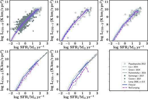
The CO J=1–0 to 5–4 luminosity of galaxies as a function of their SFR at z = 0 for a model variant with (Fiducial) and without (NoClumping) turbulence dependent clumping. This figure is similar to Fig. 7. The effect of clumping becomes more important for higher rotational CO transitions, however, this effect is small.
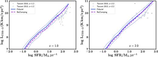
The CO J=3–2 luminosity of galaxies at z = 1 and 2 as a function of their SFR for a model variant with (Fiducial) and without (NoClumping) turbulence dependent clumping. This figure is similar to Fig. 8.
![The [CI] 1–0 luminosity of galaxies at z = 0 as a function of their SFR for a model variant with (Fiducial) and without (NoClumping) turbulence-dependent clumping. This figure is similar to Fig. 9. Clumping has a minimal effect on the predicted [C i] luminosities of galaxies.](https://oup.silverchair-cdn.com/oup/backfile/Content_public/Journal/mnras/482/4/10.1093_mnras_sty2969/1/m_sty2969figb4.jpeg?Expires=1749926986&Signature=jHRw0TbE-5IIBVw0PybTdBsNR45SxK~6SrK~XlmzSMDDOr8fY~QzELkgiIY4J6gSsNc-6WOuFASakMsEmL4H0uFITxcsEOKMEvmMTeZpt1x-FBx6~lwNMQFSAERsN7qT357qGSY2tWKbmwO8oJjMhTaJ8ey8SN8RYvWl16qAR2Nmfu8ojOvdi2L4IUaTRhwpu5SQki0IU3EPIpFmZj-zfcJaNTZny9JcR2m1T9zJuREx9jUo~GNsP~C91ib2vdcjoYjGdDRs5~K5w-kV0ZefiH8TAN4THly5QuI46Z9Lvdo7QQTLbcR-un12ciAfOfR8nNtsB3LlLsD2EI0TPR50uw__&Key-Pair-Id=APKAIE5G5CRDK6RD3PGA)
The [CI] 1–0 luminosity of galaxies at z = 0 as a function of their SFR for a model variant with (Fiducial) and without (NoClumping) turbulence-dependent clumping. This figure is similar to Fig. 9. Clumping has a minimal effect on the predicted [C i] luminosities of galaxies.
APPENDIX C: MOLECULAR CLOUD MASS DISTRIBUTION FUNCTION
In this appendix, we show the predicted [C ii], [C i], and CO luminosities of galaxies for model variants where we change the slope β of the molecular cloud mass distribution function from β = −1.5 to −2.0.
![The [C ii] luminosity of galaxies as a function of their SFR at z = 0, 2, and 6 for a model variant with a slope β of the cloud mass distribution function of β = 1.8 (Fiducial), β = 1.5 (slope1.5), and β = 2.0 (slope2.0). This figure is similar to Fig. 6. Different choices for the slope of the molecular cloud mass distribution function do not affect the predicted [C ii] luminosity of galaxies.](https://oup.silverchair-cdn.com/oup/backfile/Content_public/Journal/mnras/482/4/10.1093_mnras_sty2969/1/m_sty2969figc1.jpeg?Expires=1749926986&Signature=JcG87rtK4cduY~2vNg48n10KQqNHA1TNRE34ltwh0KOHPYpq8LMnrD~eh-cwVP~UgadKiVTNu5RfZv3ocUAKocbRYY4MO-YRRIijLZDvIQqpNUqidZr60dCS5-KT-sHBLFnY--78IcjTE8FGsGm2H9b0cU~VFuLrlV0uNLAJhtwdUWTZJAfu2RXbdp5FnRZgYehAQdD89lKuIiuKLJMcyut8sZystXMYwz1ngniWoxXZgrjdscUj3d804KxojbxmWkHjvGGbvD4-5F2cI8rRQQOwE9eAKKoSm6bPfRJGjZlFbp3E6Q5o9pr93aNQShN3vfpl8ve7wi7rhyxQT5ImCA__&Key-Pair-Id=APKAIE5G5CRDK6RD3PGA)
The [C ii] luminosity of galaxies as a function of their SFR at z = 0, 2, and 6 for a model variant with a slope β of the cloud mass distribution function of β = 1.8 (Fiducial), β = 1.5 (slope1.5), and β = 2.0 (slope2.0). This figure is similar to Fig. 6. Different choices for the slope of the molecular cloud mass distribution function do not affect the predicted [C ii] luminosity of galaxies.
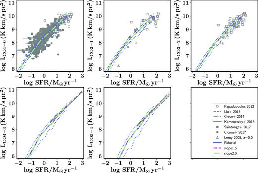
The CO J=1–0 to 5–4 luminosity of galaxies as a function of their SFR at z = 0 for a model variant with a slope β of the cloud mass distribution function of β = 1.8 (Fiducial), β = 1.5 (slope1.5), and β = 2.0 (slope2.0). This figure is similar to Fig. 7. Different choices for the slope of the molecular cloud mass distribution function do not affect the predicted CO luminosity of galaxies.
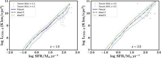
The CO J=3–2 luminosity of galaxies at z = 1 and 2 as a function of their SFR for a model variant with a slope β of the cloud mass distribution function of β = 1.8 (Fiducial), β = 1.5 (slope1.5), and β = 2.0 (slope2.0). This figure is similar to Fig. 8. Different choices for the slope of the molecular cloud mass distribution function do not affect the predicted CO luminosity of galaxies.
![The [CI] 1–0 luminosity of galaxies at z = 0 as a function of their SFR for a model variant with a slope β of the cloud mass distribution function of β = 1.8 (Fiducial), β = 1.5 (slope1.5), and β = 2.0 (slope2.0). This figure is similar to Fig. 9. Different choices for the slope of the molecular cloud mass distribution function to not affect the predicted [C i] luminosity of galaxies.](https://oup.silverchair-cdn.com/oup/backfile/Content_public/Journal/mnras/482/4/10.1093_mnras_sty2969/1/m_sty2969figc4.jpeg?Expires=1749926986&Signature=Qmo4Xf1AUG7dhHrpcOiOiQeBxWKjzLlgJvsieCDLcKooU8kRSHTrqdTUwcfOIbpfw8YOlX5tVRtPqKBzODj1dy9KpaLy1cAL4faVfwDlZIqn5PR8RjCWnVV2eMZ~Upgvk9NVtXBw7TB6XUArnTDCT~pAmPBLCTO~rd2Y61F5DmEuiiYaZPUxPp-EdP8FBBO-n4mp-OvYEOteYGifJmHEPth9TpM9aYQ5UUnpmyIgW8aZQf7hxjR7VhiPG10poIDNNiIRFjnDQUL8y1~nk3-2I4dZVPyZ-NTW-dqxqnSSw~89CUDv9-iL29sCWAKQQAo1v~vj2TOA0LftwS-P~GXMFg__&Key-Pair-Id=APKAIE5G5CRDK6RD3PGA)
The [CI] 1–0 luminosity of galaxies at z = 0 as a function of their SFR for a model variant with a slope β of the cloud mass distribution function of β = 1.8 (Fiducial), β = 1.5 (slope1.5), and β = 2.0 (slope2.0). This figure is similar to Fig. 9. Different choices for the slope of the molecular cloud mass distribution function to not affect the predicted [C i] luminosity of galaxies.
APPENDIX D: UV RADIATION FIELD AND CRS
In this appendix, we show the predicted [C i], and CO luminosities of galaxies for our fiducial model where the strength of the UV and CR field scale with the local surface density and a model variant where they scale with the integrated SFR of a galaxy.
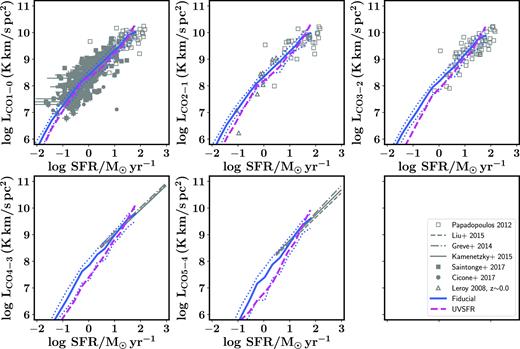
The CO J=1–0 to 5–4 luminosity of galaxies as a function of their SFR at z = 0 for a model variant where the UV radiation field and CR strength are scaled as a function of the local SFR surface density (Fiducial) and as a function of the global galaxy SFR (UVSFR). This figure is similar to Fig. 7. The CO luminosities predicted by the two different model variants to scale the UV and CR field are very similar.
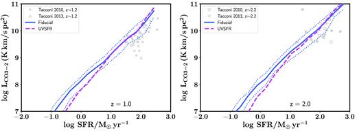
The CO J=3–2 luminosity of galaxies at z = 1 and 2 as a function of their SFR for a model variant where the UV radiation field and CR strength are scaled as a function of the local SFR surface density (Fiducial) and as a function of the global galaxy SFR (UVSFR). This figure is similar to Fig. 8. The CO luminosities predicted by the two different model variants to scale the UV and CR field are very similar.
![The [CI] 1–0 luminosity of galaxies at z = 0 as a function of their SFR for a model variant where the UV radiation field and CR strength are scaled as a function of the local SFR surface density (Fiducial) and as a function of the global galaxy SFR (UVSFR). This figure is similar to Fig. 9. The [C i] luminosities predicted by the two different model variants to scale the UV and CR field are very similar.](https://oup.silverchair-cdn.com/oup/backfile/Content_public/Journal/mnras/482/4/10.1093_mnras_sty2969/1/m_sty2969figd3.jpeg?Expires=1749926986&Signature=asPviR4Q~Ldt1aEdyNo8B5DGI~biizkssH2Gr~9L9kNgt~M6yOW3Wv0YaSNt~LJo~O6V-JvxwygrvJf43R3IOfct1TjRmTywhpNR9NbF~KgU8i4x9oDnmFgGfR31J7TkpiHZQljJc7f-WOFzKiSBehtW4g~~IkhOBn0SmywypYCUP53W~dBIxqe2NUsH30DTz4Ah2LzJFdqUO3EaB2fJ8e5C4uL7GE66TMwwBIMtF9xc2vByzHGAwhuyZxjWsoFYHh0dmCaDUxyv1eGu4r4AMfjmlITP9Xrpp9NUhdkNRXwkQhhmyGuCHfQ2~l7hOC9Tjy1EKbKq3cumYF6RGaZ4sg__&Key-Pair-Id=APKAIE5G5CRDK6RD3PGA)
The [CI] 1–0 luminosity of galaxies at z = 0 as a function of their SFR for a model variant where the UV radiation field and CR strength are scaled as a function of the local SFR surface density (Fiducial) and as a function of the global galaxy SFR (UVSFR). This figure is similar to Fig. 9. The [C i] luminosities predicted by the two different model variants to scale the UV and CR field are very similar.
APPENDIX E: MODELLING THE CONTRIBUTION FROM DIFFUSE GAS
In this appendix, we show the predicted [C i] and CO luminosities of galaxies for model variants where we change the density of the diffuse atomic ISM from 0.1 to |$10 \, \rm {cm}^{-3}$|.
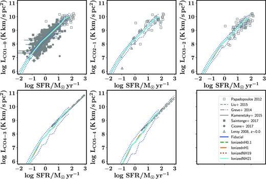
The CO J=1–0 to 5–4 luminosity of galaxies as a function of their SFR at z = 0 for our fiducial model variant, variants where the densities of the diffuse ISM are |$1\, \rm {cm}^{-3}$| (IonizednH1) and |$0.1\, \rm {cm}^{-3}$| (IonizednH0.1), and variants where the column density are 1019 (IonizedNH19) and |$10^{21}\, \rm {cm}^{-2}$| (IonizedNH21), respectively. This figure is similar to Fig. 7. The choice for density of the diffuse atomic ISM has no effect on the predicted CO luminosities of galaxies.
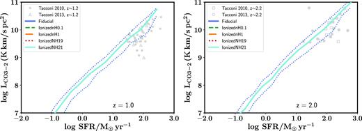
The CO J=3–2 luminosity of galaxies at z = 1 and 2 as a function of their SFR for our fiducial model variant, variants where the densities of the diffuse ISM are |$1\, \rm {cm}^{-3}$| (IonizednH1) and |$0.1\, \rm {cm}^{-3}$| (IonizednH0.1), and variants where the column density are 1019 (IonizedNH19) and |$10^{21}\, \rm {cm}^{-2}$| (IonizedNH21), respectively. This figure is similar to Fig. 8. The choice for density of the diffuse atomic ISM has no effect on the predicted CO luminosities of galaxies.
![The [CI] 1–0 luminosity of galaxies at z = 0 as a function of their SFR for our fiducial model variant, variants where the densities of the diffuse ISM are $1\, \rm {cm}^{-3}$ (IonizednH1) and $0.1\, \rm {cm}^{-3}$ (IonizednH0.1), and variants where the column density are 1019 (IonizedNH19) and $10^{21}\, \rm {cm}^{-2}$ (IonizedNH21), respectively. This figure is similar to Fig. 9. The choice for density of the diffuse atomic ISM has no effect on the predicted [C i] luminosities of galaxies.](https://oup.silverchair-cdn.com/oup/backfile/Content_public/Journal/mnras/482/4/10.1093_mnras_sty2969/1/m_sty2969fige3.jpeg?Expires=1749926986&Signature=M7funKY7pf2qtw84KKjStNlQB9OZrlZuvrquEOHeYEB7xUfHwVtAgT2K-EGD2dLHR0H34fRUeC4TEgdKMUe3ZLM~peJx3nJ3o5Rfq3rLqBIKTCaXcmZ9LAE3y-pbIYMLlVN-Ae7A~VKNBEsJavtZ6TtaAGkOqy7JAkDyRUI-nfZCdWpcwmjzZc9Z7i9mV6d983WNHkSXjp~9Vc1nfHOj7NEL92d8F7tlyXSqf5TROL~EDFCGQAVrxiNKQLj4aivsvJF-7r7ZQ3qwAbfCzCyMGgtyRBS~5FGL49V0MAgxyFgHikv4HCddkLvM5gR1JqDM3PF51NATK2y1wgPaCSgZ5A__&Key-Pair-Id=APKAIE5G5CRDK6RD3PGA)
The [CI] 1–0 luminosity of galaxies at z = 0 as a function of their SFR for our fiducial model variant, variants where the densities of the diffuse ISM are |$1\, \rm {cm}^{-3}$| (IonizednH1) and |$0.1\, \rm {cm}^{-3}$| (IonizednH0.1), and variants where the column density are 1019 (IonizedNH19) and |$10^{21}\, \rm {cm}^{-2}$| (IonizedNH21), respectively. This figure is similar to Fig. 9. The choice for density of the diffuse atomic ISM has no effect on the predicted [C i] luminosities of galaxies.
Author notes
MPIA Fellow.
