


ABSTRACT
We present the dynamical status of the Galactic globular cluster NGC 6656 using the spatial distribution of blue straggler stars (BSSs). A combination of multi-wavelength high-resolution space- and ground-based data are used to cover a large cluster region. We determine the centre of gravity (Cgrav) and construct the projected density profile of the cluster using the probable cluster members selected from the Hubble Space Telescope and Gaia Data Release 2 proper-motion data sets. The projected density profile in the investigated region is nicely reproduced by a single-mass King model, with core (rc) and tidal (rt) radii of 75″.2 ± 3″.1 and 35′.6 ± 1′.1 respectively. In total, 90 BSSs are identified on the basis of proper-motion data in the region of radius 625″. The average mass of the BSSs is determined as 1.06 ± 0.09 M|$\odot$| and with an age range of 0.5 to 7 Gyr. The BSS radial distribution shows a bimodal trend, with a peak in the centre, a minimum at r ∼ rc and a rising tendency in the outer region. The BSS radial distribution shows a flat behaviour in the outermost region of the cluster. We also estimate the |$A^{+}_{r_\mathrm{h}}$| parameter as an alternative indicator of the dynamical status of the cluster; this is found to be 0.038 ± 0.016. Based on the radial distribution and |$A^{+}_{r_\mathrm{h}}$| parameter, we conclude that NGC 6656 is an intermediate dynamical age cluster.
1 INTRODUCTION
Globular clusters (GCs) are some of the oldest systems, where stellar interactions occur due to the high stellar density of the system. These stellar interactions lead to several dynamical processes, such as stellar collisions, core collapse, stellar mergers, two-body relaxation and mass segregation from equipartition of energy (Meylan & Heggie 1997). These dynamical processes result in several exotic populations, like low-mass millisecond pulsars, cataclysmic variables and blue straggler stars (BSSs) (Bailyn 1995; Ferraro et al. 2001). Among these exotic populations, BSSs are found in bulk and therefore play a crucial role in understanding the GC internal dynamics.
BSSs were discovered in 1953 by Sandage in the external regions of the GC M3. Sandage (1953) found that these stars appear as an extension of the main sequence and are hotter and more luminous than the main sequence turn-off (MS-TO) point. The actual nature of these peculiar objects is still not clear. Observational evidence (Shara, Saffer & Livio 1997) has shown that BSSs are more massive (M ∼ 1.2 M|$\odot$|) than average stars in GCs (M ∼ 0.3 M|$\odot$|). Hence, they can be affected by dynamical friction, which segregates the BSSs towards the cluster centre (Ferraro et al. 2006).
The construction of a complete sample of BSSs has always been a challenging task. Because of stellar crowding in the central region and the dominant contribution of the luminous cool and bright giants (e.g. red giant branches, RGBs, and sub-giant branches, SGBs), it is difficult to identify BSSs in optical bands. However, in ultraviolet (UV) bands, RGB stars are among the faint ones, whereas BSSs are the brightest objects to be easily identified in this plane (Paresce et al. 1991). Therefore, with the help of UV observations taken with the Hubble Space Telescope (HST), it has become possible to study BSSs in the central regions of dense clusters.
The selection of BSSs is a difficult task on the basis of only photometric data. After the second Gaia Data Release, Gaia DR2, it has now become possible to separate genuine BSSs from field stars using proper-motion information. This allows the study of BSS radial distribution from the very central region out to the large cluster region using HST and wide-field imagers mounted on ground-based telescopes. Various studies have been done on the distribution of BSSs in the literature. On the basis of the shape of the observed BSS radial distribution, Ferraro et al. (2012) (hereafter F12) grouped GCs into three families.
In Family I, the BSS radial distribution shows a lat distribution, suggesting that dynamical friction has not yet segregated the BSSs located in the innermost cluster region. Various investigations of many GCs, e.g. ω Centauri studied by Ferraro et al. (2006), Palomar 14 by Beccari et al. (2011) and NGC 2419 by Dalessandro et al. (2008b) show flat BSS radial distributions and are classified as Family I clusters.
Several clusters show bimodality in their BSS radial distributions and are classified as Family II clusters. Examples of Family II clusters are M53 (Beccari et al. 2008), NGC 6388 (Dalessandro et al. 2008a), 47 Tuc (Ferraro et al. 2004), M5 (Lanzoni et al. 2007a), M55 (Lanzoni et al. 2007c), NGC 6752 (Sabbi et al. 2004) and NGC 5824 (Sanna et al. 2014). In these clusters bimodality is seen with a peak in the inner region, a clear minimum at rmin and an external rising trend. rmin indicates the distance up to which the role of dynamical friction can be effectively seen.
Family III clusters show a monotonically decreasing radial distribution of BSS, with only a central peak followed by a rapid decline and no signs of an external upturn. Many GCs, e.g. M80 and M30 studied by F12, M79 by Lanzoni et al. (2007b) and M75 by Contreras Ramos et al. (2012), have shown unimodal behaviour in their BSS radial distributions. In these clusters, the dynamical friction has already moved the most distant BSS toward the cluster centre.
As mentioned in F12, these different families correspond to the different dynamical ages of the clusters. Families I, II and III are termed dynamically young, dynamically intermediate and dynamically old clusters respectively.
In this paper, we present the dynamical status of the Galactic GC NGC 6656 (M22) using the radial distribution of the BSS population. NGC 6656 (αJ2000 = 18h36m23|${^{\rm s}_{.}}$|94, δJ2000 = −23°54′17|${^{\prime\prime}_{.}}$|1, Harris 1996 (2010 edition)1 (hereafter HA10) is one of the nearest globular clusters at a distance of 3.2 kpc from the Sun. The core radius of NGC 6656 is ∼1.3 pc and this is a low-density cluster (< 104 M|$\odot$| pc−3). Baldwin et al. (2016) studied the BSS kinematic profile of 19 GCs including NGC 6656 using the HST proper-motion catalogue and they identified 34 BSSs in the central region of NGC 6656. They calculated the average mass of BSSs as |$1.49^{+0.47}_{-0.28}$| M|$\odot$|. The present analysis of the BSS is performed in a larger region (625″ in radius) of the cluster. In addition to this, BSSs are selected from the HST proper-motion catalogue in the central region and the Gaia DR2 catalogue in the outer region of the cluster.
2 DATA SETS AND ANALYSIS
2.1 Data sets
In order to select the BSSs in the entire sample, we need a high-resolution (HR) data set in the central region and a wide-field (WF) data set in the outer region of the cluster. Therefore, we used HST data in the centre and ground-based CCD data taken from the 2.2-m ESO/MPI telescope in the outer region of the cluster.
For the HR data set, we used the astro-photometric catalogue2 provided by Soto et al. (2017). The data sets used in this catalogue are taken from the Hubble Space Telescope UV Legacy Survey of Galactic Globular Clusters (GO-13297) and from two other projects, GO-12311 and GO-12605 (Piotto et al. 2015). The photometric data in this catalogue are in the F275W, F336W and F438W filters, which are taken from Wide Field Camera 3 (WFC3) through the ultraviolet–visible (UVIS) channel. The WFC3/UVIS camera consists two chips, each of 4096 × 2051 pixels with a pixel scale of 0″.0395 pixel−1, and provides a field of view (FOV) of ∼162″ × 162″. This catalogue also provides photometric data in the F606W and F814W filters taken from Advanced Camera for Surveys (ACS)/WFC (GO-10775, PI-Sarajedini). The ACS/WFC camera provides a total FOV of ∼202″ × 202″ with a pixel scale of 0″.05 pixel−1. The respective circular FOV is shown in the upper-right panel of Fig. 1. In addition to the photometric data, the catalogue also contains relative proper-motion information on stars, which is calculated by using the ACS and WFC3 UV positions as the first and second epochs, respectively.
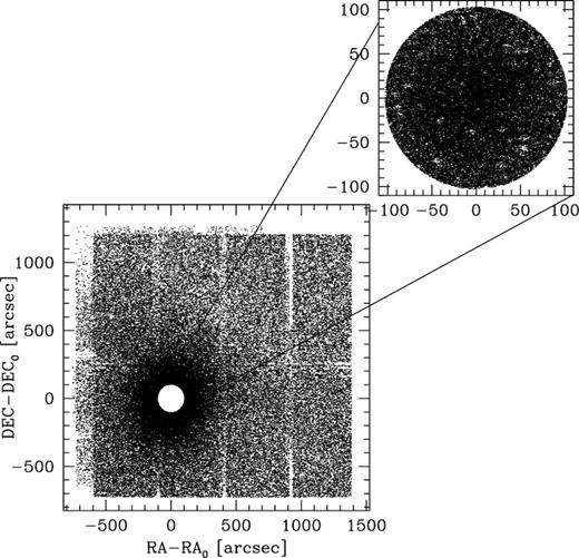
The wide-field data set covering the large cluster region. A map of all the stars found in the WF images is plotted with respect to Cgrav and the open region located towards the cluster centre is taken from the HR sample. A map of the high-resolution data set is shown in the top-right corner of the figure.
For the WF sample, we used archival images3 taken with the Wide-Field Imager (WFI) mounted at the 2.2-m ESO/MPI telescope (La Silla, Chile). A set of wide-field B, V, I and U images was used to sample the BSSs over a larger FOV. The WFI data set in B, V, I was observed on 1999 May 15, and the U data set was observed on 2012 April 20. The aim of selecting the U filter was to fill the gaps between the CCD chips. The WFI consists of eight CCD chips placed together (each composed of 2048 × 4096 pixels, with a pixel scale ∼0″.238 pixel−1), with a total FOV of ∼ 34′ × 33′ as shown in Fig. 1.
2.2 Data reduction and calibration of the 2.2-m ESO data set
The WF images were reduced with the procedures explained in Anderson et al. (2006) (hereafter A06). The pre-processing was done using mscred package under iraf. As mentioned in A06, the shape of the Point Spread Function (PSF) in the WF images varies significantly with the position. Therefore, an array of 9 PSFs per CCD chip (3 × 3) is constructed to minimize the spatial variability down to 1 per cent. The PSFs are constructed from an empirical grid of the size of a quarter pixel. Each PSF is represented by a 201 × 201 grid, centred at (101,101) and extending out to a radius of 25 pixels.
In order to find the instrumental magnitudes and positions from the array of PSFs, an automated code described in A06 is used. The code starts by finding the brightest stars and goes deeper into the fainter stars. Also, to minimize the effect of geometric distortion, the distortion solution derived in A06 is used. However, the geometric distortion solution, particularly for U, is not appropriate for astrometry (A06) and the astrometric solutions can be affected due to systematic errors.
To transform the averaged X, Y coordinates to the corresponding right ascension (αJ2000) and declination (δJ2000) we used the ccmap and cctran tasks available in iraf. An accuracy of ∼0″.1 is obtained in RA and Dec transformation. The U, B, V and I instrumental magnitudes (exposure time and airmass corrected) of the WF images are converted into the F336W, F438W, F606W and F814W VEGAMAG photometric system by using the transformations derived on the basis of about thousand common stars between the HR and WF data sets. Only stars brighter than 20 mag in the F606W filter are used for calibration purposes.
In order to derive the photometric zero-points and colour terms, we used the following transformation equations:
F336Wstd = Uins + Cu * (Uins − Bins) + Zu
F438Wstd = Bins + Cb * (Bins − Vins) + Zb
F606Wstd = Vins + Cv * (Vins − Iins) + Zv
F814Wstd = Iins + Ci * (Vins − Iins) + Zi
where instrumental magnitudes and standard magnitudes are represented by the subscripts ‘ins’ and ‘std’, respectively. In the above equations, Cu, Cb, Cv and Ci denote the colour coefficients, while Zu, Zb, Zv and Zi are the zero-points. The corresponding values of the colour coefficients are 0.37, 0.47, -0.30 and 0.028 and zero-points are 21.09, 24.77, 24.06 and 23.44 mag respectively.
3 FIELD-STAR DECONTAMINATION
The photometric data sets are contaminated by the presence of field stars. The field-star contamination can be reduced by using proper-motion information on the stars. Soto et al. (2017) contains relative proper-motion information for the stars common in the ACS and WFC3 FOV. An analysis of the vector-point diagram (VPD) shown in Soto et al. (2017) exhibits that the stars lying outside the radius 0.35 pixel can be considered as field stars. We have adopted the same criteria as discussed in Soto et al. (2017) for selection of members for the HR sample.
The Gaia DR2 catalogue contains the astrometric and photometric information for all the stars down to G ∼ 21 mag (Gaia Collaboration et al. 2016, 2018). The Gaia DR2 proper-motion data are used to select the members outside the HR sample. A VPD for all the stars except the HR sample is shown in Fig. 2. The stars plotted in the VPD have an accuracy of ≤ 1 mas yr−1 in both proper-motion directions. From the VPD we can see that cluster stars are clearly separated from field stars. The centres of the cluster and field-star distributions are (9.81, -5.57) and (-1.72, -4.35) mas yr−1 respectively. We define the selection criteria for cluster members located within the circle of radius 3.0 mas yr−1 around the centre of cluster distribution as shown in Fig. 2. For further analysis, we used only those stars that are lying within the radius of 3.0 mas yr−1.
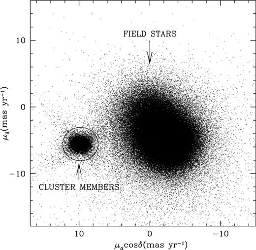
A vector-point diagram (VPD) for the stars with proper-motion information in the Gaia DR2 catalogue. The criterion for selection of cluster members is indicated by a circle of radius 3.0 mas yr−1 around the cluster centre (9.81, -5.57) mas yr−1.
4 RESULTS AND DISCUSSIONS
4.1 Centre of gravity
Stellar evolutionary theories say that stellar luminosities are not directly proportional to stellar masses in a cluster (Montegriffo et al. 1995). The estimation of the geometrical centre (Cgrav) for the cluster may differ significantly from the previously derived centre of luminosity (Clum) values using the surface-brightness distribution. By considering the centre reported in HA10 as an initial guess, the centre of gravity Cgrav is estimated by taking the average of the α and δ of stars for the HR data set. Using the iterative method described in Contreras Ramos et al. (2012), we constructed four circular areas with different radii (10″, 11″, 12″ and 13″) and, for each of these radii, three different magnitude limits (mF606W = 20.5, 21 and 21.5 mag) are consider to reduce the effect of incompleteness. We estimated Cgrav as αJ2000 = 18h36m24|${^{\rm s}_{.}}$|0 and δJ2000 = −23°54′16|${^{\prime\prime}_{.}}$|4 by averaging the values of Cgrav computed over all the 12 different combinations. Our calculated Cgrav value differs by 0|${^{\prime\prime}_{.}}$|5 in α and δ from the value estimated by Goldsbury et al. (2010) using the density contour method.
4.2 Projected density profile
To construct the projected density profile (PDP) of the cluster, we made a catalogue of stars with HST in the centre and Gaia DR2 in the outer region. We considered Gaia DR2 stars because the catalogue is complete up to G = 18 mag (Arenou et al. 2018). We also transformed the HST F606W to the Gaia G-band magnitude using the relation derived in Jordi et al. (2010).
In order to obtain the structural parameters of the cluster, we constructed the PDP of NGC 6656, starting from Cgrav out to ∼36′ (tidal radius). We divided the area into 19 concentric annuli with varying radii centred on Cgrav, and each annulus is divided into four equivalent sub-sectors. The density estimation for each sub-sector is done by counting the stars present in the region divided by the area of the sub-sector. The resulting density for each annulus is estimated by averaging the densities of the sub-sectors and the standard deviation in the average is considered as the uncertainty in the annulus densities. The radius of each annulus is considered as the midpoint value of the corresponding radial bin.
The resultant PDP of NGC 6656 is shown in Fig. 3. The PDP is nicely fitted with an isotropic single-mass King model given by King (1962). The fitting provides the core (rc) and tidal (rt) radii as 75″.2 ± 3″.1 and 35′.6 ± 1′.1 respectively. In HA10 and Kunder et al. (2014), rc and rt are listed as rc ≃ 79″.8 and rt ≃ 31′.9. Trager, King & Djorgovski (1995) have also estimated rc and rt as 85″.1 and 28′.9 respectively, using the surface-brightness profile of the cluster. The present estimates of rc and rt are quite different from the previous studies. However, the current estimates are based on proper-motion data and are considered to be more reliable than the earlier investigations.
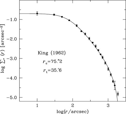
Observed projected density profile, plotted over ∼36′ for the cluster NGC 6656. The density profile is nicely reproduced by an isotropic single-mass King model with the parameters shown in the box. The continuous line shows the King (1962) profile.
4.3 Selection of BSS and reference populations
To study the BSS radial distribution, the first step is to select genuine BSS and reference populations (horizontal branches, HBs, or GBs (RGB + SGB)) carefully. For this purpose, we used the selected cluster members as described in Section 3.
4.3.1 The BSS population
We adopted the UV-CMD (mF275W, mF275W − mF336W) as our primary selection criteria for selecting the BSSs. In this plane, BSSs are easily distinguishable from cooler giants (RGB or asymptotic giant branches, AGBs). As shown in Fig. 4, the BSS populations follow a vertical sequence in the UV-CMD. The contamination from the sub-giant branch and MS-TO is minimized by adopting mF275W = 18.65 mag as the limiting magnitude of the BSS selection box. A total of 26 BSSs are identified in the inner sample (r ≤ 104″), using the UV-CMD. These BSSs are also checked for membership as described in Section 3 and found to be genuine members of the cluster.
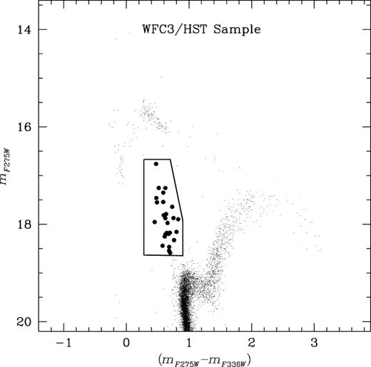
The selection criteria for the BSSs in the UV-CMD (mF275W, mF275W − mF336W) for the HR sample are shown with a box. The selected BSSs are shown with filled dots.
Once selected from the UV-CMD, the BSSs are replotted in the optical-CMD (mF606W, mF606W − mF814W) to define the size of the selection box in the optical band. Based on the position of 26 BSSs in the optical-CMD, we defined the selection-box criteria (15.65 < mF606W < 17.12 and 0.36 < mF606W − mF814W < 0.65) as shown in the left-hand panel of Fig. 5. Six more BSSs in the ACS FOV, not covered by the WFC3 FOV, are identified in the inner sample using the optical-CMD. Based on the member selection norms, they are bona fide members of the cluster. Finally, a total of 32 BSSs are identified in the inner sample. Baldwin et al. (2016) found 34 BSSs in the region of 202 × 202 arcsec2 using the (mF814W, mF606W − mF814W) CMD. The area investigated by Baldwin et al. (2016) is larger than that in the present analysis.
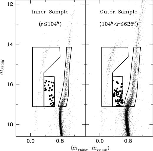
Left: the optical-CMD (mF606W, mF606W − mF814W) of the inner sample (r ≤ 104″). Right: the optical-CMD of the outer sample (104″ < r ≤ 625″). The selection boxes for selecting the BSSs, HBs and GBs are also shown. The BSSs are represented by filled dots.
For the outer sample (104″ < r ≤ 625″), we adopted the same selection box as used for the inner sample, shown in the right-hand panel of Fig. 5. In this way, we found 58 BSSs in the outer sample. Therefore, a total of 90 BSSs are identified from the entire (inner + outer) sample on the basis of photometric and proper-motion data.
4.3.2 The selection of reference populations
In order to carry out a qualitative study of BSSs in terms of radial distribution and specific frequency, the definition of the reference population is very necessary. The reference population should show a non-peculiar radial trend within the cluster. According to Lanzoni et al. (2007c) and Renzini & Fusi Pecci (1988), the number of stars in any post-MS stage is proportional to the duration of the evolutionary phase itself. The specific frequencies (NHB/NGB) are expected to be constant and equal to the ratio between the evolutionary timescales of the HB and GB phases. Therefore, we considered these branches as reference populations. We set the same fainter magnitude limit for BSSs and reference populations so that our selection is not affected by the completeness of the sample. For the selection of the reference population, we used the optical-CMD as shown in Fig. 5. We made a box around the HB population in such a way that it should contain most of the HB stars. In this way a total of 428 (119 in the inner sample and 309 in the outer sample) HB reference stars are identified.
For GB population selection, we defined a mean ridge-line by taking the average in colour (mF606W − mF814W) in the interval of 0.4 mag in mF606W magnitude. For each sample (inner and outer), we used a 3σ selection-box criterion defined from the mean ridge-line. Here, σ is the standard deviation in the mean colour. This is done to reduce the effects of differential reddening and error in photometric calibration. In this way, we found 1233 and 2779 GB reference stars in the inner and outer samples respectively.
Finally, we found 428 HB stars and 4012 GB stars as reference populations in the entire sample.
4.4 The BSS mass distribution
The locations of BSSs in the optical-CMD suggest that they are massive in comparison to normal stars in the GCs. Their masses are estimated by comparing their location in the CMD with theoretical isochrones taken from Girardi et al. (2002). Fig. 6 shows a set of theoretical isochrones fitted to the population of 90 BSSs with an age range of 0.5 to 7 Gyr, in steps of 0.5 Gyr. The metallicity ([Fe/H] = −1.72) and the distance modulus ((m − M)V = 13.60) values of the cluster are adopted from the HA10 catalogue. The projection of the BSSs on the nearest isochrone is used to derive their masses. In this way, BSS masses are estimated in a range of 0.90−1.35 M|$\odot$|. The frequency distribution of BSSs in the different mass intervals is listed in Table 1. It is clear from the table that the maximum number of BSS stars is in the range of 0.95–1.00 M|$\odot$|. The average mass of BSSs is found to be 1.06 ± 0.09 M|$\odot$|.
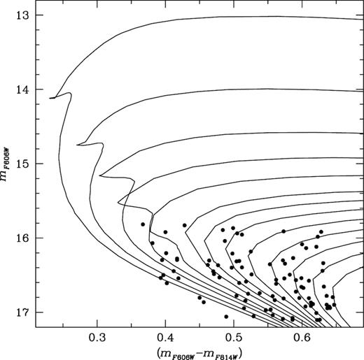
The optical-CMD for 90 BSSs identified in the present analysis. The continuous lines are theoretical isochrones taken from Girardi et al. (2002) and fitted to the BSSs.
The frequency distribution of BSSs in different mass intervals.
| Mass range | Frequency |
|---|---|
| 0.90–0.95 | 3 |
| 0.95–1.00 | 24 |
| 1.00–1.05 | 18 |
| 1.05–1.10 | 14 |
| 1.10–1.15 | 12 |
| 1.15–1.20 | 5 |
| 1.20–1.25 | 9 |
| 1.25–1.30 | 4 |
| 1.30–1.35 | 1 |
| Mass range | Frequency |
|---|---|
| 0.90–0.95 | 3 |
| 0.95–1.00 | 24 |
| 1.00–1.05 | 18 |
| 1.05–1.10 | 14 |
| 1.10–1.15 | 12 |
| 1.15–1.20 | 5 |
| 1.20–1.25 | 9 |
| 1.25–1.30 | 4 |
| 1.30–1.35 | 1 |
Lanzoni et al. (2007b) have obtained the average mass of BSSs as 1.2 M|$\odot$| in the cluster NGC 1904. Baldwin et al. (2016) have provided a BSS kinematic profile for 19 GCs using the ACS/HST sample and estimated the average mass as |$1.49^{+0.47}_{-0.28}$| M|$\odot$| for the BSSs lying near the centre of the cluster NGC 6656. The present estimate of the average mass of BSSs in NGC 6656 is similar to the value derived by previous authors.
4.5 The radial distribution of BSSs, GBs and HBs
In this section, we present the radial distribution of BSS, GB and HB populations. The cumulative radial distributions of BSSs, GBs and HBs are shown with continuous, dashed and dotted lines respectively in Fig. 7. A comparison of the BSS cumulative radial distribution with the GB and HB distributions indicates that BSSs are more centrally concentrated than reference populations. To get a clearer picture of the distributions we performed a Kolmogorov–Smirnov test.4 The probabilities with which the BSSs have a different radial distribution from the HB and GB populations are 98.3 and 99.9 per cent respectively. This shows that the BSS population is extracted from a different parent population to the reference populations.
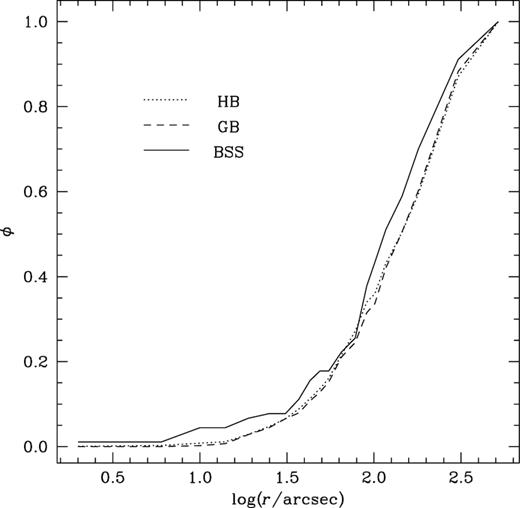
Cumulative radial distribution plot of BSSs (continuous line), HB stars (dotted line) and GB stars (dashed line) with respect to Cgrav of the cluster.
In order to investigate the radial distribution behaviour of BSSs, GBs and HBs further, the cluster region is divided into seven concentric annuli centred on Cgrav. We counted the number of BSS, GB and HB populations in each bin and listed them in Table 2 as NBSS, NGB and NHB. We then computed the specific frequencies |$F^\mathrm{BSS}_\mathrm{GB}$| = NBSS/NGB, |$F^\mathrm{BSS}_\mathrm{HB}$| = NBSS/NHB and |$F^\mathrm{HB}_\mathrm{GB}$| = NHB/NGB. These specific frequencies are plotted with respect to the radius in Fig. 8. The specific frequency |$F^\mathrm{HB}_\mathrm{GB}$| shows a flat behaviour across the entire field of investigation of the cluster. On the other hand, the specific frequencies of BSS show a bimodal trend with both the reference populations. A peak in the centre, a minimum at r ∼ rc and a rising trend in the outer region of the cluster are present. Flattening is also seen in the outermost region of the cluster.
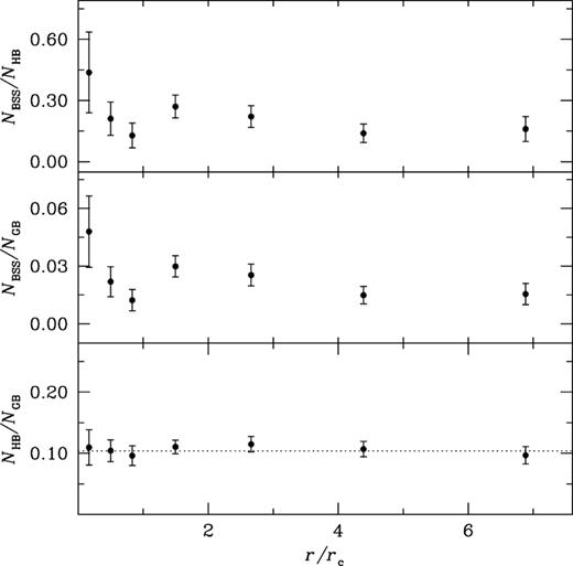
The radial distribution of the specific frequencies |$F^\mathrm{BSS}_\mathrm{HB}$| (top), |$F^\mathrm{BSS}_\mathrm{GB}$| (middle) and |$F^\mathrm{HB}_\mathrm{GB}$| (bottom) plotted with respect to distance from the cluster centre normalized by the core radius. The dotted line shows the mean of all the points plotted in the bottom panel.
The log of the number counts for BSSs and reference populations.
| Radial bin (in arcsec) | NBSS | NHB | NGB | |$L_\mathrm{samp}/L^\mathrm{tot}_\mathrm{samp}$| |
|---|---|---|---|---|
| 0–25 | 7 | 16 | 146 | 0.03 |
| 25–50 | 8 | 38 | 365 | 0.07 |
| 50–75 | 5 | 39 | 406 | 0.09 |
| 75–150 | 30 | 111 | 1005 | 0.24 |
| 150–250 | 21 | 95 | 828 | 0.22 |
| 250–410 | 11 | 79 | 740 | 0.20 |
| 410–625 | 8 | 50 | 517 | 0.14 |
Fig. 9 shows the variation of doubly normalized ratios of BSS (RBSS), HB (RHB) and GB (RGB) populations with the radial distance normalized to rc. The upper panel represents RBSS and RHB, while the lower panel represents RBSS and RGB with respect to r/rc. The value of RBSS show a peak in the centre, a dip at r ∼ rc and an external rising trend followed by flattening on the outskirts of the cluster. The nature of this plot is very similar to Fig. 8. The resulting radial distributions of RGB and RHB follow the cluster luminosity and have almost a constant value (∼1) as expected from the theory of stellar evolution (Renzini & Fusi Pecci 1988).
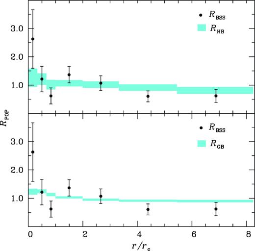
The BSS radial distribution (filled circles) and the reference populations with doubly normalized ratios are plotted with respect to the distance from the cluster centre, normalized to rc. The shaded portion in the upper and lower panels shows the distributions of the HB and GB populations respectively, which is almost constant (∼1). The widths of the shaded regions represent the error bars.
4.5.1 Discussion of the BSS radial distribution
An analysis of Figs 8 and 9 shows that BSS radial distribution in NGC 6656 is bimodal. Dynamical friction plays a very crucial role in shaping the BSS radial distribution. It segregates the massive objects like BSSs that are rotating close to the centre of the cluster. As a result, a peak in the centre and a dip in smaller radii is visible in the BSS radial distribution. The BSSs located on the outskirts of the cluster have not yet been influenced by the action of dynamical friction and hence show a flat distribution. The BSS radial distribution found for NGC 6656 is similar to the previously studied GC M5 (Lanzoni et al. 2007a). The features in the BSS radial distribution can be used as a measure of dynamical age. Based on the shape of the BSS radial distribution, this cluster seems to be an intermediate dynamical age cluster.
4.6 |$A^{+}_{r_\mathrm{h}}$| determination and dynamical status of the cluster
In the previous section, we discussed the dynamical state of the cluster based on the BSS radial distribution in the region of the cluster. Despite several observational confirmations, it has not been possible to reproduce the BSS radial distribution profile from Monte Carlo and N-body simulations of GCs. Also, the bimodality seems to be an unstable and temporary feature (see Miocchi et al. 2015; Hypki & Giersz 2017). Therefore, to reconfirm the dynamical age, we estimated the |$A^{+}_{r_\mathrm{h}}$| parameter proposed by Alessandrini et al. (2016), as a measure of the dynamical status of the cluster. The |$A^{+}_{r_\mathrm{h}}$| parameter is defined as the area between the curves of the cumulative radial distributions of the reference and BSSs populations over the half-mass radius (rh). The value rh = 201″.6 is taken from HA10.
In Fig. 10, we plot the cumulative radial distributions of BSSs and HB in the left-hand panel and BSSs and GB in the right-hand panel. Using these distributions the values of |$A^{+}_{r_\mathrm{h}}$| are estimated as 0.027 and 0.049 for the HB and GB samples respectively. The average value of |$A^{+}_{r_\mathrm{h}}$| = 0.038 ± 0.016. As discussed in L16, |$A^{+}_{r_\mathrm{h}}$| can be adopted as an alternative indicator for measuring the level of dynamical evolution experienced by the cluster from the beginning. They have shown that |$A^{+}_{r_\mathrm{h}}$| can be related to the core relaxation time (trc/tH). Here, tH = 13.7 Gyr is the age of the Universe and trc = 0.34 Gyr is taken from HA10. We plot |$A^{+}_{r_\mathrm{h}}$| versus log(trc/tH) in the lower panel of Fig. 11. The values of |$A^{+}_{r_\mathrm{h}}$| and trc for cluster NGC 6656 are shown with filled circles and the values for other clusters are adopted from L16 and shown with empty circles. As discussed in L16, a decreasing trend of |$A^{+}_{r_\mathrm{h}}$| with relaxation time is seen. It is clear from the plot that the cluster NGC 6656 follows the trend.
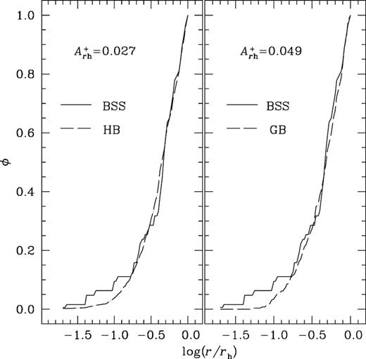
Left: cumulative radial distributions of BSSs and the reference population (HB) plotted over one half-mass radius (rh). Right: cumulative radial distributions of BSSs and GB as the reference population over one rh. The curves of the reference populations are shown with dashed lines and the BSSs are shown with continuous lines.
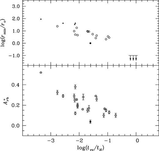
Top|$\colon$| The plot shows the empirical dynamical clock relation defined in F12, as a function of rmin/rc and trc/tH. The open circles show the position of dynamically intermediate clusters and filled triangles the dynamically old clusters. The dynamically young systems are indicated by the lower-limit arrows at rmin = 0.1. The position of NGC 6656 is marked by a filled circle. Bottom|$\colon$| the position of NGC 6656 (filled circle); other clusters are marked by open circles.
In the framework of the empirical dynamical clock relation defined in F12, the position of rmin/rc can be used as an indicator to measure the extent of dynamical evolution of the cluster. Therefore, we plot rmin/rc against trc/tH in the upper panel of Fig. 11. The filled circle represents the cluster NGC 6656. We adopted the values of trc, rmin and rc for other clusters from F12. The filled triangles are dynamically old clusters while open circles are intermediate dynamical age clusters. The dynamically young clusters are plotted as lower-limit arrows at rmin ∼ 0.1. An inspection of this figure reveals that the cluster NGC 6656 lies in the region of intermediate dynamical age clusters. Hence, we suggest that this is an intermediate dynamical age cluster of Family II classification.
Therefore, the BSS radial distribution and |$A^{+}_{r_\mathrm{h}}$| parameter indicates that NGC 6656 is an intermediate dynamical age cluster.
5 SUMMARY AND CONCLUSIONS
In this paper, a combination of multi-wavelength high-resolution space- and ground-based data are used to probe the dynamical status of NGC 6656 based on the BSS radial distribution. The BSS and reference populations are selected from both the photometric and kinematic data. The important findings of the present analysis are the following:
The centre of gravity, Cgrav, of the cluster is determined as αJ2000 = 18h36m24|${^{\rm s}_{.}}$|0 and δJ2000 = −23°54′16|${^{\prime\prime}_{.}}$|4, with an accuracy of ∼0.05″ in both α and δ using the HR data set. The derived PDP can be nicely reproduced by an isotropic single-mass King model and provides rc = 75″.2 ± 3″.1 and rt = 35′.6 ± 1′.1. The stars used for the determination of Cgrav and PDP are selected using proper-motion data.
We identified a total of 90 BSSs in the entire sample, with 32 BSSs lying in the inner sample and 58 BSSs in the outer sample. These BSSs are selected using proper-motion data taken from the HST and Gaia DR2 catalogues. We estimated an average BSS mass of 1.06 ± 0.09 M|$\odot$| and an age range of 0.5 to 7 Gyr.
The BSS radial distribution shows a bimodal trend with a peak in the centre, a minimum at r ∼ rc and an external rising trend followed by flattening in the outermost region of the cluster. We also determined the |$A^{+}_{r_\mathrm{h}}$| parameter, which is found to be 0.038 ± 0.016. This newly determined parameter, along with the bimodal trend in the BSS radial distribution, indicates that this cluster is an intermediate dynamical age cluster. Our results are consistent with the empirical dynamical clock relation defined in F12 and L16, further confirming that NGC 6656 is an intermediate dynamical age cluster belonging to the Family II classification of GCs.
ACKNOWLEDGEMENTS
We thank the anonymous referee for the useful comments that helped us to improve the scientific content of the paper. We would like to acknowledge ESO, for the archival data observed with the ESO Telescope at the La Silla Observatory under program ID 163.O-0741(C) and 088.A-9012(A). This work has made use of data from the European Space Agency (ESA) mission Gaia (https://www.cosmos.esa.int/gaia), processed by the Gaia Data Processing and Analysis Consortium (DPAC, https://www.cosmos.esa.int/web/gaia/dpac/consortium). Funding for the DPAC has been provided by national institutions, in particular, the institutions participating in the Gaia Multilateral Agreement. We are thankful to Dr Andrea Bellini for the description of the astro-photometric catalogue.
