


ABSTRACT
Non-linear bias measurements require a great level of control of potential systematic effects in galaxy redshift surveys. Our goal is to demonstrate the viability of using counts-in-cells (CiC), a statistical measure of the galaxy distribution, as a competitive method to determine linear and higher-order galaxy bias and assess clustering systematics. We measure the galaxy bias by comparing the first four moments of the galaxy density distribution with those of the dark matter distribution. We use data from the MICE simulation to evaluate the performance of this method, and subsequently perform measurements on the public Science Verification data from the Dark Energy Survey. We find that the linear bias obtained with CiC is consistent with measurements of the bias performed using galaxy–galaxy clustering, galaxy–galaxy lensing, cosmic microwave background lensing, and shear |$+$| clustering measurements. Furthermore, we compute the projected (2D) non-linear bias using the expansion |$\delta _{\mathrm{ g}} = \sum _{k=0}^{3} (b_{k}/k!) \delta ^{k}$|, finding a non-zero value for b2 at the 3σ level. We also check a non-local bias model and show that the linear bias measurements are robust to the addition of new parameters. We compare our 2D results to the 3D prediction and find compatibility in the large-scale regime (>30 h−1Mpc).
1 INTRODUCTION
In recent years, photometric redshift galaxy surveys, such as the Sloan Digital Sky Survey (Kollmeier, Zasowski & Rix 2017), the Dark Energy Survey (DES) (Dark Energy Survey Collaboration 2016), and the future Large Synoptic Survey Telescope (Ivezić et al. 2008) and Euclid (Amiaux, Scaramella & Mellier 2012), have arisen as powerful probes of the large-scale structure (LSS) of the Universe and of dark energy. The main advantage of these surveys is their ability to retrieve information from a vast number of objects, yielding unprecedented statistics for different observables in the study of LSS. Their biggest drawback is the lack of line-of-sight precision and the systematic effects associated with it. Thus, well-constrained systematic effects and robust observables are required in order to maximize the performance of such surveys. In this context, simple observables such as the galaxy number counts serve an important role in proving the robustness of a survey. In particular, the galaxy counts-in-cells (CiC), a method that consists of counting the number of galaxies in a given 3D or angular aperture, has been shown to provide valuable information about the LSS (Peebles 1980; Efstathiou et al. 1990; Bernardeau 1994; Gaztañaga 1994; Szapudi 1998) and gives an estimate of how different systematic effects can affect measurements. The CiC can provide insights to higher-order statistical moments of galaxy counts without requiring the computation resources of other methods (Gil-Marín et al. 2015), such as the three- or four-point correlation functions.
Understanding the relation between galaxies and matter (galaxy bias) is essential for the measurement of cosmological parameters (Gaztañaga et al. 2012). The uncertainties in this relation strongly increase the errors in the dark energy equation of state or gravitational growth index (Eriksen & Gaztanaga 2015). Thus, having a wide variety of complementary methods to determine galaxy biasing can help break degeneracies and improve the overall sensitivity for a given galaxy survey.
In this paper we present a method to extract information from the galaxy CiC. Using this method, we measure the projected (angular) galaxy bias (linear and non-linear) in both simulations and observational data from DES, we compare the measured and predicted linear and non-linear bias, and we test for the presence of systematic effects. This data set is ideal for this study since it has been already used for CiC in Clerkin et al. (2017), where it was found that the galaxy density distribution and the weak lensing convergence (κWL) are well described by a lognormal distribution. The main difference between our study and that of Clerkin et al. (2017) is that our main goal is to provide a measurement of the galaxy bias, whereas Clerkin et al. (2017) study convergence maps.
Gruen et al. (2017) also perform CiC in DES data. Combining gravitational lensing information and CiC, they measure the galaxy density probability distribution function (PDF) and obtain cosmological constraints using the redMaGiC-selected galaxies (Rozo et al. 2016) in DES Y1A1 photometric data (Drlica-Wagner et al. 2018). In our case we measure the moments of the galaxy density contrast PDF and compare them to the matter density contrast PDF from simulations (with the same redshift distributions) to study different biasing models, in a different galaxy sample (DES SV).
Throughout the paper, we assume a fiducial flat lambda cold dark matter (ΛCDM) |$+$| ν (one massive neutrino) cosmological model based on Planck 2013 |$+$|WMAP polarization |$+$| ACT/SPT |$+$| BAO, with the parameters (Ade et al. 2014) ωb = 0.0222, ωc = 0.119, ων = 0.00064, h = 0.678, τ = 0.0952, ns = 0.961, and As = 2.21 × 10⁻⁹ at a pivot scale |$\overline{k}=0.05\, \rm {Mpc}^{-1}$| (yielding σ8 = 0.829 at |$z$| = 0), where |$h \equiv H_0 /100\, \rm {km\ s}^{-1}\, \rm {Mpc}^{-1}$| and |$\omega _i\equiv \Omega _i \, h^2$| for each species i.
The paper is organized as follows: In Section 2 we present the data sample used for our analysis. First, we present the simulations used to test and validate the method and afterwards, the data set in which we perform our measurements. In Section 3 we present the CiC theoretical framework and detail our method to obtain the linear and non-linear bias. Sections 4 and 5 present the CiC moments and bias calculations for the MICE simulation and DES SV data set, respectively. In Section 6 we study the systematic uncertainties in our method. Finally, in Section 7, we include some concluding remarks about this work.
2 DATA SAMPLE
2.1 Simulations
In order to test and validate the methodology presented in this paper, we use the MICE simulation (Fosalba et al. 2008; Crocce et al. 2010). MICE is an N-body simulation with cosmological parameters following a flat ΛCDM model with Ωm = 0.25, |$\Omega _\Lambda =0.75$|, Ωb = 0.044, ns = 0.95, and σ8 = 0.8. The simulation covers an octant of the sky, with redshift z between 0 and 1.4, and contains 55 million galaxies in the light-cone. The simulation has a comoving size Lbox = 3072 h−1 Mpc and more than 8 × 10⁹ particles (Crocce et al. 2015). The galaxies in the MICE simulation are selected following the procedure in Crocce et al. (2016), imposing the threshold ievol < 22.5. The MICE simulation has been extensively studied in the literature (Sánchez et al. 2011; Hoffmann, Bel & Gaztanaga 2015; Crocce et al. 2016; Pujol et al. 2017; Garcia-Fernandez et al. 2018), including measurements of the higher-order moments in the dark matter field (Fosalba et al. 2008), providing an ideal validation sample.
2.2 The DES SV benchmark data sample
In this paper we perform measurements of the density contrast distribution and its moments on the DES Science Verification (SV) photometric sample1 (Fig. 1). The DES SV observations were taken using DECam on the Blanco 4 m telescope near La Serena, Chile, covering over 250 deg2 at close to the DES nominal depth. From this sample we make selection cuts in order to recover the LSS benchmark sample (Crocce et al. 2016). By doing this we minimize the possible two-point systematic effects and we ensure completeness. We focus on the SPT-E field, since it is the largest contiguous field and the best analysed, with 60° < RA < 95° and −60° < Dec. < −40° considering only objects with 18 < i < 22.5, where i is MAG_AUTO as measured by SExtractor (Bertin & Arnouts 1996) in the i band. The star–galaxy separation is performed by selecting objects such that WAVG_SPREAD_MODEL > 0.003. The total area considered for our study is then 116.2 deg2 with approximately 2.3 million objects and a number density ng = 5.6 arcmin−2. Several photo-z estimates are available for these data (Sánchez et al. 2014). We will focus on the TPZ (Carrasco Kind & Brunner 2013) and BPZ (Benitez 2000) catalogues. We use the same five redshift bins used in Crocce et al. (2016). We use the redshift distributions from Sánchez et al. (2014), which are depicted in Fig. 2. These distributions have been obtained by comparing the DES SV photometric sample including spectroscopic data from zCOSMOS (Lilly et al. 2007, 2009) and VVDS Deep (Le Fèvre et al. 2013) among other data sets. For more details about the photometric redshift measurement and calibration, we refer the reader to Sánchez et al. (2014).
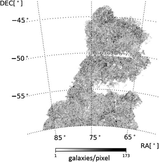
Footprint of the DES SV benchmark sample (Crocce et al. 2016). We use approximately 2.3 million objects contained within this area for our studies.
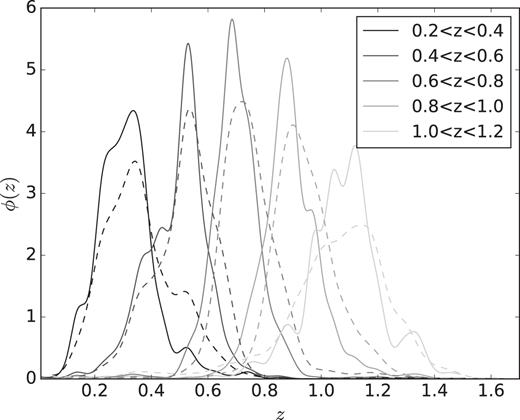
Redshift distribution of the galaxies in each photometric redshift bin using TPZ (solid line) and BPZ (dashed line) in DES SV benchmark data from Crocce et al. (2016). These distributions have been obtained by stacking the photometric redshift PDFs of galaxies in a spectroscopic subsample detailed in Sánchez et al. (2014). Lighter lines represent higher redshift slices.
Several measurements of the linear bias have been performed using this field (Crocce et al. 2016; Giannantonio et al. 2016; Prat et al. 2018), making it ideal for this study.
3 THEORETICAL FRAMEWORK AND METHODOLOGY
3.1 Counts-in-cells
Counts-in-cells (Peebles 1980) is a method used to analyse the LSS based on dividing a galaxy survey into cells of equal volume (Vpix) and counting the number of galaxies in each cell, (Ngal). This method has also been extensively used in the literature to characterize the galaxy distribution (Efstathiou et al. 1990; Bernardeau 1994; Gaztañaga 1994; Szapudi 1998) and, recently, even the neutral hydrogen in simulations (Leicht et al. 2018). In the case of photometric redshift surveys, the lack of precision in the redshift determination makes angular aperture cells more appealing. Numerous examples of the application of CiC using angular aperture cells can be found in the literature (Gaztañaga 1994; Szapudi et al. 2002; Ross, Brunner & Myers 2006; Yang & Saslaw 2011; Wolk et al. 2013).
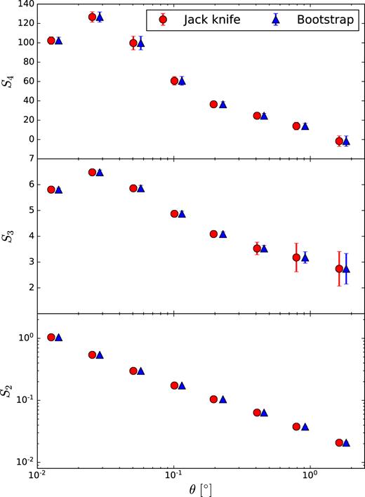
Moments of the density contrast distribution as a function of cell scale in the MICE simulation for the redshift bin 0.2 < |$z$| < 0.4, with jack-knife errors (solid circles) and bootstrap errors (solid triangles). The results for a given scale θ have been separated in the figure for visualization purposes, being the blue triangles, the ones shown at the nominal measured scale.
3.2 Galaxy bias
One of the most important applications of the CiC observable is the determination of the galaxy bias. We observe the galaxy distribution and use it as a proxy to the underlying matter distribution. Both baryons and dark matter structures grow around primordial overdensities via gravitational interaction, so these distributions should be highly correlated. This relationship is called the galaxy bias, which measures how well galaxies trace the dark matter. Galaxy biasing was seen for the first time analysing the clustering of different populations of galaxies (Davis, Geller & Huchra 1978; Dressler 1980). The theoretical relation between galaxy and mass distributions was suggested by Kaiser (1984) and developed by Bardeen et al. (1986). Since then, many different prescriptions have arisen (Fry & Gaztañaga 1993; Bernardeau 1996; Mo & White 1996; Sheth & Tormen 1999; Manera, Sheth & Scoccimarro 2010; M
Bel, Hoffmann & Gaztañaga (2015) point out that ignoring the contribution from the non-local bias can affect the linear and non-linear bias results. As a consequence, we analyse the case when the non-local contribution is included. To do so, we substitute c2 by |$c^{\prime }_{2}=c_{2}-\frac{2}{3}\gamma _{2}$|, where γ2 is the so-called non-local bias parameter (Bel et al. 2015). We will refer to this model as non-local.
Note that we omit the terms higher than third order because, as we will show later, we have very limited sensitivity to b3, and expect to have no sensitivity to b4.
3.3 Estimating the projected linear and non-linear bias
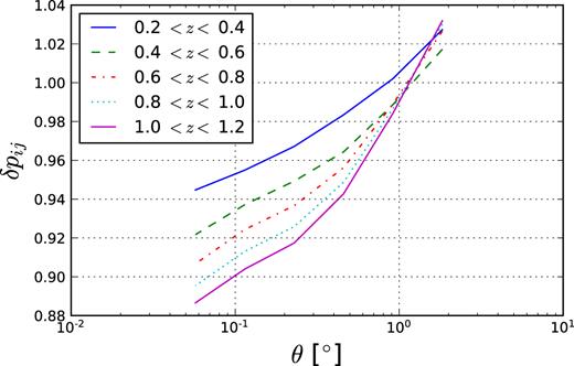
Ratio between S2,m for Ωm = 0.2 (the minimum allowed by Planck priors) and S2,m for our fiducial model as a function of the cell aperture angle θ. The different lines represent different redshift bins. We see that the variation is within 12 per cent of the linear prediction.
We use the following flat priors:
0 < b < 10.
−10 < b2 < 10.
−10 < b3 < 10.
γ2 = 0 (or in the case of the non-local model −10 < γ2 < 10).
These priors have been chosen to prevent unphysical results. We evaluate the likelihood and obtain the best-fitting values and their uncertainties by performing a Markov chain Monte Carlo (MCMC) using the software package emcee (Foreman-Mackey et al. 2013). Summarizing, the method works as follows:
Measure CiC moments using HEALPix pixels in the galaxy sample.
Measure CiC moments using the same pixels and selection function in a dark matter simulation with comparable cosmological parameters.
Evaluate the statistical and systematic uncertainties in the measured moments.
Obtain the best-fitting b, b2, and b3 (and γ2 in the non-local model) using MCMC with the models from equations (8–10).
In summary, in the local model we fit three free parameters, whereas in the non-local model we fit four.
4 RESULTS IN SIMULATIONS
In order to validate this method, we first compute the CiC moments in the MICE simulation (in both galaxies and DM) using a Gaussian selection function ϕ(|$z$|) with σ|$z$| = 0.05(1 |$+$||$z$|). This σ|$z$| is similar to the photometric redshifts found in the data using TPZ (Carrasco Kind & Brunner ) and BPZ (Benitez 2000). We split our sample into five photometric redshift bins: |$z$| ∈ [0.2, 0.4], [0.4, 0.6], [0.6, 0.8], [0.8, 1.0], [1.0, 1.2], mirroring the choice in Crocce et al. (2016). Then we do the same with the SV data sample presented in Section 2.2 with TPZ photometric redshifts.
4.1 Angular moments for MICE
Fig. 5 shows the moments of the density contrast distribution as a function of the cell scale for the different photometric redshift bins. We observe that the moments follow the expected trend; that is, lower redshift bins have higher values for the higher-order moments since non-linear gravitational collapse has a larger effect on these. This is true for all measurements except for the last two redshift bins of the variance S2. This can be due to the magnitude cuts, since the galaxy populations are different at different redshifts. We also see that the larger the cell scale, the smaller the variance S2, since larger cell scales should be more homogeneous. The skewness and kurtosis at linear scales (θ > 0.1°) are constant and of the same order of magnitude as the expected values (S3 ≈ 34/7, S4 ≈ 60 712/1323) (Bernardeau 1994). The behaviour at non-linear scales is due to the non-linearities of the MICE simulation.
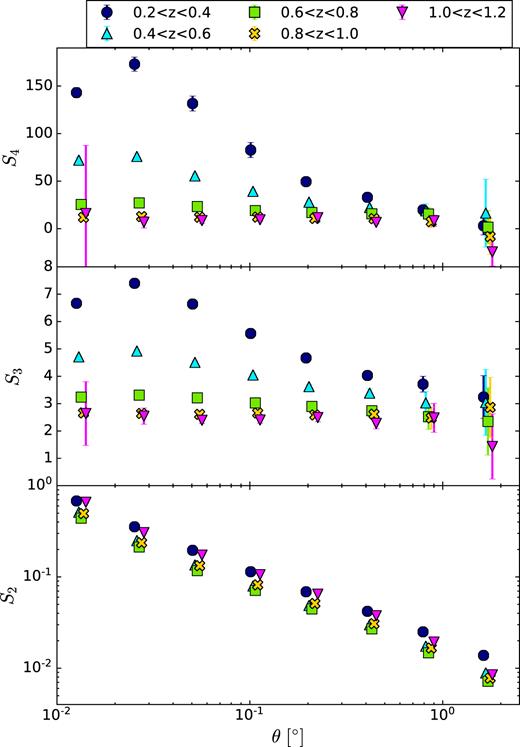
Moments of the density contrast distribution as a function of cell scale in the MICE simulation with Gaussian photometric redshift (Δ|$z$| = 0.2σ|$z$| = 0.05(1 |$+$||$z$|)) for different redshift bins. The results for a given scale θ have been separated in the figure for visualization purposes.
4.2 Projected galaxy bias in MICE simulation
We smear the true redshift with the proper selection function in the MICE dark matter field, obtained from a dilution of the dark matter particles (taking 1/700 of the particles). Chang et al. (2016) demonstrate that the dilution of the dark matter field does not impact their statistics and using the measured moments from the previous section we proceed to perform a simultaneous fit for b, b2, and b3 using the local, non-linear bias model from equations (11)–(13). The fit results are summarized in Fig. 6. We can see the impact of changing the range of θ considered in the fit. In this case we see that including scales smaller than 0.1°, where non-linear clustering has a large impact, affects the b2 results. This, together with the fact that the reduced χ2 minimum value doubles when including θ = 0.05°, clearly shows that we should not consider scales smaller than θ = 0.1°. We can see as well that b3 is compatible with zero and that we have a limited sensitivity to it, given the area used. Thus, the choice of ignoring terms of orders higher than b3 becomes a good approximation. However, for b2 we are able to measure a significant non-zero contribution. We can also see that the predicted values for the 3D non-linear bias parameter b2 are not in good agreement at small scales, while there is an indication of better agreement at larger scales. This suggests that the 2D and 3D values for b2 might be compatible at larger scales, in agreement with Manera & Gaztañaga (2011), who show that the local bias is consistent for scales larger than R > 30–60 h−1 Mpc. They also show that the values of b1 and b2 vary with the scale and converge to a constant value around R > 30–60 h−1 Mpc, which means that the values that we measure here have not yet fully converged. The prediction for b3 seems to be compatible with the estimated values given the size of the error bars. These results show that we should consider b2 as a first-order (small) correction to the linear bias model at these scales for projected (angular) measurements. The individual fits can be seen in Appendix C.
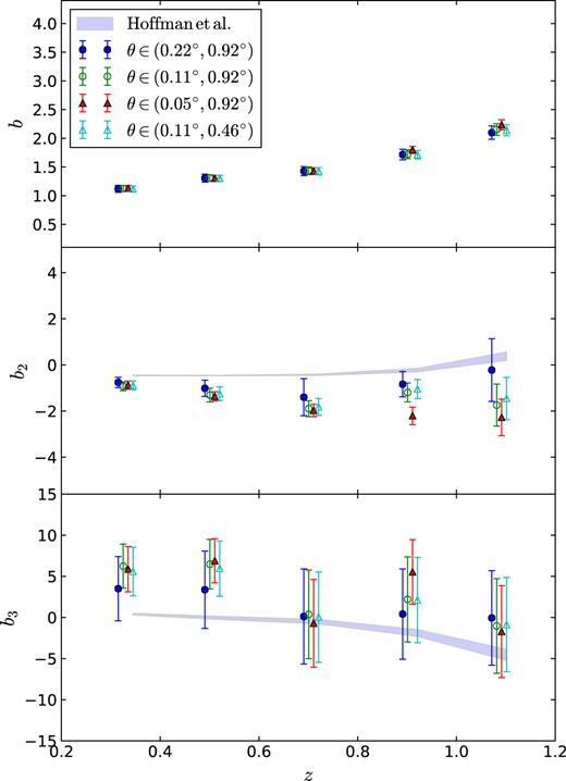
Linear and non-linear bias results as a function of redshift for MICE data with Gaussian photo-z. The different marker shapes represent the best-fitting results considering different ranges of the aperture angle θ. For the solid triangles we consider the range from 0.05° to 0.92°, the open circles are our fiducial case with 0.11° < θ < 0.92°, for the solid circles, we take out the smallest scale in our fiducial case, and in the open triangles we take out the largest scale. The top panel shows the projected linear bias b as a function of redshift, the middle panel shows the best-fitting results for the projected b2, and the lower panel shows b3. The shaded region corresponds to the 3D predicted values using equation (17). The results for a given redshift |$z$| have been separated in the figure for visualization purposes.
4.3 Verification and biasing model comparison
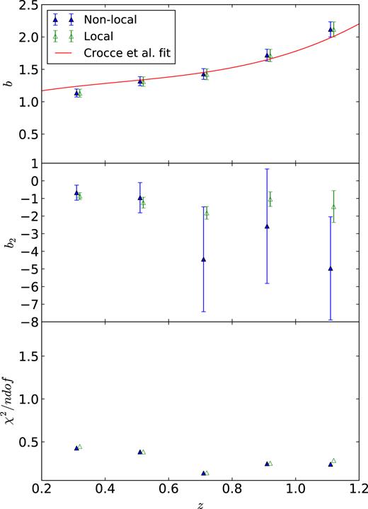
(Top) Comparison between the MICE simulation bias obtained using CiC with different biasing models: non-local (solid triangles) and local (open triangles). We also show the best fit from Crocce et al. (2016; figure 17) as reference. The middle panel shows the equivalent results for b2. This is done for Gaussian photo-z with σ|$z$| = 0.05(1 |$+$||$z$|). (Bottom) Total reduced chi-square for each of the models when fitting the moments to obtain the bias.
5 RESULTS IN DES SV DATA
5.1 Angular moments for DES SV
Using the same footprint, selection cuts, and redshift bins as in Crocce et al. (2016), we compute the moments of the density contrast distribution for the SV data. These results are depicted in Fig. 8 as a function of cell scale for different redshift bins. Here, as in the case of MICE, the variance decreases with the scale. The skewness and kurtosis are also constant and of the same order of magnitude as the theoretical values within errors. The largest differences when compared with the simulation are in the non-linear regime due to the different way in which non-linearities are induced in the simulation and in real data. We also compare to the results from Canada-France-Hawaii Telescope Legacy Survey (CFHTLS) found in Wolk et al. (2013). We find a similar general behaviour as well as the same order of magnitude in the measured S3 and S4. However, we do not expect the same exact results since the redshift distributions from CFHTLS do not match exactly the corresponding distributions in the DES SV data.

Moments of the density contrast distribution of the DES SV benchmark sample as a function of cell scale, for five different redshift bins and different scales. The results for a given scale θ have been separated in the figure for visualization purposes. We compare with the results from Wolk et al. (2013) for CFHTLS marked with solid lines of different colours for the different redshift bins: navy (0.2 < |$z$| < 0.4), cyan (0.4 < |$z$| < 0.6), lime (0.6 < |$z$| < 0.8), yellow (0.8 < |$z$| < 1.0).
5.2 Projected galaxy bias in DES SV
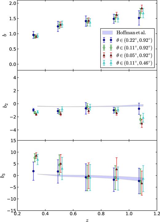
Linear and non-linear bias results as a function of redshift for DES SV data. Systematic uncertainties from Section 6 are already included in these results, excluding the uncertainties associated with the modelling. The different marker shapes represent the best-fitting results considering different ranges of aperture angle θ. For the solid triangles we consider the range from 0.05° to 0.92°, open circles symbolize our fiducial case with 0.11° < θ < 0.92°, in solid circles, we take out the smallest scale in our fiducial case, and in open triangles we take out the largest scale. The shadowed region corresponds to the 3D predicted values using equation (17). The top panel shows the projected linear bias b as a function of redshift, the middle panel shows the best-fitting results for the projected b2, the lower panel shows b3. The results for a given redshift |$z$| have been separated in the figure for visualization purposes.
We also check the measurement of linear bias obtained in this work and compare it with previous measurements on the same data set in Fig. 10. The measurements are generally in good agreement with each other, showing the robustness of the method.
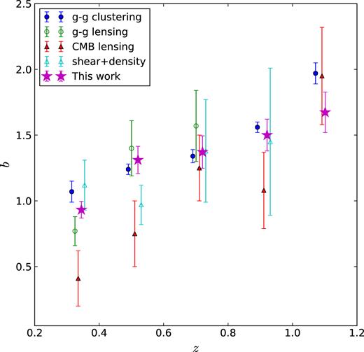
Bias obtained from second-order CiC, including systematic uncertainties from Section 6, compared with the two-point correlation study (Crocce et al. 2016), the CMB–galaxy cross-correlation study (Giannantonio et al. 2016), galaxy–galaxy lensing (Prat et al. 2018), and the shear |$+$| density analysis (Chang et al. 2016). The points for the same |$z$| have been separated in the horizontal axis for visualization purposes.
Future DES data will have a considerably larger area and, as previous MICE measurements show, these measurements will improve. Here we also use the skewness and kurtosis of dark matter from the MICE dark matter simulation, as these quantities hardly depend on the cosmology (Bouchet et al. 1992). We also find that our results are similar to those in Ross et al. (2006). We do not expect them to be equal as the samples are different and the bias depends strongly on the population sample.
6 SYSTEMATIC ERRORS
In this section, we explore the effects that several potential sources of systematic uncertainty have on our moment measurements. Since our main observable is related to the number of galaxy counts in a given redshift interval, we are interested in observational effects that can affect this number. The main potential sources of systematic uncertainties are changes in airmass, seeing, sky brightness, star–galaxy separation, galactic extinction, and possible errors in the determination of the photometric redshift. In order to evaluate their effects, we use the maps introduced in Leistedt et al. (2016). To account for the stellar abundance in our field we proceed as in Crocce et al. (2016) and use the USNO-B1 catalogue (Monet et al. 2003). We also use the dust maps from Schlegel, Finkbeiner & Davis 1998. What follows is a detailed step-by-step guide to our systematic analysis: We select one of the aforementioned maps and locate the pixels where the value of the systematic is below the percentile level t. We compute the moments of the density contrast distribution in these pixels and their respective errors using bootstrapping. We change the threshold to t|$+$| 5, repeat the process, and evaluate the difference between the moments calculated using this threshold divided by the moments in the original footprint ΔSi(t)/〈Si〉. An example of the results of this procedure can be found in Fig. 11. Note that the plot showing the variation of the moments with USNOB shows less points in the horizontal axis. Due to the discrete nature of the map of stellar counts, the 50th and 60th percentiles of the δ distribution of the stellar counts are the same; in order to avoid these problems, we make less bins in this case.
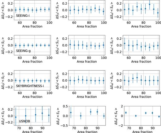
Dependence of the moments Si with the variation in the value of potential systematic effects. We show an example for Nside = 2048 in the redshift bin 0.2 < |$z$| < 0.4 using TPZ. The left column shows the behaviour for S2, the middle column shows S3, and the last column shows the results for S4. The first row corresponds to the results for the seeing in the i band, the second row shows the results for the seeing in the g band, the third row shows the sky brightness in the i band. Finally the last row shows the evolution of the moments with the variation in the number of stars per pixel.
We consider that a systematic effect is present if the average of ΔSi(t)/〈Si〉 is different from zero at a 2σ confidence level or above for the different values of t from the 50th percentile to the 100th percentile. Then, we assign a systematic uncertainty equal to the value of this average. To be conservative, we consider these effects as independent, so we add them in quadrature. We summarize the main systematic effects observed in each redshift bin of our sample.
Bin 0.2 < |$z$| < 0.4:
Seeing in i band: We assign a 3 per cent systematic uncertainty in S4.
Seeing in z band: We assign a 2.5 per cent systematic uncertainty in S4.
Sky brightness r band: We assign a 1 per cent systematic uncertainty in S4.
Sky brightness i band: We assign a 1 per cent systematic uncertainty in S4.
Airmass in g band: We assign a 1 per cent uncertainty in S4.
Airmass in r band: We assign a 1 per cent uncertainty in S4.
Airmass in i band: We assign a 1 per cent uncertainty in S4.
USNO-B stars: We assign a 4 per cent uncertainty to S2, 7 per cent uncertainty to S3, and 9 per cent to S4.
Bin 0.4 < |$z$| < 0.6:
Seeing in z band: We assign a 1.5 per cent uncertainty to S4.
USNO-B stars: We assign a 4 per cent uncertainty to S2, 3 per cent uncertainty to S3, and 4 per cent uncertainty to S4.
Bin 0.6 < |$z$| < 0.8:
Seeing in g band: We assign a 2 per cent uncertainty to S4.
Seeing in r band: We assign a 2 per cent uncertainty to S4.
Sky brightness i band: We assign a 1.5 per cent uncertainty to S3 and 3 per cent systematic uncertainty to S4.
Airmass in g band: We assign a 2.5 per cent uncertainty to S4.
Airmass in r band: We assign a 2 per cent uncertainty to S4.
Airmass in z band: We assign a 1.5 per cent uncertainty to S3 and 3 per cent uncertainty to S4.
USNO-B stars: We assign a 3 per cent uncertainty to S3 and 5 per cent uncertainty to S4.
Bin 0.8 < |$z$| < 1.0:
Seeing in g band: We assign a 2 per cent uncertainty to S4.
Sky brightness in i band: We assign a 2 per cent uncertainty to S3 and a 3.5 per cent uncertainty to S4.
Airmass in g band: We assign a 2 per cent uncertainty to S4.
Airmass in r band: We assign a 3 per cent uncertainty to S4.
USNO-B stars: We assign a 3 per cent uncertainty to S4.
Bin 1.0 < |$z$| < 1.2:
The measurement of S4 in this bin is dominated by systematics.
Sky brightness in i band: We assign 2 per cent to S3.
Sky brightness z band: We assign 3 per cent to S3.
USNO-B stars: We assign a 4.5 per cent uncertainty to S3.
The estimated systematic errors for the bias are propagated from the estimation of the systematics in S2, S3, and S4. Their behaviour is compatible with the systematics found in Crocce et al. (2016). We use the same data masking, excluding regions with large systematic values to recover |$w$|(θ). The linear bias is more robust using CiC since the variance, S2, is less affected by the small-scale power induced by the systematics given that these scales are smoothed out. On the other hand, the non-linear bias is more sensitive to the presence of systematics because they can induce asymmetries in the density contrast distribution.
6.1 Photometric redshift
Photometric redshift is one of the main potential sources of systematic effects in photometric surveys like DES. We have repeated the analysis in DES SV data for a second estimate of the photometric redshift using BPZ (Benitez 2000). In Fig. 12 we compare the results for the two photometric redshift codes and we see that they are in good agreement. The linear bias seems to be the most affected by the choice of a photometric redshift estimator but the results do not show any potential systematic biases. For the non-linear bias we get remarkably consistent results, showing the robustness of this method.
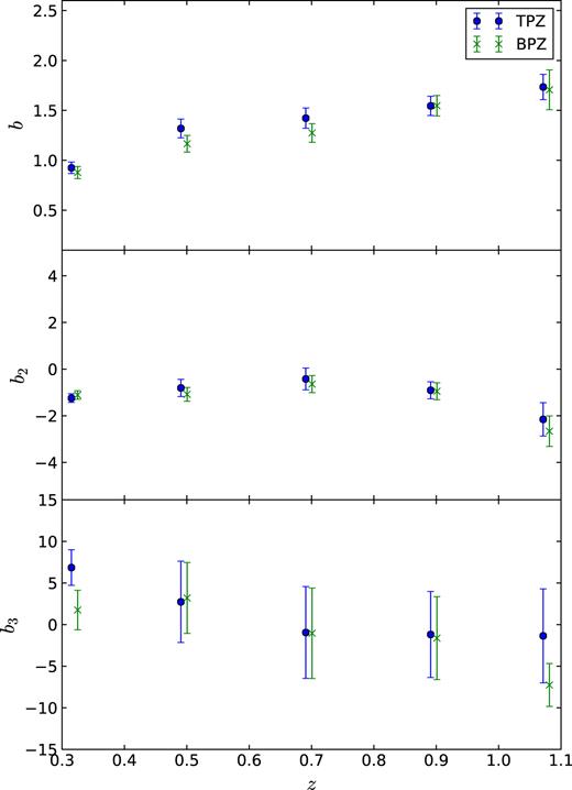
Bias obtained in the SV data from second-order CiC for TPZ (solid blue circles) and BPZ (green crosses). The results for a given redshift |$z$| have been separated in the figure for visualization purposes.
6.2 Biasing models
Apart from the terms that we considered in our model, Bel et al. (2015) found that non-local bias terms are responsible for the overestimation of the linear bias from the three-point correlation in Pollack, Smith & Porciani (2014), Hoffmann et al. (2015), and Manera & Gaztañaga (2011) but that they should not significantly affect second-order statistics. As we mentioned previously in Section 5, we do not expect these terms to have a significant impact on our estimations because we analyse projected quantities over considerable volumes (note that we integrate in the cell and in the redshift slice). Having said that, we test the local and non-local models and find the results depicted in Fig. 13. We can see, as in the case of the simulation, that both models are consistent within errors. This means that choosing the local model does not introduce any systematic uncertainties in our linear bias measurements. However, it affects the b2 measurements and their uncertainty since the new parameters introduced with these more complicated models are correlated with them. We check the probability of b2 being zero for the different models and obtain the results in Table 1. We find b2 to be different from zero at a 3σ level in the worst case (non-local). We also can see that in the first bin, none of the models fit the data well, which is not surprising, given that the range of (comoving) scales is very small (∼1−20 h−1 Mpc) and non-linear clustering dominates.
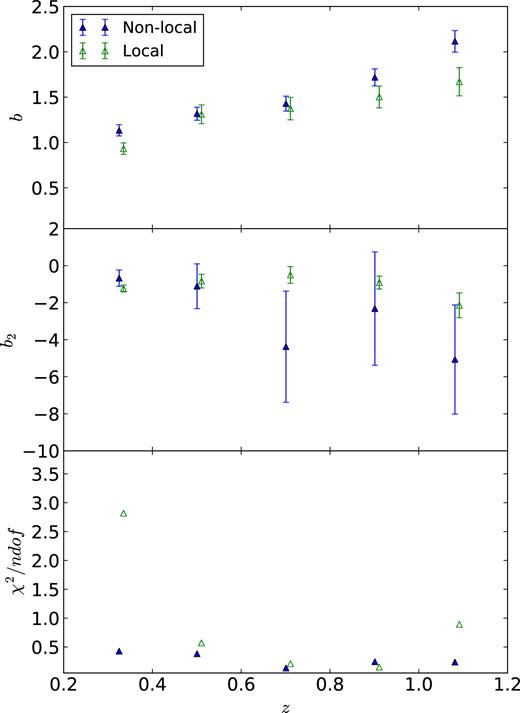
(Top) Comparison between the linear bias results obtained with CiC for SV using different biasing models: non-local (solid triangles) and local (open triangles) using the TPZ sample. (Middle) Comparison between b2 results for the same models as above. (Bottom) Total reduced chi-square for each of the models.
Comparison of the null hypothesis for b2 in DES SV data for the different bias models considered in this work.
| Bias model | χ2 | p-value | ndof |
|---|---|---|---|
| Local | 64.75 | 3 × 10⁻¹³ | 4 |
| Non-local | 12.63 | 0.013 | 4 |
| Bias model | χ2 | p-value | ndof |
|---|---|---|---|
| Local | 64.75 | 3 × 10⁻¹³ | 4 |
| Non-local | 12.63 | 0.013 | 4 |
Finally, we are not considering stochastic models and we are assuming a Poisson shot-noise. This means that our measured b2 could be entangled with stochasticity (Pen 1998; Sato & Matsubara 2013). We leave the study of stochasticity to future works.
6.3 Value of σ8
As mentioned in previous sections, our bias estimation depends linearly on the value of σ8. Thus, if the actual value of σ8 is different from our assumed fiducial value, our results will be biased, and we have to correct for the difference using equation 11. This is why we introduce a systematic uncertainty of |$1.4{{\ \rm per\ cent}}$| (the uncertainty level in σ8 from Ade et al. 2014) which we add in quadrature to the statistical errors in the final estimation of the bias.
7 CONCLUSIONS
CiC is a simple but effective method to obtain the linear and non-linear bias. A good measurement of the galaxy bias is essential to maximize the performance of photometric redshift surveys because it can introduce a systematic effect on the determination of cosmological parameters. The galaxy bias is highly degenerate with other cosmological parameters and an independent method to determine it can break these degeneracies and improve the overall sensitivity to the underlying cosmology. In this paper we have developed a method to extract the bias from CiC. We use the MICE simulation to test our method and then perform measurements on the public Science Verification data from the Dark Energy Survey. The strength of this method is that it is based on a simple observable, the galaxy number counts, and is not demanding computationally.
We check that our linear bias measurement from CiC agrees with the real bias in the MICE simulation. Fig. 7 shows an agreement between our measurement and the one obtained using the angular two-point correlation function. We then obtain the linear bias in the SV data and find that it is in agreement with previous bias measurements from other DES analyses. In Fig. 10, we see that the CiC values are compatible with the two-point correlation study (Crocce et al. 2016), the CMB–galaxy cross-correlation study (Giannantonio et al. 2016), and the galaxy–galaxy lensing (Prat et al. 2018), and we demonstrate that these results are robust to the addition of new parameters in the biasing model, such as the non-local bias. Finally, we compute the non-linear bias parameters up to third order. We detect a significant non-zero b2 component. It appears that the 2D and 3D predictions of the non-linear bias are in better agreement at larger scales, as expected. However, given the uncertainties associated with these quantities, it is difficult to draw any conclusions from b3 despite its compatibility with the expected 3D prediction. When more data is available, we plan to check if we can improve our constraints on b3 and whether the agreement with the 3D prediction improves as well. The systematic errors are in general lower than the statistical errors, in agreement with the systematic study done by Crocce et al. (2016).
ACKNOWLEDGEMENTS
We would like to thank Jonathan Loveday for carefully reading the manuscript and providing invaluable feedback that improved the overall quality of this work. We thank Anna M. Porredon for providing theoretical correlation functions for checking purposes and Cora Uhlemann for her insightful comments.
We acknowledge the use of data from the MICE simulations, publicly available at http://www.ice.cat/mice. We also acknowledge the use of scipy, numpy,astropy, healpy, emcee, and ipython for this work. FJS acknowledges support from the U.S. Department of Energy. Funding for the DES projects has been provided by the U.S. Department of Energy, the U.S. National Science Foundation, the Ministry of Science and Education of Spain, the Science and Technology Facilities Council of the United Kingdom, the Higher Education Funding Council for England, the National Center for Supercomputing Applications at the University of Illinois at Urbana-Champaign, the Kavli Institute of Cosmological Physics at the University of Chicago, the Center for Cosmology and Astro-Particle Physics at the Ohio State University, the Mitchell Institute for Fundamental Physics and Astronomy at Texas A&M University, Financiadora de Estudos e Projetos, Fundação Carlos Chagas Filho de Amparo à Pesquisa do Estado do Rio de Janeiro, Conselho Nacional de Desenvolvimento Científico e Tecnológico, and the Ministério da Ciência, Tecnologia e Inovação, the Deutsche Forschungsgemeinschaft, and the Collaborating Institutions in the Dark Energy Survey.
The Collaborating Institutions are Argonne National Laboratory, the University of California at Santa Cruz, the University of Cambridge, Centro de Investigaciones Energéticas, Medioambientales y Tecnológicas-Madrid, the University of Chicago, University College London, the DES-Brazil Consortium, the University of Edinburgh, the Eidgenössische Technische Hochschule (ETH) Zürich, Fermi National Accelerator Laboratory, the University of Illinois at Urbana-Champaign, the Institut de Ciències de l’Espai (IEEC/CSIC), the Institut de Física d’Altes Energies, Lawrence Berkeley National Laboratory, the Ludwig-Maximilians Universität München and the associated Excellence Cluster Universe, the University of Michigan, the National Optical Astronomy Observatory, the University of Nottingham, the Ohio State University, the University of Pennsylvania, the University of Portsmouth, SLAC National Accelerator Laboratory, Stanford University, the University of Sussex, Texas A&M University, and the OzDES Membership Consortium.
Based in part on observations at Cerro Tololo Inter-American Observatory, National Optical Astronomy Observatory, which is operated by the Association of Universities for Research in Astronomy (AURA) under a cooperative agreement with the National Science Foundation.
The DES data management system is supported by the National Science Foundation under grant numbers AST-1138766 and AST-1536171. The DES participants from Spanish institutions are partially supported by MINECO under grants AYA2015-71825, ESP2015-66861, FPA2015-68048, SEV-2016-0588, SEV-2016-0597, and MDM-2015-0509, some of which include ERDF funds from the European Union. The IFAE is partially funded by the CERCA program of the Generalitat de Catalunya. Research leading to these results has received funding from the European Research Council under the European Union’s Seventh Framework Programme (FP7/2007-2013) including ERC grant agreements 240672,291329, and 306478. We acknowledge support from the Australian Research Council Centre of Excellence for All-sky Astrophysics (CAASTRO), through project number CE110001020, and the Brazilian Instituto Nacional de Ciência e Tecnologia (INCT) e-Universe (CNPq grant 465376/2014-2).
This manuscript has been authored by Fermi Research Alliance, LLC under Contract No. DE-AC02-07CH11359 with the U.S. Department of Energy, Office of Science, Office of High Energy Physics. The United States Government retains and the publisher, by accepting the article for publication, acknowledges that the United States Government retains a non-exclusive, paid-up, irrevocable, worldwide license to publish or reproduce the published form of this manuscript, or allow others to do so, for United States Government purposes.
We are grateful for the extraordinary contributions of our CTIO colleagues and the DECam Construction, Commissioning, and Science Verification teams in achieving the excellent instrument and telescope conditions that have made this work possible. The success of this project also relies critically on the expertise and dedication of the DES Data Management group.
Footnotes
This sample is available at https://des.ncsa.illinois.edu/releases/sva1.
REFERENCES
APPENDIX A: DIFFERENT PIXEL SHAPES
We check with the MICE simulation in a thin redshift bin (0.95 < |$z$| < 1.05) that as long as we have regular polygon pixels the difference in the moments of the density contrast is negligible. In Fig. A1 we see that the difference is negligible for the more symmetrical pixels and higher for less symmetrical ones. The angular aperture, θ, is estimated as the square root of the pixel area. We compare rectangular pixels with HEALpix pixels. We divide the sphere into rectangular pixels taking nra parts in right ascension and nct parts in sin dec where the number of pixels is npix = nra × nct = 12(Nside × Nside). We have taken six different pixel shapes numbered from 1 to 6. Pixels number 3 (nra = 3Nside, nct = 4Nside), 4 (nra = 4Nside, nct = 3Nside), and 6 (nra = 6Nside, nct = 2Nside) are close to being squares, but pixels number 1 (nra = 12Nside, nct = 1Nside), 2 (nra = 1Nside, nct = 12Nside), and 5 (nra = 2Nside, nct = 6Nside) are far from being regular polygons. When we compare square and HEALpix pixels, we see that the measured moments are in perfect agreement.
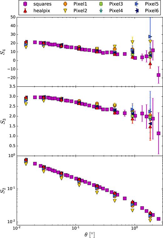
Moments of the density contrast distribution as a function of the cell scale using data from MICE in the redshift slice 0.95 < |$z$| < 1.05 for different pixel shapes. Pixels number 3 (nra = 3Nside, nct = 4Nside), 4 (nra = 4Nside, nct = 3Nside), and 6 (nra = 6Nside, nct = 2Nside) are close to being squares, but pixels number 1 (nra = 12Nside, nct = 1Nside), 2 (nra = 1Nside, nct = 12Nside), and 5 (nra = 2Nside, nct = 6Nside) are far from being regular polygons.
APPENDIX B: BOUNDARY EFFECTS
To deal with the boundary effects of an irregularly shaped area, we use the mask and degrade its resolution to match each of the pixel scales being used. However, degrading the mask (or increasing the scale) results in an increasing number of partially filled pixels. Only a fraction rA = Afilled/Apixel remain completely inside the footprint. This means that if we assign the same scale to all the pixels of a given Nside value, some pixels will be effectively mapping a different scale. To solve this problem we can either require a minimum fraction of the pixel to be full, rA ≥ X, or compute the fraction of full pixels and perform CiC for that scale. We prefer to use the former because we consider that the scales where we perform the study appropriately map the variations of the density field in which we are interested. This approach also helps to avoid certain boundary effects. For small pixel sizes (similar to the size in the mask), given the large number of pixels, we can safely choose rA = 1. For bigger pixels we try to find a compromise between the amount of area that we lose and the boundary effects. In Figs B1 and B2 we show the area loss using data from MICE in the redshift bin 0.95 < |$z$| < 1.05 with the SV mask for different thresholds in rA and in Fig. B3 the change in the moments for these different area cuts. We see that if we choose pixels that are completely contained inside the mask (rA = 1.0), we lose a lot of area for smaller values of Nside; however, very little area is lost for large values of Nside. It can be seen that results are consistent for the different threshold values for rA. We also see that if we take all the pixels (rA ≥ 0), the difference in the moments is considerable in some cases, and we cannot take just all the pixels inside the mask (rA = 1) because we run out of them for large scales. We set a threshold rA ≥ 0.9 to ensure that the pixels are almost completely embedded in the footprint. This prevents us from mixing scales even for the largest pixel sizes. This can be noted in Fig. B1 where a large drop in area occurs between rA = 0.8 and rA = 0.9 for Nside ≤ 1024, setting this threshold naturally. For most scales this threshold does not change the errors. By choosing rA ≥ 0.9 the effective cell sizes are well determined and the errors are reasonably small.
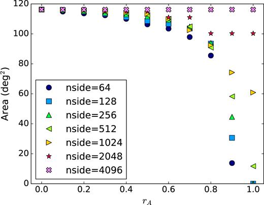
Area covered by different HEALpix pixellation resolutions as a function of the minimum fraction of pixel coverage of said resolution with respect to the Nside = 4096 footprint (larger pixels from lower Nside will be partially filled at times). This test is done using the MICE simulation considering the same footprint as the SV data set.
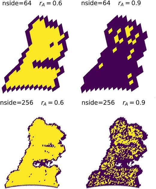
DES SV mask for different Nside (64, 256) and different area cuts rA = 0.6, 0.9. The pixels that we discard are blue and the ones that we keep are red. The bigger the pixel, the larger the amount of data we lose.
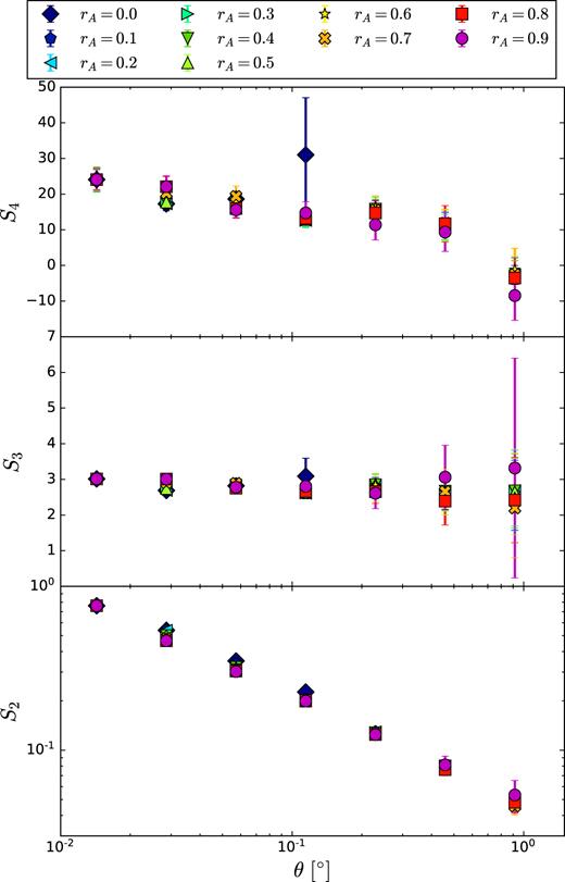
Moments of the density contrast distribution obtained from MICE (0.95 < |$z$| < 1.05) considering the same footprint as the SV data for different values of the fraction of the pixel inside the mask, rA. The results for a given scale θ have been separated in the figure for visualization purposes.
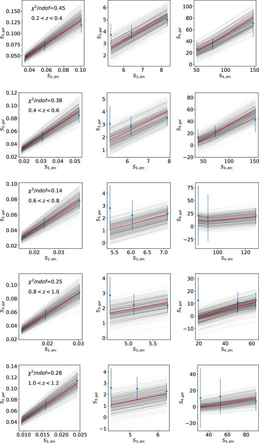
Fit results for the non-linear bias simultaneous fits method using MICE with Gaussian photo-z. The points are the measured moments and the error bars are calculated by adding in quadrature the uncertainties from the moments in the dark matter and the galaxies. The thick dark line is the best-fitting curve corresponding to the mean of the posterior distribution. The thin grey lines are the different models evaluated by the MCMC. The top row corresponds to the first redshift bin (0.2 < |$z$| < 0.4), the second row corresponds to the second redshift bin, and so on.
APPENDIX C: SIMULTANEOUS FITS RESULTS
In this section we show the fitting results for the simultaneous fits in MICE. In Figs C1 and C2, the red line corresponds to the mean value of the samples and the grey lines are the different models evaluated by the MCMC.
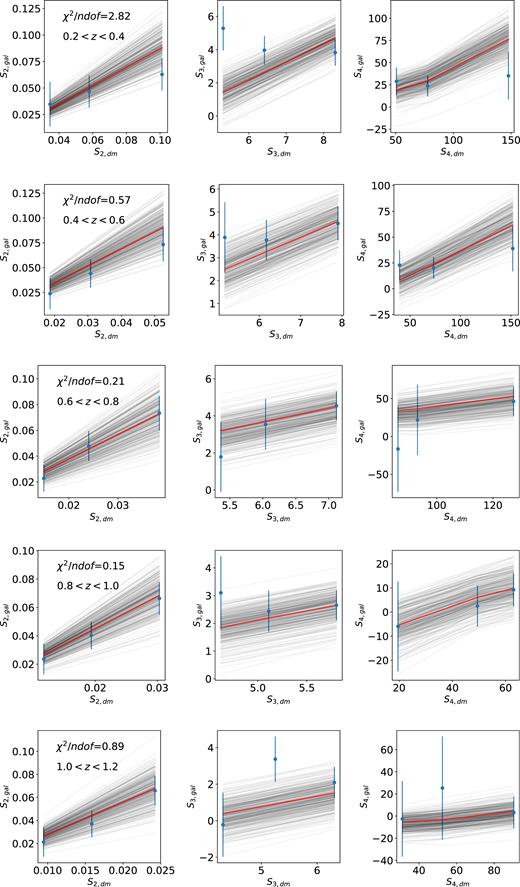
Non-linear bias fits for DES SV data. See caption in Fig. C1 for more details.
