


ABSTRACT
Ancient lunar appulse and occultation observations are analysed to derive new constraints on the difference between Terrestrial Time and Universal Time (ΔT). The new estimates are combined with literature values to produce an updated equation for calculating ΔT prior to the second century AD.
1 INTRODUCTION
Considerable progress has been made in recent decades concerning the quantitative analysis of ancient eclipse observations. In particular, solar eclipse observations have proven very useful for constraining ΔT (= TT−UT), the difference between Terrestrial Time and Universal Time (Stephenson, Morrison & Hohenkerk 2016). Despite this progress, the pace of discovery of ancient solar eclipse observations has slowed almost to a halt. Thus, any additional progress in this area is likely to come from observations other than solar eclipses.
Stephenson & Baylis (2012) noted that it is also possible to constrain ΔT from lunar occultation observations. The best sources of ancient astronomical observations are Babylonian, Chinese, Greek, and Roman. Stephenson & Baylis (2012) analysed ancient Chinese lunar occultation observations and concluded that their overall quality was not sufficient to constrain ΔT. However, Gonzalez (2017) analysed 15 ancient Babylonian lunar appulse and occultation observations, successfully obtaining several tight constraints on ΔT from them.
More recently, Morrison, Hohenkerk & Stephenson (2017) analysed seven Greek and Roman lunar occultation and appulse observations recorded by Ptolemy in the Almagest. Their purpose was to investigate the accuracy of the lunar tidal acceleration obtained by Fatheringham & Longbottom (1915) corrected for ‘the acceleration of the Sun’ and to constrain the acceleration of the Moon’s longitude. To accomplish this goal, they adopted the equation for ΔT published in Stephenson et al. (2016). Some lunar events have very weak dependence on ΔT, while others (e.g. those occurring during twilight and/or near the horizon) depend on both the lunar acceleration and ΔT. Their result is consistent with the currently accepted value of the acceleration of the Moon’s longitude.
We have two goals with this work. The first is to determine whether any of the ancient lunar occultations and appulses examined by Morrison et al. (2017) can also be used to constrain ΔT. A second goal is to derive an updated equation for ΔT from astronomical observations made prior to the second century. Currently, applications of the ΔT equation to periods prior to the eighth century BC require extrapolation. Thus, even small improvements to the ΔT equation will translate to substantially increased confidence of our calculations of the circumstances of ancient astronomical events. We describe the observations and our methods in Section 2. In Section 3 we discuss the derivation of a new equation for ΔT. In Section 4 we apply the new equation for ΔT to several historically important eclipses prior to the second century. We present our conclusions in Section 5.
2 DESCRIPTION OF OBSERVATIONS AND METHODS
Morrison et al. (2017) analysed seven lunar occultations and appulses occurring between the years −294 and +98. From the description of each event written in the Almagest, they were able to derive the observed ut and then compare it to the calculated ut. From these comparisons they calculated the average lunar acceleration value. In this work, we adopt the dates and observed ut values for the events listed in their table 1.
Our method of analysis closely follows that of Gonzalez (2017). We refer the reader to that work for the details of the computational methods employed therein. As the software we use implicitly incorporates the modern value of the lunar acceleration, it is not a parameter we adjust during the analysis. Instead, our analysis of each event begins with the observed ut value, date, and location given by Morrison et al. (2017). The circumstances of an event (altitude of the moon, altitude of the sun, visibility of the star) for a given ΔT are then calculated for the observed ut. Calculations are repeated for other values of ΔT to explore the sensitivity of the circumstances to ΔT.
Apart from ΔT, the only other unknown parameter affecting our calculations is the value of the visual extinction coefficient. Typical values range from 0.2 to 0.3 mag/airmass, but smaller and larger values are sometimes measured (Schaefer 1993). Below we explore visibilities over this range of extinction coefficient. Extinction affects the apparent brightness of a star, the amount of scattered moonlight, and night and twilight sky brightness. Still, the precise value of the visual extinction coefficient is secondary in importance compared to the reported ut. The results of our analysis of each event are presented below in chronological order. Translations from Morrison et al. (2017) are given for each event; the reader is referred to their paper for additional details of each event.
2.1 Individual events
−294 December 21 – Occultation of β Scorpii
At the beginning of the tenth hour, the Moon appeared to occult the northernmost of the stars in the forehead of Scorpius very precisely with its northern rim.
Timocharis reported observing the Moon occult β Scorpii with its northern limb. This would actually have been an appulse, rather than an occultation. The star would have been near the threshold of visibility in the vicinity of the Moon for typical visual extinction values. Morrison et al. (2017) concluded that Timocharis lost the star long before closest approach, based on the reported ut; our analysis confirms their conclusion. Given these uncertainties, no useful constraints on ΔT can be derived.
−293 March 9 – Occultation of Spica
At the beginning of the third hour, the Moon covered Spica with the middle of that edge of its disk which is towards the equinoctial rising point (i.e. the east), and that Spica, in passing through, cut off exactly the northern third of [the Moon?s] diameter.
Timocharis observed the nearly full Moon occult the bright star Spica from Alexandria. While the Moon did indeed occult Spica, it would not have been possible to see it (even with exceptionally low visual extinction). Spica was more than a magnitude fainter than the threshold visibility magnitude. Timocharis must have lost sight of it long before the Moon actually occulted it. No useful constraints on ΔT can be derived.
−282 January 29 – Occultation of Pleiades
Towards the end of the third hour (of night), the southern half of the Moon was seen to cover exactly either the rearmost third or (the rearmost) half of the Pleiades.
Timocharis observed the Moon occult several stars in the Pleaides, which Morrison et al. (2017) identify as η, 27, and 28 Tauri. Of these, only η Tauri could possibly have been visible near the Moon, but it would have been near the threshold of visibility. Given these uncertainties and the terseness of the report, no useful constraints on ΔT can be derived.
−294 December 21 – Occultation of β Scorpii
When as much as half an hour of the tenth hour had gone by and the Moon had risen above the horizon, Spica appeared exactly touching the northern point on [the Moon].
Timocharis observed an appulse between the Moon and Spica. Visibility calculations indicate that Spica should have been easily visible beside the waning crescent Moon’s northern horn. A hard upper limit of ΔT = 15 500 s is set by the visibility requirement at low altitude. The resulting ΔT from the observed ut is 11 750 ± 700 s.
+92 Novembe 29 – Occultation of Pleiades
At the beginning of the third hour of night, the Moon occulted the rearmost, southern part of the Pleiades with its southern horn.
Agrippa observed the occultation of the southern part of the Pleiades from Nicaea. Morrison et al. (2017) argue that the stars in this part of the Pleiades would not have been seen close to the Moon’s limb. Our visibility calculations confirm this; the stars are nearly 4 mag fainter than the visibility threshold. Thus, it was not possible for the observer to give an accurate time for the occultation. No constraints on ΔT can be derived.
+98 January 11 – Occultation of Spica
When the tenth hour [of night] was completed, Spica had been occulted by the Moon (for it could not be seen), but towards the end of the eleventh hour, it was seen in advance of the Moon?s centre, equidistant from the [two] horns by an amount less than the Moon?s diameter.
Menelaus observed from Rome the reappearance of Spica from behind the Moon. It should have been easily visible near the dark limb even for high values of visual extinction. A hard lower limit of 6400 s is imposed on ΔT from bright twilight. The resulting ΔT from the observed ut is 9450 ± 350 s.
+98 January 14 – Lunar alignment with Scorpius
Towards the end of the eleventh hour, the southern horn of the Moon appeared on a straight line with the middle and the southernmost of the stars in the forehead of Scorpius, and its centre was to the rear of that straight line and was the same distance from the middle star as the middle star was from the southernmost; it appeared to have occulted the northernmost of the stars in the forehead, since [this star] was nowhere to be seen.
Menelaus describes the alignment of the Moon with two stars in Scorpius (δ and π Scorpii) but notes that β Scorpii (a brighter star) was not visible. Morrison et al. (2017) speculate that the lack of the visibility of β Scorpii was due to the glare from the Moon, rather than from an occultation. Calculations for a low visual extinction coefficient of 0.2 mag/airmass put β Scorpii less than 0.3 mag from the threshold of visibility. Increasing it to 0.3 mag/airmass puts it right at the threshold. Thus, its lack of visibility is indeed very plausibly explained by the Moon’s glare. The most important constraint on ΔT is the alignment of the Moon with the two other stars in Scorpius at the reported ut. The resulting value of ΔT is 8500 ± 500 s.
In summary, we derived useful constraints on ΔT for three of the seven events reported by Morrison et al. (2017).
3 A REVISED EQUATION FOR ΔT
Stephenson et al. (2016) provide the most up-to-date calibrated equation for ΔT going back to ancient times. However, given the relatively small number of constraints on ΔT prior to the sixth century, the addition of just a few more tight constraints in this period can have significant impact. There are additional sources of constraints on ΔT not included by Stephenson et al. (2016).
Although we derived three new independent constraints on ΔT in this work, two of them are nearly simultaneous. Taking a weighted-average of the two events in the year +98 yields 9150 ± 300 s for ΔT. The value of ΔT assumed by Morrison et al. (2017) for this year is 9500 s. Our other new constraint on ΔT is 11, 750 ± 700 s for the year −282, for which Morrison et al. (2017) assumed 14 000 s. It is important to note that the constraints on ΔT derived in this work have statistical error bars associated with them, whereas ΔT constraints presented in Stephenson et al. (2016) and Gonzalez (2017) are upper and lower bounds.
Gonzalez (2017) derived constraints on ΔT from 15 Babylonian lunar appulse and occultation observations between the years −79 and −418. From these, we adopt a subset of 12 useful constraints in this work. 10 events have both upper and lower bounds on ΔT, one has an upper bound, and one a lower bound.
From Stephenson et al. (2016) we adopt two sets of ΔT constraints from their supplemental tables: (1) lower and/or upper bounds, (2) individual values with assigned weights of 10 or above. While Stephenson et al. (2016) present an extensive set of constraints on ΔT published prior to 2016, they didn’t include all of them. In particular, we can add to our present analysis the constraints from Tanikawa et al. (2010) and Sôma & Tanikawa (2016). The ΔT constraints collected together from these works are shown in Fig. 1 for the years spanning −800 to +600.
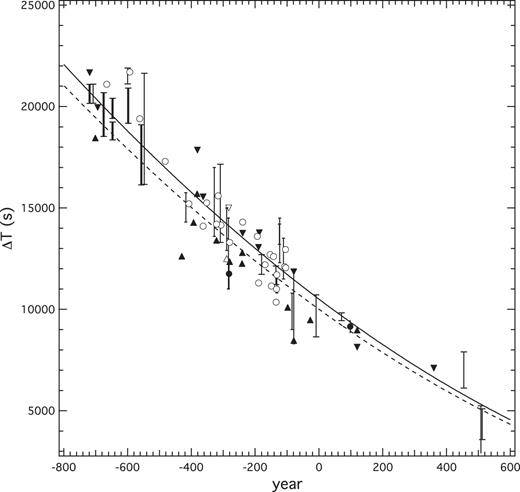
Constraints on ΔT from Stephenson et al. (2016) (bars with wide caps, open circles, solid triangles), Gonzalez (2017) (bars with narrow caps and open triangles), Tanikawa et al. (2010) (thick bars), Sôma & Tanikawa (2016) (two bars near year 500), and this work (dots with capless error bars). The downward pointing triangles are upper limits, and the upward pointing triangles are lower limits. In total there are 77 constraints. The solid curve is based on equation (1) with a value of 32.5 for the α parameter. The dashed curve is based on a value of 31.
Quadratic curves representing the high and low estimates of α are shown in Fig. 1. The difference between the two curves is not large, but potentially important for some applications. For the year zero equation 1 with α = 32.5 yields a ΔT value about 500 s larger compared to the value with α = 31. The difference grows to 1200 s for the year −1000 and to 2200 s for the year −2000. In the following a new fit using all constraints shown in Fig. 1 is derived.
Stephenson et al. (2016) defined a quantity they termed δ(ΔT), which is the differences between the individual ΔT values and equation (1). If the data were completely explained by the simple parabolic fit, then δ(ΔT) would be equal to zero. While systematic patterns in δ(ΔT) have been demonstrated for observations obtained since the 17th century, Stephenson & Morrison (1995) were the first to claim to have detected significant patterns also for the older data. Stephenson et al. (2016) found that it is necessary to add additional terms to the simple quadratic equation to account for the variations in ΔT going back to the earliest eclipse observations. They chose to fit δ(ΔT) with cubic splines, each applicable to a specific range of years. Their earliest polynomial fit ranges from the years −720 to +400. Their complete fit, ranging to the present, resembles a periodic function with a period near 1400 yr and an amplitude near 500 s.
A0 = = 500.0 s
T == 1400 yr
ϕ = = 5.9 radians
Thus, the only free parameter remaining is α. If the data were restricted to ordinary values with associated uncertainties, it would be straight-forward to determine the value of α with a non-linear least-squares analysis. However, there are three types of data we are using to constrain ΔT from the observations: upper or lower bound, upper and lower bounds, and standard deviation. We use the following approach to determine α. We perform non-linear least squares analysis on each of a large number of randomly drawn samples consistent with the various observed constraints on ΔT. For an event with both upper and lower bounds, a value is drawn at random with uniform probability between the bounds. An event with either an upper or a lower bound is treated in much the same way, except that ΔT is limited to values greater than 3000 and less than 25 000 s, respectively. An event with an associated uncertainty, instead of bounds, is sampled with a Normal distribution.
This approach generates data samples with obvious outliers. Therefore, we must employ a least-squares fitting method that is insensitive to outliers. To this end we use the pythonscipy robust non-linear regression package.2 The method is described in Triggs et al. (2002). We adopted the ‘soft_l1’ loss function. From a fit to 77 constraints, we determined that α = 32.7 ± 0.4 s cy-2. This is consistent with the value determined by Stephenson et al. (2016), but with a significant reduction in the uncertainty.
Fig. 2 is a plot of δ(ΔT) for α = 32.7. The figure should be compared to fig. 15 of Stephenson et al. (2016). From this, we see that the inclusion of δ(ΔT) in our solution is still justified. The fit to δ(ΔT) reaches a minimum near the year −300, and the bulk of the constraints tend to bias toward negative values in this time period. Particularly important are the tight constraints in the first century and near the year −130. Most other constraints display a scatter in δ(ΔT) that is larger than the amplitude in equation (2). However, taken together, the constraints limit the amplitude during this period to a value below 700 or 800 s.
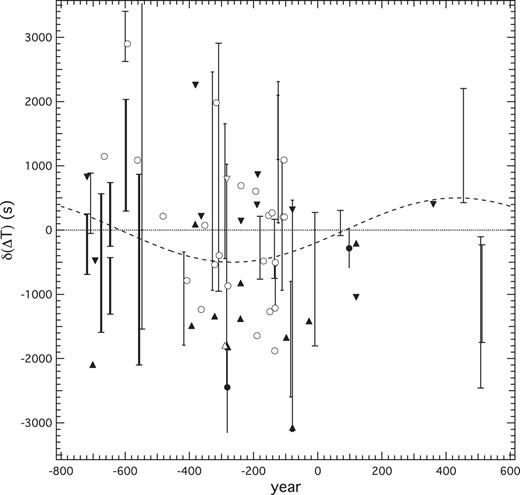
δ(ΔT) for the same data plotted in Fig. 1. The horizontal dotted line is the quadratic fit from equation (1) with α = 32.7. The dashed curve represents equation (2).
Leaving out equation (2) from the fit results in a slight reduction in the best-fitting value of α, to 32.4. This explains a portion of the difference between the values of α suggested by Gonzalez (2017) and Stephenson et al. (2016).
4 CONCLUSIONS
We have derived two new constraints on ΔT prior to the second century. From these, as well as 75 additional high quality constraints from the literature prior to the sixth century, we have calculated a new value for the coefficient, α, to the quadratic term of the equation for ΔT. We determine that α = 32.7 ± 0.4 s cy-2. This is consistent with the value determined by Stephenson et al. (2016) but with significantly reduced uncertainty.
Our new equation for ΔT can be used to determine the circumstances of historically important astronomical observations prior to the second century with greater confidence.
ACKNOWLEDGEMENTS
We thank the reviewer for helpful comments and suggestions.
Footnotes
Note, Gonzalez (2017) did not perform a formal analysis of the α parameter.
