


ABSTRACT
We present tables of velocity dispersions derived from CALIFA V1200 datacubes using Pipe3D. Four different dispersions are extracted from emission (ionized gas) or absorption (stellar) spectra, with two spatial apertures (5 and 30 arcsec). Stellar and ionized gas dispersions are not interchangeable and we determine their distinguishing features. We also compare these dispersions with literature values and construct sample scaling relations to further assess their applicability. We consider revised velocity-based scaling relations using the virial velocity parameter |$S_{K}^2 = K V_{\mathrm{ rot}}^2 + \sigma ^2$| constructed with each of our dispersions. Our search for the strongest linear correlation between SK and i-band absolute magnitudes favours the common K ∼ 0.5, though the range 0.3–0.8 is statistically acceptable. The reduction of scatter in our best stellar mass-virial velocity relations over that of a classic luminosity–velocity relation is minimal; this may however reflect the dominance of massive spirals in our sample.
1 INTRODUCTION
The burgeoning field of integral field spectroscopy (IFS) is enabling spatially resolved spectroscopy for unprecedentedly large collections of galaxies. The Calar Alto Legacy Integral Field spectroscopy Area (CALIFA) survey (Sánchez et al. 2012; Walcher et al. 2014; Sánchez et al. 2016c) is a forefront contributor to this movement, being the first completed IFS survey to target a diverse sample of galaxies in the local Universe and covering the entire Hubble sequence.
Pipe3D (Sánchez et al. 2016a,b) is a pipeline designed to model the stellar populations and ionized gas of a galaxy using optical integral field unit (IFU) observations. It can apply to spectral data from a wide range of IFS surveys, such as MaNGA (Bundy et al. 2015; Abolfathi et al. 2018; Sánchez et al. 2018), SAMI (Bryant et al. 2015), and other IFS data sets such as the one provided by MUSE (Sánchez-Menguiano et al. 2018) in addition to CALIFA (Cano-Díaz et al. 2016; Sánchez et al. 2016c; Bolatto et al. 2017). The goal of this study is to re-examine the stellar (absorption) velocity dispersions obtained in the preliminary extraction steps of Pipe3D, prior to fitting simple stellar population (SSP) templates for population studies, as well as the gaseous velocity dispersions measured during the modelling of emission lines.
Although Pipe3D was not specifically developed for kinematic studies, the absorption and emission velocity dispersions are a natural by-product of the modelling process. It is thus of interest to make use of these velocity dispersions to expand Pipe3D’s range of applications and assess the reliability of the extracted velocities.
SK is an alternate tracer of a galaxy’s potential that takes into account contributions from ordered rotation and random motions (Weiner et al. 2006; Kassin et al. 2007). Among others, it has been used to study the redshift evolution of scaling relations [particularly the velocity–luminosity or ‘Tully–Fisher’ relation of spiral galaxies (Tully & Fisher 1977)], since distant galaxies exhibit complex forms of rotational and pressure support (Cresci et al. 2009). However, it is unclear whether SK applies or provides any improvements over Vrot in this context (Miller et al. 2011). SK has also been used for the unification of local galaxies of diverse morphology into a common dynamical framework (Aquino et al., submitted; Zaritsky, Zabludoff & Gonzalez 2008; Cortese et al. 2014).
CALIFA and other IFS surveys afford the unique ability to assess the global rotation of a galaxy and the local velocity dispersion from the same spectral observations for a large sample of galaxies. The thorough testing of various forms of SK for local galaxies, in order to establish best practices for future work, is thus enabled here.
The organization of this paper is as follows. In Section 2, we introduce our sample and data, and compare our dispersions with one another. Those dispersion measurements are then contrasted with literature analogues in Section 3. Scaling relations of various forms are constructed in Section 4 to assess the utility and applicability of our dispersions as global kinematic tracers. We examine the virial kinematic tracer SK in Section 4.2 in the context of luminosity–velocity relations in order to determine an optimal value for K. We summarize our work in Section 5.
2 SAMPLE AND DATA
Our investigation of galaxy emission and absorption velocity dispersions takes advantage of the third CALIFA data release, employing a size-selected sample spanning a variety of environments in the local universe (out to |$z$| ∼ 0.03 for the main sample). Observations were carried out at the Calar Alto Observatory with the Potsdam Multi Aperture Spectrograph (PMAS) in the PPAK mode. The central hexagonal bundle contains 331 fibres, each 2.7 arcsec in diameter, with a total field of view of 74 × 64 arcsec. An additional 36 fibres in bundles of 6 cover the sky background. A three-pointing dithering pattern was used to cover the gaps between the fibres and increase the final resolution of the reduced datacubes to approximately 2.5 arcsec (1 kpc at the average redshift of CALIFA galaxies). The typical seeing was 1 arcsec FWHM. There are two low- and medium-spectral resolution observing modes for CALIFA: V500 and V1200 (for grisms with 500 lines mm−1 and 1200 lines mm−1, respectively). The low-resolution V500 observations span 3745–7300Å with R ∼ 850 at 5000Å. The medium-resolution V1200 observations span 3400–4750Å with R ∼ 1650 at 4500Å. A total of 667 galaxies were included in the third and final CALIFA data release (Sánchez et al. 2012, 2016c, 2017).
We have used Pipe3D (Sánchez et al. 2016a,b) to extract our measurements of stellar and gaseous dispersions for CALIFA galaxies, and now briefly describe the measurement procedure. The stellar velocity dispersion, σ*, is measured by fitting a small, representative set of stellar templates to the entire spectrum. The systemic velocity, Vsys, is first measured by adopting a fixed velocity dispersion for the convolution with the stellar templates. The instrumental width (∼72 km s−1) is also convolved with the stellar templates. The systemic velocity is then held fixed while the best velocity dispersion is obtained by minimizing the reduced χ2. A bounded exploration is used in both cases. For the systemic velocity, the redshift range of CALIFA is adopted. For the velocity dispersion, we explore a range between 1–500 km s−1. With the dispersion and systemic velocity in place, the dust attenuation, A|$v$|, can also be derived using a limited set of stellar templates. Finally, knowing Vsys, σ*, and A|$v$|, the stellar populations are then fitted using a Monte Carlo approach (see Sánchez et al. 2016b, for further details).
Emission lines are modelled with a Gaussian function and a polynomial background in the residual spectrum after subtracting the fitted stellar spectrum. Portions of the spectrum containing one or two emission lines are fitted individually rather than fitting the entire spectrum at once, to keep the form of the polynomial background simple. The systemic velocity and velocity dispersion of any lines fitted simultaneously are fixed as equal. Limits to the systemic velocity of the emission lines are based on the values derived for the stellar systemic velocity, exploring a range of ±300 km s−1 from that value. The allowed range of the velocity dispersion is the same as that in the stellar case. The instrumental width is subtracted in quadrature from the emission line velocity dispersion after fitting.
Pipe3D yields eight different velocity dispersion measurements. These can be derived from either V500 or V1200 observations, fitted either in absorption (tracing stars) or in emission (tracing ionized gas), and measured either within a 5 arcsec diameter aperture or a 30 arcsec diameter aperture. Due to the size-selected nature of the CALIFA sample, galaxies at higher redshift also tend to be physically larger. Therefore, the distance covered in these apertures is roughly constant with respect to the scale length of the galaxies. The 5 arcsec aperture covers approximately 0.2 Re, and the 30 arcsec aperture covers approximately 1.2 Re.
For the gaseous velocity dispersions, the V500 lines of choice are [OIII] and H α whereas the V1200 sampling favours Hδ. We focus on the V1200-based dispersion measurements, as the lower resolution V500-based dispersions are unreliable, especially at lower values as a result of the relatively significant instrumental dispersion of this observing mode. These dispersions were extracted by one of us (SFS) and are presented in Table 1. We exclude any dispersions where the uncertainty on the measurement exceeds the measurement itself from our following analyses. Our results change minimally if these high error entries are included.
Table of V1200 velocity dispersions produced using FIT3D. V500-derived H α fluxes are also tabulated for reference. The first 20 rows of the table are shown here. The full version of this table is available online as supplementary material, as well as at: https://www.physics.queensu.ca/Astro/people/Stephane_Courteau/gilhuly2017/index.html.
| Name | 5 arcsec σ* | 30 arcsec σ* | 5 arcsec σHδ | 30 arcsec σHδ | 5 arcsec H α flux | 30 arcsec H α flux |
|---|---|---|---|---|---|---|
| (km s−1) | (km s−1) | (km s−1) | (km s−1) | (CGS) | (CGS) | |
| 2MASXJ01331766|$+$|1319567 | 16.6 ± 11.7 | 24.6 ± 11.9 | 114.6 ± 8.4 | 84.3 ± 11.6 | 34.7 ± 4.5 | 456.9 ± 44.0 |
| ARP220 | 160.7 ± 64.9 | 231.7 ± 23.2 | 191.7 ± 18.5 | 47.6 ± 5.0 | 668.0 ± 51.2 | |
| CGCG163-062 | 12.9 ± 11.7 | 110.7 ± 11.3 | 106.6 ± 9.6 | 16.1 ± 3.1 | 280.1 ± 31.4 | |
| CGCG251-041 | 142.6 ± 44.9 | 108.1 ± 20.7 | 171.8 ± 16.0 | 144.2 ± 21.6 | 231.0 ± 14.3 | 773.6 ± 85.4 |
| CGCG263-044 | 124.0 ± 15.3 | 103.6 ± 12.2 | 193.0 ± 26.3 | 172.1 ± 19.6 | 51.3 ± 3.6 | 233.7 ± 26.1 |
| CGCG429-012 | 129.2 ± 14.3 | 124.7 ± 12.8 | 25.3 ± 9.6 | 203.2 ± 82.3 | ||
| CGCG536-030 | 55.6 ± 12.0 | 15.1 ± 12.0 | 12.7 ± 1.8 | 73.9 ± 5.5 | 59.8 ± 4.4 | 1122.2 ± 56.9 |
| ESO539-G014 | 77.3 ± 38.3 | |||||
| ESO540-G003 | 83.9 ± 12.3 | 110.2 ± 21.4 | 154.0 ± 15.7 | 24.4 ± 12.4 | 894.9 ± 137.9 | |
| IC0159 | 206.4 ± 188.0 | 122.9 ± 50.9 | 56.7 ± 3.9 | 112.6 ± 13.5 | 1196.5 ± 64.2 | 7087.2 ± 607.4 |
| IC0195 | 130.9 ± 12.4 | 96.0 ± 12.3 | 12.8 ± 8.4 | 82.8 ± 77.0 | ||
| IC0307 | 224.3 ± 88.0 | 165.8 ± 24.8 | 195.8 ± 26.7 | 257.2 ± 15.4 | 66.0 ± 8.6 | 501.9 ± 86.4 |
| IC0480 | 103.8 ± 51.6 | 98.4 ± 69.9 | 82.6 ± 10.8 | 130.6 ± 17.4 | 28.0 ± 2.4 | 589.4 ± 47.7 |
| IC0485 | 259.0 ± 44.2 | 163.9 ± 17.3 | 169.9 ± 18.1 | 249.9 ± 12.4 | 70.4 ± 6.5 | 407.8 ± 46.6 |
| IC0540 | 81.1 ± 15.4 | 69.3 ± 12.1 | 51.7 ± 3.7 | 111.3 ± 10.2 | 43.3 ± 2.9 | 228.8 ± 35.7 |
| IC0674 | 188.6 ± 22.1 | 179.0 ± 13.2 | 211.8 ± 14.7 | 227.5 ± 28.6 | 32.3 ± 4.1 | 335.9 ± 51.5 |
| IC0776 | 55.9 ± 12.9 | 8.7 ± 11.6 | 110.3 ± 11.2 | 114.4 ± 9.1 | 1861.8 ± 110.7 | |
| IC0944 | 195.8 ± 13.4 | 201.0 ± 21.7 | 198.3 ± 21.6 | 240.1 ± 28.8 | 16.6 ± 3.1 | 172.6 ± 35.6 |
| IC1078 | 66.6 ± 62.7 | 217.2 ± 24.5 | 277.8 ± 21.2 | 16.2 ± 5.2 | 447.3 ± 93.9 |
The above dispersions are measured by fitting the sum of all spectra within the aperture. This procedure enhances signal-to-noise ratio (S/N), especially for the V1200 gaseous dispersions. However, if there is significant rotation within the aperture, the component projected along the line of sight will be added in quadrature with the dispersion (and instrumental dispersion) to yield a composite line width. In order to test the extent to which the above dispersions are contaminated with rotation, we have also calculated the mean of individually fitted spaxel dispersions (‘spaxel-wise’) for the 30 arcsec aperture dispersions. We assume the 5 arcsec dispersions are minimally contaminated.
Close agreement between the spaxel-wise and standard measurements of the V1200 30 arcsec aperture stellar dispersions indicates minimal contamination from rotation. Thus, we continue to use the standard dispersion measurement in this case. The V1200 30 arcsec aperture gaseous dispersions could not be remeasured due to insufficient S/N in the Hδ line for individual spaxels.
2.1 Stars versus gas
We now characterize and contrast our gaseous and stellar dispersions measured with a common aperture. Emission and absorption velocity dispersions are measured from tracers with typically different dynamical histories. The gas which gives rise to emission spectra is normally confined to the mid-plane of a galaxy and is dominated by rotational motions (the latter may suffer from non-circular perturbations; see Spekkens & Sellwood 2007). Gas spectra may also be broadened by non-dynamical sources such as hot stars, winds, turbulence, active galactic nuclei, etc. Spatially resolved emission lines thus inform us about the rotational movement of its source (centroid of the spectral line) as well as the heating of its source (width of the line). The spatially integrated emission spectrum, or global line width, of a galaxy is thus the reflection of various rotational and broadening mechanisms.
Stars may deviate from their original birth paths due to random stellar perturbations over their lifetime and exhibit asymmetric drift as a result. The spatially resolved and integrated absorption spectra are also affected by rotational and broadening mechanisms, in a manner that differs from emission spectra. For instance, feedback mechanisms and winds have little effect on stellar motions.
Given different sensitivities of stars and gas to local gravitational and thermal effects, and especially as those evolve over time, emission and absorption velocity dispersions are expected to trace different systems and thus differ from one another. As we revisit below, the two types of measurements cannot be used interchangeably.
Fig. 1 compares the stellar and gaseous velocity dispersions, for the same aperture size, where both dispersions are available. The correlation between these dispersions is generally weak. We note a tendency for galaxies with high absolute measurement error on σ to fall further from the best-fitting line than those with low absolute measurement error. However, the observed scatter is greater than can be explained by measurement errors alone.
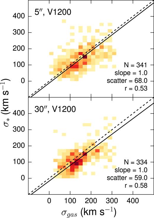
Comparison of Pipe3D V1200 gaseous and stellar velocity dispersions. The dashed line indicates a 1:1 relation while the solid line is the best linear fit to the data.
In order to examine the differences between these dispersions, we consider the galaxies with the best and worst match amongst stellar and gaseous measurements. This is done by plotting σgas − σ* against various ancillary data: apparent and absolute i-band magnitudes (Gilhuly & Courteau 2018), Hubble type (Walcher et al. 2014), star formation rate (Catalán-Torrecilla et al. 2015), mean stellar age at 1 Re, A, and mean stellar metallicity at 1 Re, Z (González Delgado et al. 2015). We do not find any trends in the residuals for σgas − σ* against all of the considered galaxy properties, suggesting a global lack of correlation between stellar and gaseous dispersions. The latter quantities must indeed be treated as distinct entities.
2.2 5 arcsec versus 30 arcsec aperture
Fig. 2 compares dispersion measurements for 5 and 30 arcsec apertures. Modulo a few outliers, the V1200 stellar dispersion shows very good agreement between our two aperture sizes for our stellar dispersions, with weaker agreement for the gaseous dispersions. We find a slight negative gradient in |$\sigma _{30\,{arcsec}}-\sigma _{5\,{arcsec}}$| for stellar dispersions towards higher age and metallicity in Fig. 3. Beyond A < 109 yr and Z < 1, the scatter in |$\sigma _{30\,{arcsec}}-\sigma _{5\,{arcsec}}$| for stellar dispersions appears to increase (signalling weaker correlation between the two dispersions). This suggests that the stellar dispersions are less reliable for galaxies with younger stars. The connection between stellar dispersions of differing apertures worsens significantly for Sc and later galaxies (though this may simply reflect the trends seen against age and metallicity).
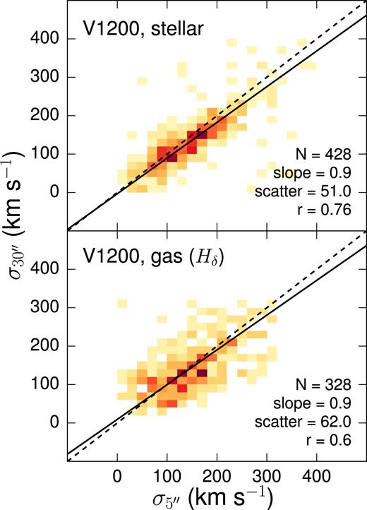
Comparison of Pipe3D V1200 velocity dispersions measured within 5 arcsec diameter and 30 arcsec diameter apertures. The dashed line indicates a 1:1 relation while the solid line is the best linear fit to the data.

While the overall scatter in |$\sigma _{30\,{arcsec}}-\sigma _{5\,{arcsec}}$| is greater for gaseous dispersions, we find no connections with other galaxy properties. This indicates less consistent variation in gaseous dynamics from central to the mid-outer regions of CALIFA galaxies compared to stellar dynamics.
We have demonstrated that the choice of stars versus gas and aperture size all impact the final measured dispersions, with the weakest agreement between stellar and gaseous dispersions. In general, these dispersions cannot be used interchangeably. A more detailed investigation is required to determine which dispersion measure is most reliable or most informative for a given scientific application, as we discuss in Section 3.
3 COMPARISON WITH EXISTING LINE WIDTHS
In order to validate our data and better understand their significance and applications, we now compare our dispersions with similar existing data products. First, we compare our gaseous dispersions with HI line widths from Springob et al. (2005), shown in Fig. 4. We use W50 from their catalogue, defined as the line width measured at 50 per cent of the peak flux. The peak flux and half-peak flux are measured separately for each half of the H i line profile, to better handle asymmetrical profiles. Dispersion, instrumental, and cosmological contributions to W50 have already been removed, leaving a (projected) measurement of the ordered rotation of a galaxy. We deproject and halve the corrected line widths to obtain an estimate of rotational velocity, V50.
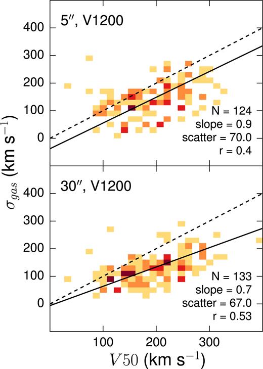
Comparison of Pipe3D gaseous velocity dispersions with H i rotation velocities derived by deprojecting and halving H i line widths from Springob et al. (2005). The dashed line indicates a 1:1 relation while the solid line is the best linear fit to the data.
We find a modest correlation between our dispersions (σ) and V50, as shown in Figs 4 and 5. The dispersions are expectedly smaller than V50, by ∼50 − 100 km s−1. Since the V50 estimates are measured at radii that are larger than the dispersion apertures, the interpretation of this correlation and whether it suffers any contamination from rotation is challenging. Besides the fact that rotational motions dominate over dispersion in disc galaxies, the lower values of σ relative to V50 may also be due to the smaller apertures over which dispersions are measured. At the very least, the linear correspondence between σ and V50 indicates that both are good tracers of the gravitational potential in these galaxies. The somewhat stronger correlation of V50 with σ* (relative to σgas) may reflect the weaker S/N of the Hδ lines compared to the stellar absorption lines in the V1200 datacubes.
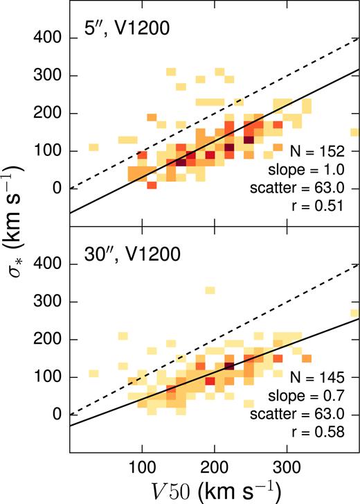
Comparison of Pipe3D stellar velocity dispersions with HI rotation velocities derived by deprojecting and halving H i line widths from Springob et al. (2005). The dashed line indicates a 1:1 relation while the solid line is the best linear fit to the data.
Fig. 6 compares our V1200 dispersions with the (stellar) dispersion maps of Falcón-Barroso et al. (2017) based on CALIFA V1200 datacubes. We derive approximate aperture dispersions from the maps by taking the average dispersion of all cells with centres within 2.5 arcsec or 15 arcsec of the centre of the galaxy. The averages are taken from Voronoi bins and are therefore flux weighted. Strong agreement is found with our V1200 5 arcsec stellar dispersions, with a reasonable match for our 30 arcsec stellar dispersions. Our approach to extracting an aperture dispersion and the necessarily larger size of the Voronoi bins relative to our apertures at greater separation from the galaxy centre may explain the somewhat poorer correlation between our 30 arcsec stellar dispersions relative to the 5 arcsec stellar dispersions. Establishing this favourable comparison reflects the quality of our dispersions. While a direct correspondence between stellar and gaseous dispersions (Section 2.1) is not expected, especially if radiative effects are strong, a reasonable correlation between our gaseous dispersions and the stellar dispersions of Falcón-Barroso et al. (2017) is still found, particularly for the smaller 5 arcsec aperture.
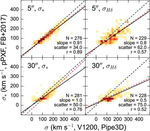
Comparison of Pipe3D velocity dispersions with the average velocity dispersion within comparable apertures from the maps generated by pPXF (Falcón-Barroso et al. 2017). The dashed line indicates a 1:1 relation while the solid line is the best linear fit to the all of the data. Due to the imposed minimum of 40 km s−1 in the pPXF maps, we also perform a secondary fit only on galaxies where both Pipe3D and pPXF measure σ > σinst (∼72 km s−1). This fit is shown in dashed red, and its best-fitting parameters are displayed in each panel. We note that the secondary fit is only significantly different from the first fit in the lower right panel, for the comparison with our 30 arcsec aperture stellar dispersions.
4 SCALING RELATIONS
We pursue our validation and comparison of our velocity dispersions by examining a selection of dynamical scaling relations. The tight correlation of independent galaxy properties with our velocity dispersions may further enhance our understanding of the physical processes governing galaxy formation and evolution. We make use of the extensive CALIFA photometry catalogue of Gilhuly & Courteau (2018) for total i-band magnitudes, effective surface brightnesses and radii, colours, stellar masses, and colours in order to construct various scaling relations and to verify for completeness.
4.1 Fundamental Plane
We consider the Fundamental Plane (FP), the characteristic dynamical scaling relation of early-type galaxies (Djorgovski & Davis 1987; Dressler et al. 1987; Cappellari et al. 2013; D’Onofrio et al. 2017). We adhere to the completeness limits of CALIFA (−19 > Mr > −23.1, see Walcher et al. 2014), and retain only elliptical and lenticular galaxies in the FP sample. Fig. 7 shows that the two FPs constructed using each of our stellar velocity dispersions successfully produce thin planes.
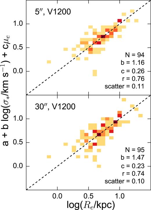
The CALIFA Fundamental Plane, viewed edge-on, generated using Pipe3D V1200 stellar velocity dispersions. Re and μe are sourced from the Gilhuly & Courteau (2018) CALIFA photometry catalogue. The dashed line corresponds to the fitted edge-on plane.
The slope parameters for the FPs are broadly consistent with the literature. For instance, b is typically measured as 1.06–1.55 (Djorgovski & Davis 1987; Dressler et al. 1987; Bernardi et al. 2003; La Barbera et al. 2008; Cappellari et al. 2013; Ouellette et al. 2017), encompassing our values of 1.16 and 1.47. b is typically found to decrease with larger apertures (Ouellette et al. 2017); however, our V1200 30 arcsec aperture FP b is closest to literature FPs constructed using the central velocity dispersion σ0 (Bernardi et al. 2003) while our V1200 5 arcsec aperture FP b is similar to FPs constructed with σ measured within Re (Cappellari et al. 2013; Ouellette et al. 2017). Considering the conversion from magnitudes to log Ie, typical values of c are 0.30–0.36. Our values of 0.23 and 0.27 may lie outside this range due to bandpass differences or the properties of our ETG sample (especially the number of galaxies and the mass range investigated). Overall, this agreement is encouraging given the small sample size.
4.2 SK and the Tully–Fisher relation
Unlike ETGs, LTGs are rotation dominated and their respective dynamical scaling relations take advantage of circular velocities. Therefore, the ranking and exploitation of these dispersions becomes more complicated for LTGs. We now turn to the Tully–Fisher relation which connects the circular rotation velocity Vrot and luminosity or stellar mass of disc galaxies (TFR: Tully & Fisher 1977; McGaugh et al. 2000; Courteau et al. 2007).
The potential of a dynamical system can be inferred by considering all stellar and gas motions. SK (equation 1) could be used as a complement to pure circular velocity (typically for the gas) to account for random (stellar) motions and potentially yield a tighter scaling relation with M* than the classic stellar mass TFR. While the most commonly used value for K is 0.5 (Weiner et al. 2006; Kassin et al. 2007; Cortese et al. 2014), we test 0.2 ≤ K ≤ 1.5 in increments of 0.1. The motivation for K = 0.5 comes from the expected relation between velocity dispersion and rotation velocity for a population of tracers that have a spherically symmetric distribution and isotropic velocity dispersion. If these conditions are met and ρ ∝ r−2, |$K = \frac{1}{2}$|. One might also argue for K = 0.33 from a consideration of kinetic energy. A rotating disc has |$E_K = \frac{1}{2} M v_{\mathrm{ rot}}^2$| while a pressure-supported spherical galaxy has |$E_K = \frac{3}{2} M \sigma _{v}^2$|. If support from both rotation and pressure are considered, the relative weighting would therefore be 3 to 1, yielding |$K=\frac{1}{3}$|.
In order to apply (equation 1), we use Vmax from the gas (H α) rotation curve analysis of Holmes et al. (2015) for galaxies within the completeness limits of the CALIFA Data Release 1. Although Holmes et al. focused on mid-inclination galaxies, we apply our own inclination cut of 40° < i < 80° to ensure that only the most reliable rotation curves are retained. As these rotation curves trace the gas emission, the sample is dominated by gas-rich spiral galaxies and early-type galaxies are poorly represented.
Examination of the reduced χ2 of our various M* − SK relations in Fig. 8 reveals that our V1200 gaseous dispersions combined with a gaseous Vmax fail to produce tighter linear correlations than the classic TFR; in fact they degrade the TFR, such that the ideal value of K is as large as possible to minimize the contribution of σ. This is at least partially attributed to the morphologically tight, spiral-dominated sample for which H α rotation curves were available.
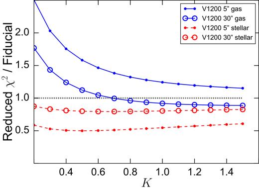
Change in the reduced χ2 of the M* − SK relation with increasing K for each dispersion, normalized against the reduced χ2 of the stellar mass TFR (i in dotted black). Only the V1200 stellar dispersions (dashed red) provide significant improvement over the stellar mass TFR. In this work, SK is always constructed with Vmax measured from H α rotation curves.
Of the 5 and 30 arcsec aperture V1200 stellar dispersions, the smaller aperture yields the greatest improvement in correlation strength relative to the TFR when combined with a gaseous Vmax to form SK. The reduced χ2 of the fitted M* − SK for both apertures reaches its minimum for K = 0.5, though there is very little variation over the interval 0.3 ≤ K ≤ 0.8. A comparison of the stellar mass TFR and our tightest M* − SK relation is shown in Fig. 9. The measured orthogonal scatter from the best-fitting M* − SK linear relation is reduced by 0.02 dex relative to that of the stellar mass TFR. It must be noted that the scatter of the stellar mass TFR was already quite low due to the spiral-dominated nature of this sample. A diverse sample, inclusive of ETGs and spanning a wider range of masses, could yield a relatively tighter M* − SK relation (Aquino et al., submitted).
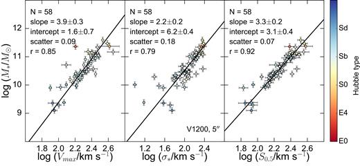
A revised TFR using SK as the kinematic tracer (shown in the right-hand panel). In the left-hand panel, we show our stellar mass TFR constructed using Vmax (Holmes et al. 2015). The centre panel shows the M* − σ relation using the V1200 5 arcsec stellar velocity dispersion. The final panel depicts the M* − SK relation, taking K = 0.8 (the value that results in the lowest reduced χ2). The solid lines show the best linear fits to the data. All points are colour-coded by Hubble type (Walcher et al. 2014).
Cortese et al. (2014) find that the M* − S0.5 relation constructed with stellar or gaseous kinematics results in a scaling relation that is tighter than the baryonic TFR or the Faber–Jackson relation for 235 SAMI galaxies of mixed morphology. They state that the scatter does not change for 0.3 < K < 1. Our results also corroborate that a wide range of K values yield similarly tight M* − SK relations. Our measured slope (3.3 ± 0.2) and that of Cortese et al. (3.0 ± 0.1) are consistent within error.
The galaxies studied by Cortese et al. have lower stellar masses and velocities than ours; this difference is significant since the relative contribution of ordered and dispersive stellar motions changes for less massive galaxies. The differences between CALIFA and SAMI observations (spectral resolution and coverage; spaxel size; radial coverage) and the techniques for measuring a rotation velocity may also contribute to our different results. For instance, we combine gas rotation velocities with stellar velocity dispersions while Cortese et al. do not. Furthermore, our gaseous and stellar velocity dispersions clearly differ; for Cortese et al., S0.5,gas and S0.5, * are a close match (see their Fig. 3c). Similarly, we do not consider any stellar rotation velocity for the construction of SK, which penalizes our analysis against early-type galaxies.
Our tests have exploited the CALIFA library for well-behaved low redshift galaxies, and adopting SK instead of Vrot is likely less impactful than for high redshift and/or less massive galaxies. Furthermore, we are limited in our ability to test SK for the unification of early- and late-type galaxies by the small number of ETGs with significant ordered rotation traced in H α emission (Holmes et al. 2015). A larger sample with Vrot measured for the stellar component in addition to H α may be needed to complete this study of SK.
5 SUMMARY
A table of dispersions measured in emission and absorption, tracing ionized gas and stars respectively, has been presented for CALIFA galaxies. The data can be retrieved at this website: https://www.physics.queensu.ca/Astro/people/Stephane_Courteau/gilhuly2017/index.html.
Four different types of measurements are available, either from stellar absorption or gaseous emission and using either 5 or 30 arcsec apertures. We note that every type of measurement may not be available for each galaxy.
We have attempted to better contrast the distinguishing features of these dispersion measurements. Dispersions measured in emission or absorption trace different emitters and thus different dynamics. Galaxies with younger stellar populations (roughly Z < 1 and A < 109 yr) may suffer from poorly constrained stellar dispersions and require special attention. The Fundamental Planes constructed with our V1200 stellar dispersions agree well with the ensemble of related studies in the literature, and no strong preference for the 5 or 30 arcsec aperture is found for this purpose. We have also considered a modified TFR where Vrot is replaced by the virial estimator SK for each of our dispersions and for 0.2 ≤ K ≤ 1.5. Our measured dispersions do not result in a greatly tighter M* − SK relation than the classic TFR, but this may be related to the limited nature of our spiral-dominated sample, with its small mass range and lack of a stellar rotation velocity to compliment the H α rotation curves of Holmes et al. (2015). The SK produced with 5 arcsec V1200 stellar velocity dispersions result in an M* − SK relation with the most improved goodness of fit over the classic TFR (Fig. 9). Using these dispersions, we find that 0.3 ≤ K ≤ 0.8 produce the tightest relations. The improvement in scatter would be better probed with a wider mass range and better representation of gas-poor systems.
SUPPORTING INFORMATION
CALIFA_V1200_dispersions.csv
Please note: Oxford University Press is not responsible for the content or functionality of any supporting materials supplied by the authors. Any queries (other than missing material) should be directed to the corresponding author for the article.
ACKNOWLEDGEMENTS
We thank L. Holmes for providing us with machine-readable files containing the rotation curves presented in Holmes et al. (2015). CG and SC acknowledge support from the Natural Science and Engineering Research Council (NSERC) of Canada through a PGS D scholarship and a Research Discovery Grant, respectively. SFS thanks the Consejo Nacional de Ciencia y Tecnología (CONACyT) program CB-285080 and DGAPA-UNAM IA101217 grant for their support to this project.
