


Abstract
Galaxy mergers are believed to trigger strong starbursts. This is well assessed by observations in the local Universe. However, the efficiency of this mechanism has poorly been tested so far for high-redshift, actively star-forming, galaxies. We present a suite of pc-resolution hydrodynamical numerical simulations to compare the star formation process along a merging sequence of high- and low-redshift galaxies, by varying the gas mass fraction between the two models. We show that, for the same orbit, high-redshift gas-rich mergers are less efficient than low-redshift ones at producing starbursts; the star formation rate excess induced by the merger and its duration are both around 10 times lower than in the low gas fraction case. The mechanisms that account for the star formation triggering at low redshift – the increased compressive turbulence, gas fragmentation, and central gas inflows – are only mildly, if not at all, enhanced for high gas fraction galaxy encounters. Furthermore, we show that the strong stellar feedback from the initially high star formation rate in high-redshift galaxies does not prevent an increase of the star formation during the merger. Our results are consistent with the observed increase of the number of major mergers with increasing redshift being faster than the respective increase in the number of starburst galaxies.
1 INTRODUCTION
Observations of star-forming galaxies show that they follow a tight correlation between their stellar mass (M⋆) and their star formation rate (SFR). This relation defines a main sequence (MS) that is observed over a wide redshift range (z = 4–0; Elbaz et al. 2007; Noeske et al. 2007; Peng et al. 2010; Rodighiero et al. 2011; Schreiber et al. 2015).
Outlier galaxies, which display higher specific star formation rate (sSFR) than members of the MS, correspond to the starbursting galaxies. Detailed observations of these galaxies in the local Universe show that, above a certain luminosity threshold (LIR > 1012 L⊙, which defines the ultraluminous infrared galaxies; see e.g. Houck et al. 1985), all galaxies are undergoing a major merger event (Armus, Heckman & Miley 1987; Sanders & Mirabel 1996; Ellison et al. 2013). It should also be noted that if all local starburst galaxies are undergoing an interaction it is not reciprocal, as all observed major mergers do not show a massive enhancement of star formation (at low redshift, see Bergvall, Laurikainen & Aalto 2003; at high redshift, see Jogee et al. 2009). This might however be due to a short extent of the starburst phase relative to the interaction time-scale.
Observations of star-forming galaxies have shown that the number of star-forming galaxies in the starbursting regime above the MS remains fairly constant (between 2 and 4 per cent) in the redshift range z = 4–0, with no or only weak variation with redshift; about twice at most between z = 0 and 2 (Rodighiero et al. 2011; Schreiber et al. 2015). Given that the major merger rate is thought to be an increasing function of redshift (Le Fèvre et al. 2000; Kampczyk et al. 2007; Kartaltepe et al. 2007; Lotz et al. 2011, and references therein), this implies that the efficiency of major mergers in triggering starbursts must decrease with increasing redshift. This hypothesis is backed by observations showing that major mergers are inefficient at driving star formation at z ≃ 2 (Kaviraj et al. 2013; Lofthouse et al. 2016) and calls for a detailed study of physical processes at play in galaxy major mergers, and their dependence on redshift.
Observations of local advanced mergers show that most of the star formation is concentrated in the inner regions (Sanders & Mirabel 1996; Duc, Mirabel & Maza 1997). These nuclear starbursts are explained by gravitational torques induced by the close interaction between the galaxies (Barnes & Hernquist 1991). However, gravitationally driven gas inflows alone cannot explain observations of an extended, off-nuclear increase of interaction-induced star formation (Barnes 2004; Chien & Barnes 2010; Smith et al. 2014). One of the most striking cases is the well-studied Antennae system, which is observed during the second pericentre passage (Renaud et al. 2008) and where the majority of star formation happens in dense clumps outside of the nuclei and in the overlap region (see e.g. Whitmore & Schweizer 1995). Atomic and molecular gas observations (such as Elmegreen et al. 2016a, for the NGC 2207–IC 2163 interacting pair) show that their star-forming regions have very dense molecular phases, which hints for strong gas compression.
Massive high-redshift (z > 2) galaxy discs are characterized by a high gas fraction: fgas ≃ 50 per cent at z = 2 to be compared with fgas ≃ 10 per cent at z = 0 (Daddi et al. 2010; Tacconi et al. 2010). This higher gas fraction makes the disc more prone to gravitational instabilities; the velocity dispersion is higher (σ ≃ 40 km s−1 at z = 2; Förster Schreiber et al. 2009; Price et al. 2016; Stott et al. 2016, to be compared with σ ≃ 10 km s−1 at z = 0) and the violent disc instability (VDI) induces strong nuclear inflows (Bournaud et al. 2012) and the formation of giant star-forming clumps of 107–109 M⊙(Elmegreen et al. 2007; Genzel et al. 2008; Elmegreen 2009; Magnelli et al. 2012; Guo et al. 2015; Zanella et al. 2015). At this redshift, it is hard to study the evolution of the galaxy morphology during encounters (see e.g. Cibinel et al. 2015), and especially the efficiency of gas fragmentation and nuclear inflows which trigger the starburst at low redshift.
Numerical simulations are particularly well suited to capture the complex and rapidly evolving dynamics of mergers. It has been shown that the spatial resolution plays an important role in the study of extended star formation (Di Matteo et al. 2008; Teyssier, Chapon & Bournaud 2010; Bournaud et al. 2011); one should be able to resolve the local Jeans length with several resolution elements to be able to capture the off-nuclei gas condensations that might also form stars. Merger simulations with resolution of a few 10 pc to pc-scale (Teyssier et al. 2010; Powell et al. 2013; Renaud et al. 2014, R14 in the following) yield an extended star formation, which is explained by an increase in the cold gas turbulence, and especially of its compressive mode, driven by interaction-induced fully compressive tides (Renaud et al. 2008, 2009). This process adds to the torque-driven gas inflows towards the nuclei in the enhancement of the SFR. Fragmentation of the gas is relatively more important than nuclear inflows at the first pericentre passages, when the impact parameter and the relative velocity are large, resulting in weak and short-lived gravitational torques.
Previous simulations of galaxy major mergers with a high gas fraction hint for a weak enhancement of star formation, in both burst amplitude and duration (see e.g. Bournaud et al. 2011; Hopkins et al. 2013; Scudder et al. 2015), or even not at all (Perret et al. 2014). However, they did not compare their sample to low gas fraction major mergers or investigate the physical cause of this mild burst.
In this paper, we present a comparison between low- and high-redshift major mergers using hydrodynamical simulations. We present two sets of simulations: one with a high gas fraction and one with a low gas fraction. We study the evolution of the properties of their star formation activity during the interactions. Section 2 presents the numerical simulation parameters. Section 3 describes the resulting evolution of the star formation activity during the interactions, and compares the high and low gas fraction cases. The analysis of the physical processes having a role in the star formation is presented in Section 4. Discussion and conclusions are drawn in Sections 5 and 6.
2 SIMULATIONS
2.1 Numerical technique
We perform the simulations using the adaptive mesh refinement (AMR) code ramses (Teyssier 2002). The overall method is analogous of that in Renaud, Bournaud & Duc (2015).
The coarsest grid is composed of 643 cells in a cubic box of 200 kpc, and we allow up to 10 further levels of refinement. This results in a maximum spatial resolution of 6 pc. A resolution study to discuss this choice is presented in Appendix A. Star and dark matter (DM) particles are also implemented in the initial conditions (see Section 2.2). We call the former old stars, to differentiate them from the new stars, that are formed during the simulation. A grid cell is refined if when there are more than 40 initial condition particles, or if the baryonic mass, including gas, old and new stars, exceeds 8 × 10⁵ M⊙. Furthermore, we ensure that the Jeans length is always resolved by at least four cells, by introducing a numerical pressure through a temperature floor set by a polytrope equation of state at high density (T∝ρ2), which is called Jeans polytrope thereafter, which prevents numerical fragmentation (Truelove et al. 1997). Such a polytrope was also added in numerous previous numerical simulations (Dubois & Teyssier 2008; Renaud et al. 2013; Bournaud et al. 2014; Kraljic et al. 2014; Perret et al. 2014).
The thermodynamical model, including heating and atomic cooling at solar metallicity,1 is the same as described in Renaud et al. (2015).
If the gas reaches a certain density threshold, ρ0, and if its temperature is no more than 2 × 10⁴ K above the Jeans polytrope temperature at the corresponding density, it is converted into stellar particles following a Schmidt law, |$\dot{\rho }_{\star } = \epsilon (\rho _{\mathrm{gas}} / t_{\mathrm{ff}})$| (Schmidt 1959; Kennicutt 1998), with ε the efficiency per free fall time set to 1 per cent, and |$t_{\mathrm{ff}} = \sqrt{3\pi / (32G\rho )}$| the free-fall time. The density thresholds (ρ0 = 30 cm−3 and ρ0 = 1e5 cm−3 for low and high gas fraction cases) are chosen to correspond to the isolated discs being on the disc sequence of the Schmidt–Kennicutt diagram (Daddi et al. 2010; Genzel et al. 2010), that is an SFR of ≃ 1M⊙ yr−1 (resp. ≃60M⊙ yr−1) in the low gas fraction case (resp. high gas fraction case) for each galaxy before the interaction. The difference in the normalization of ρ0 originates from the different gas mean density between the two cases.2
Because of the spatial resolution and the computational cost it would imply, we do not resolve individual star formation. We chose a high enough sampling mass for the new stars, i.e. higher than 1000 M⊙, so that we do not need to resolve the initial mass function.
In these simulations, we model three types of stellar feedback.
Photoionization from H ii regions (as in Renaud et al. 2013): UV photons from the OB-type stars ionize the surrounding gas. To model this process, we evaluate the radius of the Strömgren (1939) sphere around the newly formed stellar particle and heat up the gas to |$T_{\mathrm{ H\,\small {II}}} = 2 \times 10^{4}$| K.
Radiation pressure (as in Renaud et al. 2013): inside each H ii region, the scattering of photons on the gas acts as a radiative pressure. To model this process, we inject a radial velocity kick for each cell inside the Stromgren sphere.
Type-II supernova (SN) thermal blasts (as in Dubois & Teyssier 2008; Teyssier et al. 2013): stars more massive than 4 M⊙ eventually explode as Type II SNe (Povich 2012). We assume that 20 per cent of the initial mass of our stellar particle is in massive stars, and will be released 10 Myr after the formation of the stellar particle. On top of the mass-loss, we inject thermally a certain amount of energy in the cell: ESN = 1051 erg/10 M⊙.
This implementation of stellar feedback is therefore physically motivated, although subgrid. It has been used in numerical simulations of high gas fraction disc galaxies similar to ours, and was shown to have realistic effects on the galaxies, such as producing large-scale outflows with a mass-loading factor close to unity (Roos et al. 2015, and see section 3.3 and fig. 5 in Bournaud 2016), which is consistent with observations (see e.g. Newman et al. 2012).
2.2 Modelling low- and high-redshift galactic discs
We run a suite of massive galaxy merger simulations for gas-rich (fgas = 60 per cent) and gas-poor discs (fgas = 10 per cent). These gas fractions are typical of z = 2 and 0 disc galaxies. We chose to modify solely the gas fraction in order to isolate the effect of this parameter, and neglect the other differences between the low- and high-redshift, such as galaxy size, mass, and interaction parameters. These parameters are discussed in Section 5.2.3. Furthermore, it must be noted that we do not change the stellar mass of the bulge, so that the velocity profile and the galactic shear stay the same, and so that the low and high gas fraction orbits are as similar as possible.
The DM halo for each galaxy is composed of 2.62 × 10⁵ M⊙ particles, following a Burkert (1995) profile. An old stellar component is added, made of 9 × 10⁴ M⊙ particles modelling a stellar disc and a stellar bulge. The characteristics of the galaxies are summed up in Table 1. The DM, old stars, and the stellar particles formed during the simulation are evolved through a particle-mesh solver, with a gravitational softening of 50 pc for the DM and old stars and at the resolution of the local resolution for the new stars.
Characteristics of the galaxies used in the simulations.
| Galaxy | Low gas fraction | High gas fraction |
|---|---|---|
| Total baryonic mass (×109 M⊙) | 57.2 | |
| Gas disc (exponential profile) | ||
| Mass (×109 M⊙) | 5.0 | 34.3 |
| Characteristic radius (kpc) | 8.0 | |
| Truncation radius (kpc) | 14.0 | |
| Characteristic height (kpc) | 0.3 | |
| Truncation height (kpc) | 0.8 | |
| Stellar disc (exponential profile) | ||
| Number of particles | 500 000 | 173 900 |
| Mass (×109 M⊙) | 45.0 | 15.7 |
| Characteristic radius (kpc) | 5.0 | |
| Truncation radius (kpc) | 12.0 | |
| Characteristic height (kpc) | 0.34 | |
| Truncation height (kpc) | 1.02 | |
| Bulge (Hernquist profile) | ||
| Number of particles | 80 000 | |
| Mass (×109 M⊙ ) | 7.2 | |
| Characteristic radius (kpc) | 1.3 | |
| Truncation radius (kpc) | 3.0 | |
| DM halo (Burkert profile) | ||
| Number of particles | 500 000 | |
| Mass (×109 M⊙ ) | 131.0 | |
| Characteristic radius (kpc) | 25.0 | |
| Truncation radius (kpc) | 45.0 | |
2.3 Characteristics of the orbits
Our simulation sample comprises three orbits. Their parameters are summarized in Tables 2 and 3. The full simulation suite is summarized in Table 4. Low and high gas fraction mergers are run on the same reference orbit #1 for comparison. This orbit is close to that of the Antennae system, which was shown by R14 to be favourable to a strong starburst for low gas fraction discs. Orbits #2 and #3 have lower orbital energy, obtained by reducing the impact parameter and relative velocity by 15 and 30 per cent. This ensures that the results do not depend on an unforeseen particularity of the orbit. The initial orbital conditions are summarized in Table 2.
Initial conditions of the orbits.
| Galaxy 1 | Galaxy 2 | |
|---|---|---|
| Orbit #1 | ||
| Centre (kpc) | (10.55, −30.34, 46.68) | (−15.01, 30.44, −46.34) |
| Velocity (km s−1 ) | (−26.95, 23.23, −71.76) | (26.02, −23.28, 71.35) |
| Orbit #2 | ||
| Centre (kpc) | (8.64, −25.78, 39.71) | (−13.10, 25.89, −39.36) |
| Velocity (km s−1 ) | (−22.98, 19.74, −61.03) | (22.05, −19.80, 60.61) |
| Orbit #3 | ||
| Centre (kpc) | (6.21, −20.01, 30.87) | (−10.67, 20.11, −30.52) |
| Velocity (km s−1 ) | (−17.94, 15.32, −47.43) | (17.01, −15.37, 47.02) |
Orientations of the spin axis.
| Spin | Galaxy 1 | Galaxy 2 |
|---|---|---|
| dd | (−0.67, −0.71, 0.20) | (0.65, 0.65, −0.40) |
| rr | (0.67, 0.71, −0.20) | (−0.65, −0.65, 0.40) |
| Spin1 | (−0.67, 0.71, −0.20) | (−0.65, 0.65, 0.40) |
| Spin2 | (0.67, −0.71, 0.20) | (−0.65, −0.65, 0.40) |
| Spin3 | (0.67, 0.71, 0.20) | ( 0.65, −0.65, 0.40) |
| Spin4 | (−0.67, 0.71, −0.20) | (−0.65, −0.65, −0.40) |
Summary of the simulations. The prefix ‘gp’ stands for gas-poor. dd and rr stand for direct–direct and retrograde–retrograde, and are followed by the number of the corresponding orbit.
| Name | Orbit | Spins | Gas fraction | Maximum resolution (pc) |
|---|---|---|---|---|
| Iso | – | – | 60% | 6 |
| gp-iso | – | – | 10% | 6 |
| dd1 | 1 | dd | 60% | 6 |
| rr1 | 1 | rr | 60% | 6 |
| gp-dd1 | 1 | dd | 10% | 6 |
| gp-rr1 | 1 | rr | 10% | 6 |
| dd2 | 2 | dd | 60% | 12 |
| rr2 | 2 | rr | 60% | 12 |
| Spin1 | 2 | Spin1 | 60% | 12 |
| Spin2 | 2 | Spin2 | 60% | 12 |
| Spin3 | 2 | Spin3 | 60% | 12 |
| Spin4 | 2 | Spin4 | 60% | 12 |
| dd3 | 3 | dd | 60% | 12 |
| rr3 | 3 | rr | 60% | 12 |
As the orientation of the galaxies plays a significant role in the processes at play (see the review by Duc & Renaud 2013), we use a set of different spin vectors for each orbit (see Table 3). For each orbit, we run one direct–direct, Antennae-like interaction and one retrograde–retrograde encounter. The latter is obtained by merely taking the opposite of the spin orientation of both galaxies. To ensure that the different spin-orbit couplings do not affect our conclusions, we also run four other simulations with a different spin orientation on orbit #2.
We run orbit #1 simulations at 6 pc resolution and orbits #2 and #3 at 12 pc resolution, using the same refinement strategy as for the 6 pc case, stopped one level lower, and ρ0 = 1e4 cm−3 as star formation threshold, which is lower than for the 6 pc resolution as the mean density is also lower (see Section 2.1).
3 RESULTS
3.1 Galaxy morphologies
Fig. 1 shows a gas density map of the isolated run of both modelled disc galaxies. We see that while the low gas fraction disc shows several gaseous spiral arms, the high gas fraction disc is fragmented in several dense regions. These gaseous regions are observed to be long-lived.3 They undergo merging and migration towards the centre with characteristic time of several 100 Myr. We will call them clumps thereafter.
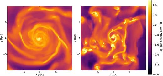
Face-on mass-weighted mean gas density maps of the isolated runs: gp-iso is shown on the left-hand panel and iso on the right-hand panel. Both maps are obtained after an evolution during the time corresponding to the first pericentre for orbit #1 (490 Myr after the start of the simulation).
In Fig. 2, we show the gas density map of the merger in the low and high gas fraction case for orbit #1 (dd1 and gp-dd1) at different times of the interaction; a few 10 Myr before and after both the first pericentre passage and the coalescence. We see that the gas in the low gas fraction case shows the formation of a few clumps in the tidal bridge after the first pericentre passage. On the bottom row, the evolution of the gas density of the high gas fraction case does not show any significant increase in the number of clumps before and after the first pericentre passage.
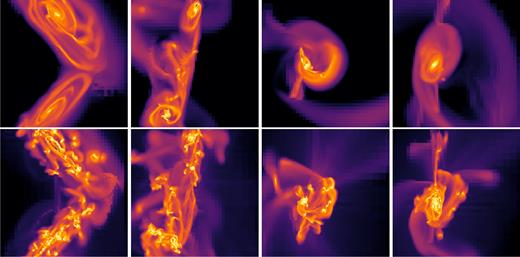
Mass-weighted mean gas density map of the gas-poor (top panel) and gas-rich (bottom panel) simulations for the direct–direct interaction orbit #1 at different times from the first pericentre : −60, 105, 370, and 560 Myr from left to right. The maps span an area of 30 kpc × 30 kpc. The colour scale is the same as in Fig. 1.
To have a more quantitative insight into the interaction-driven clumpiness of the disc, we use the friend-of-friend algorithm HOP (Eisenstein & Hut 1998) to determine the number of clumps and the gas mass fraction embedded in them, during the interaction. Clumps are detected around peaks of gas density above 40 cm−3. Subclumps are merged if the saddle density between them exceeds 4 cm−3 and an outer boundary of 2 cm−3 is set to define the density limit of the clumps. These parameters agree with a visual examination of the density maps and the results are not affected with respect to small changes of these parameters.
In Fig. 3, we show the evolution of the number of clumps, and the gas fraction inside them. In the low gas fraction case, the gas fraction enclosed in clumps goes from 5 to 25 per cent at the first pericentre passage, and the number of clumps increases by a factor of 4, from about 4 to 16. These numbers stay relatively constant along the interaction. This enhanced number of clumps in low-redshift galaxy collisions has been already noted by Di Matteo et al. (2008). In the high gas fraction case, the gas mass fraction in clumps shows instead a slow but steady decrease of both the number of clumps and gas mass fraction enclosed. The evolution of the number of clumps and masses of the high gas fraction case are therefore not influenced by the interaction as we can see by comparing the isolated (iso) and the interacting cases (dd1). In particular, no change is observed at the first pericentre passage.
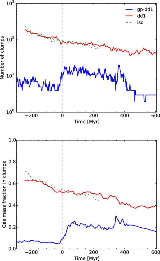
Top: number of detected clumps for the low (blue) and high (red) gas fraction for dd1 and gp-dd1. The isolated run for the high gas fraction case is also shown in dashed green. To ease the comparison, this number is multiplied by 2 for the isolated case. Bottom: gas mass fraction in gas clumps.
3.2 Evolution of the density PDF
In the low gas fraction, this interaction-induced clumpiness condensates the gas in localized over densities. To quantify its effect on the gas density distribution, we look at the evolution of the mass-weighted density probability density function (PDF). In Fig. 4, we see the evolution of the shape of the gas PDF for both the low and high gas fraction cases. In the low gas fraction case, the PDF extends to higher densities during the interaction. We also see that the PDF of the high gas fraction case remains almost identical during the interaction and does not significantly vary from the shape of the isolated galaxy PDF, except at the coalescence (t = 376 Myr) where there is an increase of the mass with densities above 3 × 104 cm−3.
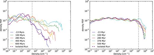
Normalized mass-weighted probability distribution function of the gas density, at several epochs (t = 0 corresponds to the first pericentre). These times correspond to before the first pericentre, shortly after the first pericentre, before the coalescence, peak of SFR during coalescence, long after the coalescence, respectively. Curves are shown for the direct–direct encounter on orbit #1 for the low (left) and high (right) gas fraction cases in solid lines. The thick purple lines show the corresponding isolated cases. The black dashed line indicates the density threshold for star formation as defined in Section 2.1.
The evolution of the shape of the PDF is of particular interest, as high-density gas fuels star formation. Indeed, in the low gas fraction case, the gas mass above the density threshold goes from 4 to 20 per cent after the first pericentre passage and 40 per cent at the coalescence, while it stays constant, at 2–3 per cent, in the high gas fraction case.
3.3 Merger-induced star formation
3.3.1 Star formation histories
The comparison between low and high gas fraction star formation histories during the interaction is shown in Fig. 5. In the low gas fraction case, the SFR is about 1–2 M⊙ yr−1 before the interaction and increases to ∼30 M⊙ yr−1 and more than 50 M⊙ yr−1 after the first pericentre passage. The SFR then lowers back to a few M⊙ yr−1 before increasing again to ∼40–60 M⊙ yr−1 during the final coalescence.
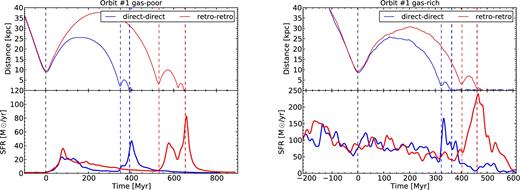
SFR during the simulations run on orbit #1, with the distance between the galaxies plotted above. The direct–direct and retro–retro simulations are shown, respectively, in blue and red. The low gas fraction case is shown on the left-hand panel and the high gas fraction case on the right-hand panel. The dashed lines correspond to the time of the first pericentre passage (in black) and the respective times of second pericentre passage and coalescence (in the colour corresponding to the simulation).
The high gas fraction case shows a very different history. The SFR is initially relatively high, ≃120 M⊙ yr−1 for the galaxy pair, and does not increase significantly at the first pericentre passage. The SFR is only enhanced at the coalescence,4 and only by a factor at most 5. Increasing only the gas fraction thus appears to significantly lower the boost of SFR.
To ensure that this results does not depend on a particularity of the chosen orbit or orientation, we also look at the SFR of the two other tested orbits and orientations, which are displayed in Fig. 6. We see that they follow the behaviour of orbit #1; they all show almost no increase of star formation at the first pericentre passage, and a mild burst at coalescence.

3.3.2 The starburst sequence
Our motivation to run these simulations resides in the fact that a smaller than expected number of high-redshift galaxies are found on the starburst sequence of both the M⋆–SFR and Σgas–ΣSFR diagrams, the latter being also known as the Schmidt–Kennicutt diagram.
In Fig. 7, we can see the evolution of our simulated galaxies on the Schmidt–Kennicutt diagram. The computation is done in a box of 60 kpc×60 kpc×60 kpc and we rescale the curves so that the pre-merger discs lie on the disc sequence. To better quantify the starbursting behaviour of our simulations, we define the starburstiness parameter as the measured ΣSFR over the value of ΣSFR corresponding to the disc sequence of Genzel et al. (2010) for the measured Σgas. We define starbursting galaxies as galaxies with a starburstiness exeeding 4, meaning that they stand more than 0.6 dex above the disc sequence, which is a common definition for the starburst sequence (Schreiber et al. 2015).

Top panel: evolution of the simulations dd1 (shades of blue) and rr1 (shades of red) on the Schmidt–Kennicutt diagram. The solid lines show the high gas fraction cases, and the dotted lines the low gas fraction cases. The red dots and stars show, respectively, the time of the first and second pericentres. The solid and dashed black lines are, respectively, the disc and starburst sequences from Genzel et al. (2010). The curve is smoothed using a constant kernel on the previous 100 Myr, to resemble the smoothing of the measurements of the SFR using IR luminosity (Kennicutt 1998). Bottom panel: evolution of the starburstiness, as defined in the text, during the interaction. The colours and labels are the same as in the upper panel. The black solid line indicates a starburstiness of unity, i.e. an SFR equivalent to the disc sequence for a given, Σgas, and the dotted line shows a starburstiness of 4, which we define as the lower limit to be considered as a starburst galaxy.
We see that the galaxies follow the disc sequence until the collision which shifts their loci towards the starburst sequence. The low gas fraction systems reach the starburst sequence already at the first pericentre passage and their starburstiness stays above 4 all along the starburst, that is for more than 700 Myr for the considered orbit. The high gas fraction pairs hardly reach the starburst sequence: the gas-rich direct–direct starburstiness always stays below 4 and is thus never considered as a starburst galaxy. The burst at the coalescence of the gas-rich retrograde–retrograde encounter makes it reach the starburst sequence of the Schmidt–Kennicutt diagram, but only for ∼100 Myr.
In the following, we analyse the processes that influence the ability of high fraction gas merger to trigger starbursts, as compared to low gas fraction ones.
4 WHAT CAUSES THIS WEAK ENHANCEMENT OF STAR FORMATION?
4.1 Weak increase of the central gas inflows
Observed starbursting galaxies show a prominent nuclear starburst (Sanders & Mirabel 1996), with an important concentration of gas in the central kpc of the galaxies. Fig. 8 shows the fraction of SFR located in the central kpc of the galaxies. We see that at the coalescence, the peak of star formation is almost entirely located in this central kpc.5
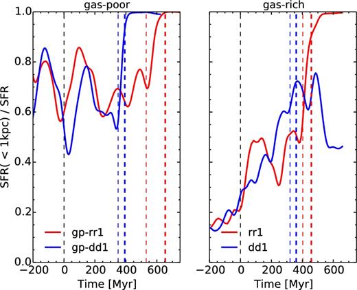
Evolution of the fraction of SFR located inside the central kpc of both galaxies for the encounters on orbit #1 in the low gas fraction case (left) and high gas fraction cases (right). The vertical dashed lines are the same as in Fig. 5.
This centrally concentrated star formation is fuelled by gas inflows towards the centre. Interaction-driven gravitational torques are indeed expected to drive a large amount of gas towards the nuclei of both galaxies (Barnes & Hernquist 1991; Mihos & Hernquist 1996). In Fig. 9, we show the inflows of baryonic mass in the central kpc of our galaxies. For the low gas fraction case, pre-merger discs have central mass inflows of ≃2–3 M⊙ yr−1. Between the first and second pericentre, the discs are perturbed and the inflows have a higher mean value of about 20 M⊙ yr−1, with some important variation over time. At coalescence, the inflows reach a peak at 20 M⊙ yr−1 for the dd1 and 50 M⊙ yr−1 for the rr1 simulation, which are both at least 10 times higher than the initial gas inflows in the isolated case.
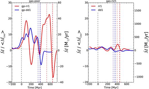
Evolution of the inflow of baryonic mass fraction in the central kpc of both galaxies for the encounters on orbit #1 in the low gas fraction case (left) and high gas fraction case (right). The left axis shows the ratio of the inflow to the mean inflow rate of the isolated run, and the same scale is used for both plots to emphasize the relative difference to the isolated case. The right axis shows the actual value of the inflow rate. The curves are smoothed using a Gaussian kernel of root-mean-square width 30 Myr for the sake of clarity. The vertical dashed lines are the same as in Fig. 5.
For the high gas fraction case, the central inflows are stronger from the beginning, ≃30–50 M⊙ yr−1. As in the low gas fraction case, a strong peak in inflows is seen for the rr1 simulation, at 250 M⊙ yr−1. The relative increase compared to the pre-merger case is less than 5, much less than for the low gas fraction case. The resulting increase in SFR is also comparatively less important than for the low gas fraction case.
Central gas inflows are already strong in the pre-merger high gas fraction disc because of the VDI; the high turbulence of the gas is in part fuelled inwards by the migration of gas (Dekel, Sari & Ceverino 2009b). Another physical explanation for the higher increase of the central inflows in low gas fraction discs is the presence of a more massive stellar component which creates a tidally induced bar or spiral arms which exert strong torques on the gas, and which adds to the effect of the gravitational torques originating from the companion. The stellar component being less populated in the high gas fraction case, this process is less efficient, as already noted by Hopkins et al. (2009).
The high gas fraction, which leads to a high turbulence and the formation of clumps, also drives strong gas inflows in the isolated discs. As a result, interaction-induced gas inflows are less important with respect to pre-merger inflows for high gas fraction discs than for low gas fraction discs. This leads to a lower increase of SFR due to central gas inflows.
4.2 Mild enhancement of gas turbulence
Our current understanding of extended starburst in low gas fraction galaxy interactions is that the increase of the SFR is caused by an increase of gas turbulence.
We compute the one-dimensional velocity dispersion of the gas, along the line of sight of the simulations at the scale of 100 pc and plot its evolution in Fig. 10. We see that the pre-interaction velocity dispersion is much higher in the high gas fraction case, σ ≃ 35 km s−1, than in the low gas fraction case, σ ≃ 10 km s−1. This agrees with observations (Förster Schreiber et al. 2009) and is due to the gas phase which is more gravitationally unstable with high gas fraction. The interaction brings the velocity dispersion of the low gas fraction case to more than 40 km s−1, in agreement with both observations (Elmegreen et al. 1995, 2016a) and previous simulations (Bournaud, Duc & Emsellem 2008, R14). In the high gas fraction case, the velocity dispersion goes up to around 60 km s−1 only. The relative increase in turbulence is much higher in the low gas fraction case, a factor of 5, to be compared to the high gas fraction case, which shows an increase of less than a factor of 2.
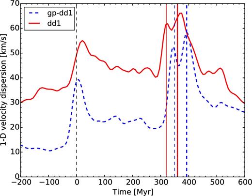
Evolution of the gas velocity dispersion of the direct–direct simulations on orbit #1. The low gas fraction is depicted by the blue dashed curve and the high gas fraction by the solid red line. The vertical dashed lines are the same as in Fig. 5.
This heuristic calculation shows the difficulty of increasing the velocity dispersion while it is already high, which leads to a mild increase in gas turbulence from interactions in high gas fraction discs.
4.3 Absence of interaction-induced tidal compression
The increase in compressive turbulence is thought to be driven by the onset of fully compressive tides (see R14). On top of triggering compressive turbulence, fully compressive tides also reduce the Jeans mass and help gas fragmentation in star-forming clumps (Jog 2013, 2014). Extended regions undergoing fully compressive tides are a common feature of galaxy encounters (Renaud et al. 2008, 2009).
To measure the impact of compressive tides on our galaxies, we compute the tidal tensor defined by its components Tij = −∂i∂jϕ using first-order finite differences of the total gravitational force at the scale of 50 pc. The tidal field is compressive if the maximum eigenvalue of the tensor is negative. The method is the same as R14. Results for the low and high gas fraction runs on the Orbit #1 are shown on Fig. 11.
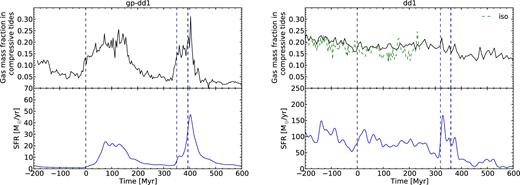
Evolution of the gas mass fraction in a fully compressive tidal field (top panel) compared to the SFR (bottom panel) for the direct–direct encounter on orbit #1 in the low gas fraction case (left) and high gas fraction case (right). The vertical dashed lines are the same as in Fig. 5.
We see that, in the low gas fraction case, the gas mass fraction in compressive tides increases from 7 to 20 per cent during the pericentre passages. These values are similar to those obtained in previous simulations of galaxy interactions (using N-body; Renaud et al. 2008, 2009, using AMR; R14).
In the high gas fraction case, the mass gas fraction in compressive tides is initially higher and tend to slowly and monotically decrease with time, with no significant changes induced by the pericentre passages.
This high but steady gas mass fraction in compressive tides results from the matter distribution of the galaxy. In Fig. 12, we show the position of tidally compressive regions ≃60 Myr after the first pericentre passage. In the low gas fraction case, we see that tidally compressive regions develop over extended regions close to the galaxy nuclei, in the forming tidal tails and in the bridges between the two galaxies. In the high gas fraction case, the tidally compressive regions are mainly located inside the clumps. The gravitational potential is locally dominated by the highly concentrated clumps (see Section 3.1), leaving the interclump medium in tidally extensive zones which makes the formation of any zone of compressive tides harder, and limits any increase in gas fragmentation during the interaction.
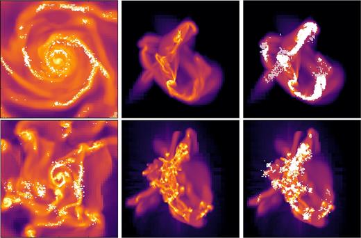
Gas density maps for the gas-poor (top panel) and gas-rich (bottom panel) simulations. The left-hand panels show the isolated galaxies. The central and right-hand panels show the direct–direct interaction for orbit #1 at t = 60 Myr. The maps span 10 kpc × 10 kpc for the isolated runs and 50 kpc × 50 kpc for the merger runs. The colour map is the same as in Fig. 1. The white dots in the left- and right-hand columns show the location of the tidally compressive regions.
This adds to the small enhancement of the turbulence, described in Section 4.2, which limits an increase in compressive turbulence, and thus a change in the density PDF and in the interaction-induced SFR.
In summary, our numerical simulations show that the clumpy nature driven by the high gas fraction has a strong influence on the central inflows, the gas turbulence and the compressive tides. These three physical processes are seen to be enhanced during low-redshift encounters and are thought to be responsible for the interaction-driven starburst in low-redshift galaxies. In the high gas fraction cases, these three processes are already strong in isolated galaxies and are not further enhanced by interactions.
Our simulations hereby confirm the importance of these three processes in the increase of the SFR in gas-poor interactions and we claim that their weak enhancement for high gas fraction discs explains the relative diminished efficiency of gas-rich major mergers to trigger starbursts.
4.4 No effect of saturation from feedback
The SFR of the high gas fraction discs in isolation is ≃60 times higher than that for the low gas fraction discs, the net feedback energy from SNe explosions and H ii regions is therefore also much higher. One can wonder whether an increase of star formation is not self-regulated in high gas fraction discs because of the stellar feedback.
To test this hypothesis, we restart the dd1 simulations, but with all sources of feedback, which were presented in Section 2.1, turned off. One should note that an absence of feedback for a long period of time would transform significantly the structure of the galaxies, as stellar feedback regulates the growth of gas clumps (Bournaud et al. 2010; Hopkins, Quataert & Murray 2011; Goldbaum, Krumholz & Forbes 2016). Shutting off feedback just before the investigated event, i.e. the galactic encounters, ensures that we compare galaxies with the most similar structure as possible. Therefore, we shut off the feedback around 40 Myr only before the two moments when a rise of SFR is expected, namely the first pericentre passage and the coalescence. The time-scale of dissipation of the turbulence being around 10 Myr (Mac Low 1999) at the clumps scale, which is comparable to the free-fall time, we ensure that there is no more influence of the feedback on the gas turbulence at the expected starburst time.
The evolution of the SFR for the feedback case and no-feedback case is plotted in Fig. 13. We see that there is a small increase in SFR, especially at coalescence, in the simulations without feedback, but the general behaviour does not change; even without stellar feedback, the interaction only induces a small starburst compared to the low gas fraction case. This weak influence of feedback on high gas fraction major mergers has already been seen in Bournaud et al. (2011) and Powell et al. (2013).
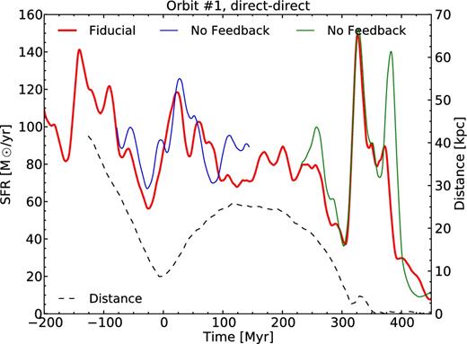
Evolution of the SFR for the dd1 simulation and runs with turned off stellar feedback at different times. The red solid line shows the SFR of the fiducial run, dd1, presented in Fig. 5. The blue and green lines show the SFR resulting from the runs without feedback. They separate from the fiducial curve slightly before the time delay indicated in the text because of the curve smoothing. The black dashed line shows the distance between the two galaxies.
Our simulations show that our feedback implementation, which allows a burst of star formation for low gas fraction major mergers, is not responsible for the weakness of the star formation enhancement in the high gas fraction case. The implementation of subgrid models of stellar feedback in numerical simulations is a long-standing issue. Energy outputs from SNe and stellar winds are theoretically rather well understood for most stellar populations (see the review by Dale 2015), but the details in the numerical implementations are important and can lead to significantly different results (see e.g. Hopkins, Quataert & Murray 2012; Agertz et al. 2013). A detailed study of the impact of the implementation of feedback on galaxy structure is beyond the scope of this paper.
On the one hand, our no-feedback simulations show that a weaker feedback than ours would not produce a strong enhancement of star formation either. On the other hand, a stronger feedback would increase the pre-interaction overall gas turbulence. As we have seen in Section 4.2, the interaction-induced increase of turbulence would be even smaller which would lead to an even weaker enhancement of the SFR. This shows that the weakness of merger-driven starbursts at high redshift (compared to low-redshift cases) does not result from saturation by feedback in our models, and this result could only be stronger if real feedback had more important effects in high-redshift galaxies.
5 DISCUSSION
5.1 Comparison with previous simulations
Our simulations show that the high gas fraction major mergers are less efficient than low gas fraction major mergers to trigger starbursts. Here, we compare our results to previous studies of clumpy gas-rich major mergers.
The first simulations of gas-rich (fgas > 50 per cent) galaxy mergers could not resolve the impact of turbulence on star formation (Springel & Hernquist 2005; Cox et al. 2006; Hopkins et al. 2006; Lotz et al. 2008; Moster et al. 2011); their discs are less unstable than ours and tend to form spirals instead of clumps. They resolve the star formation enhancement due to the increase of nuclear inflows through interaction-driven gravitational torques, but miss the increase of gas fragmentation and the initial, clump-driven, nuclear inflows, which make them to overestimate the relative increase of SFR.
Bournaud et al. (2011) have run the first numerical simulations of gas-rich clumpy galaxies. On their three orbits, they saw an increase of the SFR of up to a factor of 10 (from 200 M⊙ yr−1 to peaks of 2000 M⊙ yr−1) for more than 200 Myr. It results in a higher increase of SFR than in our sample, but still below usual low gas fraction major mergers. One should note that they do not use a cooling function, but a barotropic equation of state (presented in Bournaud et al. 2010), which tends to overestimate the gas fragmentation.
Hopkins et al. (2013) present a suite of parsec-resolution galaxy collision simulations, with one high-redshift-type galaxy major merger (fgas = 50 per cent) and a feedback implementation which systematically destroys gaseous clumps. Their fig. 9 shows that the enhancement of star formation is indeed significantly smaller and has a ≃10 times shorter relative amplitude than their Milky Way-type galaxy major merger. Their starburst duration is similar to that obtained in our simulations: ∼100 Myr and ∼1 Gyr for, respectively, the high and low gas fraction cases. They did not study this weak enhancement in details, as they changed several parameters between the low- and high-redshift runs (halo mass, the disc compactness and velocity profile).
In the merger sample of Perret et al. (2014), no simulation shows any increase of the star formation during the interaction. They stressed that one explanation for this could be due to their implementation of feedback; they set a density-independent cooling time for the gas heated by the SNe of 2 Myr, which prevents very dense region in star-forming regions to form stars again during this time. One should note that they did not test their feedback on low gas fraction major mergers, contrary to the present study, so that it is uncertain whether this implementation would allow them to trigger starbursts in low-redshift conditions.
The fact that high gas fraction major mergers trigger a smaller enhancement of star formation than their low gas fraction equivalent was already seen in previous studies, using various numerical methods and feedback implementations. With this suite of simulations, we propose that the variation in gas fraction only can explain the mildness of this enhancement.
5.2 The cosmological context
5.2.1 Gas refuelling
Our galaxy pairs are not refuelled by cosmological gas infall. The presence of cosmological cold gas infall on galaxies, inferred from cosmological simulations (Dekel et al. 2009a,b) but not yet observed, is thought to be the main channel of galaxy mass growth at high redshift, when major mergers would contribute to only one-third of the mass growth (Kereš et al. 2005; Ocvirk, Pichon & Teyssier 2008; Brooks et al. 2009).
Even though no cosmological infall is considered in our work, the galaxies are initially located in a box with an intergalactic medium (IGM) of background density 2 × 10⁻⁷ cm−3. This gas can cool down and contribute to the baryonic mass budget of the galactic discs.
In the top panel of Fig. 14 is shown the quantity of baryonic matter in the galaxies (stars and gas above 10−2 cm−3), normalized to the initial baryonic mass of two times 57.2 × 10⁹ M⊙ (see Table 1). We see that the baryonic mass of the galaxy pair does not change by more than 4 per cent throughout the simulations. These variations are either due to stellar outflows, which can bring some gas to densities lower than our threshold of 10−2 cm−3, or due to the cooling of the IGM gas on to the disc. We see that these two processes do not affect our mass budget.
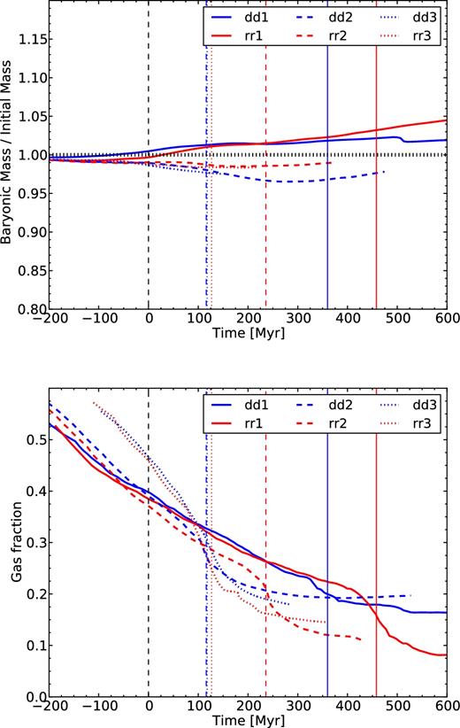
Top: amount of baryonic matter (Mgas + Mstars) renormalized to the initial baryonic mass: 2 × 57.2 × 109 M⊙ (see Table 1). The vertical dotted line shows a ratio of 1. Bottom: gas fraction evolution during the simulation for six gas-rich orbits. For both panels, only gas with density above 10−2 cm−3 is considered, in order to only count the gas present in the galaxies. All curves are shifted in time, such that t = 0 is the time of first pericentre for each orbit. The small coloured vertical lines show the time of coalescence for each orbit, as labelled in the legend.
A first drawback of not adding gas accretion in our simulations is that the cold gas mass reservoir available to form stars is not replenished by these cold flows. For instance, in our two simulations on orbit #1 – the less bound one for which coalescence happens after more than 300 Myr from the first pericentre – the long-term evolution of the SFR in Fig. 6 is seen to be slowly decreasing, as a consequence of gas consumption.
In the bottom panel of Fig. 14 is shown the gas fraction evolution during the gas-rich simulations on orbits #1, 2 and 3. We see that the gas is steadily consumed before the first pericentre, at t = 0, where the gas fraction is still at around 40 per cent or more. Before the coalescence, the gas fraction is above 25 per cent for orbits #1 and 2, and above 40 per cent for the faster orbit #3. Just before coalescence, the faster gas consumption through star formation leads to a rapid drop in the gas fraction.
We see that for orbit #3, the effect of gas consumption is relatively weak as the gas fraction is still above 40 per cent at the time of the coalescence. The fact that the SFR for these orbits do not show much difference in behaviour from orbit #1 comforts us in concluding that this would not have an important effect on the SFR of our simulations.
However, on longer time-scale, gas accretion would impact the star formation in the merger remnant. Indeed, in Fig. 7, we see that after the coalescence, the SFR of the gas-rich merger drops well below what is expected from the remaining gas fraction. This is due to the formation of a massive stellar spheroid, dispersion-dominated, which stabilizes the gas and prevent it to form stars. This process is called morphological quenching (Martig et al. 2009). Recent simulations of high gas fraction galaxies surrounded by hot gaseous haloes, presented by Athanassoula et al. (2016), show that a disc of gas can form through gas accretion inside the spheroid core. This disc will be bar-unstable and form stars.
At z = 2, the mass inflow from cosmological accretion is of the order of 10 M⊙ yr−1 (Dekel et al. 2009a). Martig et al. (2009) have shown that, with this accretion rate order of magnitude and without any other merging event, several gigayears are necessary to reform a star-forming disc in a spheroidal major merger remnant, which is the same order of magnitude of formation of a disc found by Athanassoula et al. (2016).
5.2.2 Turbulence from cosmological infall
A second effect is that we neglect the increase of turbulence from the cosmological accretion. The infalling gas does not settle immediately into a thin disc but tends to stir the existing gas disc (Elmegreen & Burkert 2010; Gabor & Bournaud 2014), which has for net effect to increase the velocity dispersion and the disc height. The SFR is thought to be regulated by this constant fuelling of turbulence on to the disc, until z = 2 when this process stops dominating the turbulence budget (Gabor & Bournaud 2014).
In Section 4.2, we claim that the merger does not increase the turbulence, because it is already high. Turbulence pumped through cosmological infall would make it even harder for the interaction to further increase the turbulence. Therefore, we argue that this process would not change our conclusions.
5.2.3 Galaxy compactness and orbits
A last effect is that high-redshift galaxies are more compact than low-redshift galaxies, for the same mass, typically a factor ≃2 (van der Wel et al. 2014; Ribeiro et al. 2016). In this study, we neglect this effect to focus on the difference in gas fraction only. However, our galaxy model has an intermediate compactness, between low and high redshift conditions.
Furthermore, for equal halo mass, cosmological simulations expect the pericentre distance to be 25 per cent lower at z = 2 than at z = 0 (Wetzel 2011). All dynamical time-scales are then shorter and the merging process is faster. This could result in more starburst-favourable orbits.
Orbit #2 (resp. #3) has impact parameter and relative velocity, respectively, 15 per cent (resp. 30 per cent) lower than orbit #1, which makes it closer to typical z = 2 orbits. We see in Fig. 6 that these three orbits share a comparable increase in SFR. This hints for a low dependence of the orbit parameter on the weakness of the interaction-driven star formation in high gas fraction discs.
5.3 Application to local gas-rich dwarf galaxies interactions
Local dwarf irregulars (dIrrs) have fgas up to 90 per cent, contain clumps and are relatively turbulent with a ratio of their circular velocity to velocity dispersion, Vcirc/σ, around 6 (see e.g. Lelli, Verheijen & Fraternali 2014, and references therein), which is of the same order than massive high-redshift galaxies. Our reasoning, which is based on the high gas fraction and highly turbulent high-redshift galaxies, might thus also apply to dIrrs. However, Stierwalt et al. (2015) recently claimed that interactions between dIrrs can significantly increase their SFR, that is more than five times above the MS.
It should be noted that, if the gas fraction of dIrrs is very high, it is mainly due to a diffuse H i envelope, which does not participate actively to the star formation. This envelope can however cool and be accreted on to the central region (see e.g. Elmegreen et al. 2016b).
A second important difference with respect to high-redshift massive galaxies is that isolated dIrrs do not show signs of instability-driven inflows, as they do not have important nuclear concentration. For the gas to be funnelled towards the nucleus, the work of the gravitational torques from the gaseous clumps, which scale with their mass (Mclump), must compensate the galactic rotational kinetic energy of the gas ∝ vcirc2, which results in an inflow time-scale ∝ vcirc2/Mclump.
Both dIrrs and high-redshift massive galaxies show clumps of typical masses of a few per cent of the galaxy mass, that is ≃107 M⊙ (Elmegreen, Zhang & Hunter 2012), and rotation velocities of about 50 km s−1 (Lelli et al. 2014), against 109 M⊙ clumps (Elmegreen et al. 2009) and 200 km s−1 rotation velocities for massive high-redshift galaxies. The inflow time-scale is then a factor of 6 longer for dIrrs. The fact that the relative torquing of the gas is much less efficient in dIrrs makes the central inflows driven by the interaction between dIrrs relatively more important and can thus more easily ignite a starburst.
The more diffuse location of the gas in dIrrs and the low efficiency of instability-driven central inflows therefore limit the extension of our results from massive high-redshift galaxies to dIrrs.
5.4 Starbursting galaxies observed at high redshift
In Figs 5 and 6, we see that interactions do not strongly enhance the SFR of high gas fraction galaxies: from around 120 M⊙ yr−1 (60 M⊙ yr−1 for each galaxy), our most actively star-forming galaxy barely reaches 350 M⊙ yr−1 during 50 Myr. Observations of submillimetre galaxies (SMGs) report SFRs up to several 1000 M⊙ yr−1 (Barger et al. 1998; Tacconi et al. 2006). Observed SMGs are found on both the MS and the starburst sequence of the M⋆–SFR (da Cunha et al. 2015). There are also claims that SMGs form the high-mass end of the MS (Koprowski et al. 2016; Michałowski et al. 2016).
Recent numerical simulations presented in Narayanan et al. (2015) show that the regime of SMGs galaxies can be achieved without major mergers, but rather by continuous gas infall through accretion of small haloes on to a very massive group halo (≃1013 M⊙) which may be populated by several galaxies. On top of that, Wang et al. (2011) show that the relatively high abundance of SMGs might result from the blending of sources that are not necessarily spatially associated, which agrees with a not high enough number of major merger to account for the observed SMG abundance (Davé et al. 2010).
These studies do not exclude major mergers as being a cause of a part of the observed SMGs. However, one should note that the progenitors of such galaxies are significantly more massive than our simulated discs (M⋆ ≃ 1011 M⊙), i.e. five times higher than our galaxy models. Therefore, we cannot conclude on the possibility of part of the SMGs being triggered by high-redshift major mergers.
6 CONCLUSIONS
Observations of star-forming galaxies over a wide range of redshifts (z = 4–0) have shown a MS on the M⋆–SFR relation, with a number of outliers galaxies showing a higher specific SFR, which correspond to the starbursting galaxies. The proportion of these outliers stays relatively constant (≃2 per cent) with time, with no clear dependence with redshift. In the local Universe, all these outliers are merging galaxies. Since the merger rate is thought to increase with redshift, high-redshift major mergers seem to be less efficient to produce starbursting galaxies than low-redshift ones. We present a suite of parsec-resolution hydrodynamical simulations to test this hypothesis. We have run simulations of typical low- and high-redshift galaxy pairs, changing only the gas fraction, from 10 to 60 per cent, between the two models.
We see that for the same orbit, when the SFR of the low gas fraction goes up by a factor of more than 10 during several hundred million years, the SFR of the high gas fraction case only mildly increases, and only at the coalescence. In particular, we show that the high-redshift-type galaxies would not, or for a short amount of time (≃50 Myr), be considered as starburst galaxies on a Schmidt–Kennicutt diagram.
Even in the absence of stellar feedback, no higher burst of star formation is seen. We reject feedback saturation as a cause to the inefficiency of the interaction to trigger a strong enhancement of star formation.
At coalescence, most of the star formation happens in the central region of both galaxies, typically in the central kpc. This starburst is fuelled by central mass inflows caused by the interaction, which add up to the mass inflow processes already at play in the isolated discs. This makes the coalescence phase less efficient in triggering a starbursting galaxy in the high gas fraction case than the low gas fraction case.
R14 have shown a correlation between the increase in compressive turbulence and the onset of the interaction-driven starbursting mode of star formation. Our high-redshift-type galaxy interactions show only a mild increase of turbulence. High gas fraction clumpy discs are already quite turbulent (σ ≃ 40 km s−1) and it is harder to increase the velocity dispersion through release of gravitational energy when the initial velocity dispersion is already high.
On top of this smaller increase of the gas turbulence, the clumpy morphology also imposes an extensive tidal field on the interclump regions. These two processes limit the increase in compressive turbulence, and thus the increase in SFR during the interaction.
This demonstrates that the high gas fraction of the galaxy progenitors can strongly reduce the star formation enhancement in galaxy interactions and major mergers.
Acknowledgments
The authors thank Vianney Lebouteiller and Damien Chapon for very useful discussion and the anonymous referee for constructive comments which helped to improve this paper. Simulations were performed at TGCC (France) and as part of a PRACE project (grant ra2540, PI: FR) and GENCI project (grant gen2192, PI: FB). FR acknowledges support from the European Research Council through grant ERC-StG-335936.
We use the same metallicity for both high- and low-redshift galaxy models as an approximation to investigate the effects imputable to the variation of gas fraction only. Massive high-redshift galaxies can have a metallicity up to half-solar (see e.g. Erb et al. 2006).
See movie at https://www.youtube.com/watch?v=ByV1g24eEjk
In both gas fraction cases, the retrograde–retrograde simulation coalescence happens later than in the direct–direct simulation. This is expected because they do not form tidal tails, which are efficient in driving angular momentum out.
With the exception of dd1 simulation; in Fig. 2, one can actually see in the bottom-right corner that this particular simulation forms an irregular fragmented structure, surrounded by dense, star-forming gas clumps more than 1 kpc away from the centre, which explains why star formation is not confined in the central kpc only.
REFERENCES
APPENDIX A: STUDY OF SPATIAL RESOLUTION
In order to test the impact of the resolution on star formation of our high-redshift simulations, we run the dd1 simulation with different resolution both in space and in mass.
In the upper panel of Fig. A1 is shown the SFR for the dd1 simulations for different highest spatial resolution, from 50 to 6 pc. In the lower panel of Fig. A1 is shown the SFR for the dd1 simulations for different highest spatial resolution, using a different mass resolution. For the two new refinement simulations, the mass needed to activate the next refinement level was divided by 8 for cells smaller than 100 pc. Therefore, all cells that were refined to 50 pc in the non-new refinement simulations are directly refined to 25 pc in the new refinement case, and so on for further refined cells.
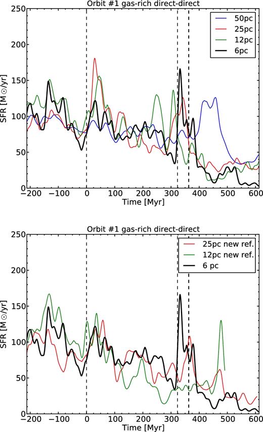
Top: SFR during the interaction for the dd1 simulation at different maximum spatial resolution. Bottom: same as in the top panel, with a different refinement strategy for the new refinement labelled simulations. The black dotted lines show the time of pericentre passages and coalescence of the dd1 simulation at 6 pc resolution.
The stochasticity of the SFR and the fact that each simulation is run with a different ρ0 calibration induce some variations in the pre-merger SFR. The time of the final coalescence can change with the resolution as the resolution will impact several processes governing the interaction. For instance, another resolution can modify how the angular momentum is driven out of the inner system through the tidal tails and/or impact the dynamical friction.
In Fig. A1, there appears to be no significative trend with the resolution. In particular, no simulations show any onset of a massive star formation burst during the interaction. We therefore see that the resolution has little influence on the evolution of the SFR during the interaction, which legitimates our use of a resolution of only 12 pc for the simulations run with Orbits #2 and #3.
