


Abstract
We study the properties of gas in and around 1012 M⊙ haloes at z = 2 using a suite of high-resolution cosmological hydrodynamic ‘zoom’ simulations. We quantify the thermal and dynamical structure of these gaseous reservoirs in terms of their mean radial distributions and angular variability along different sightlines. With each halo simulated at three levels of increasing resolution, the highest reaching a baryon mass resolution of ∼10 000 solar masses, we study the interface between filamentary inflow and the quasi-static hot halo atmosphere. We highlight the discrepancy between the spatial resolution available in the halo gas as opposed to within the galaxy itself, and find that stream morphologies become increasingly complex at higher resolution, with large coherent flows revealing density and temperature structure at progressively smaller scales. Moreover, multiple gas components co-exist at the same radius within the halo, making radially averaged analyses misleading. This is particularly true where the hot, quasi-static, high entropy halo atmosphere interacts with cold, rapidly inflowing, low entropy accretion. Haloes at this mass have a well-defined virial shock, associated with a sharp jump in temperature and entropy at ≳ 1.25 rvir. The presence, radius, and radial width of this boundary feature, however, vary not only from halo to halo, but also as a function of angular direction, covering roughly ∼75 per cent of the 4π sphere. We investigate the process of gas virialization as imprinted in the halo structure, and discuss different modes for the accretion of gas from the intergalactic medium.
1 INTRODUCTION
Initially following the gravitational collapse of a dark matter overdensity, gaseous haloes subsequently grow through the accretion of baryons from the intergalactic medium (IGM). Their evolving structure across cosmic time has been the subject of theoretical as well as observational interest for several decades. As the transitional state between the diffuse IGM and the star-forming interstellar medium (ISM) of galaxies, these gas reservoirs regulate the stellar growth of forming galaxies. Understanding not only the structure of halo gas, but also its origin and subsequent evolution, is therefore essential for any comprehensive theory of galaxy formation.
Although the accretion of gas will follow that of dark matter, the presence of additional physical processes including hydrodynamical forces and radiative cooling imply additional complexity for the acquisition of baryons. In the classic picture, gas accreting from the IGM will shock heat to the virial temperature of the halo. If the radiative cooling time-scale is sufficiently long, it will then form a hot, pressure supported atmosphere in approximate equilibrium (Rees & Ostriker 1977; Silk 1977; White & Rees 1978). Cooling can proceed, delivering gas into the halo centre (White & Frenk 1991). For sufficiently low-mass haloes, this time-scale will be short enough that a ‘stable virial shock’ cannot develop, and gas accretion from the IGM will proceed as rapidly as dynamically allowed (Birnboim & Dekel 2003). However, this theoretical foundation is largely based on a one-dimensional picture, while dark matter haloes and their gaseous counterparts are decidedly not spherically symmetric. Numerical hydrodynamical simulations have indicated that galaxies can acquire their gas in a fundamentally different manner (Abadi et al. 2003; Katz et al. 2003; Kereš et al. 2005; Ocvirk, Pichon & Teyssier 2008). In particular, finding that coherent, filamentary inflows can fuel star formation in a central galaxy while avoiding shock heating to the virial temperature. Such streams arise naturally from the topology of large-scale structure, particularly at high redshifts of z ≳ 2 (Agertz, Teyssier & Moore 2009; Dekel et al. 2009; Kereš et al. 2009; Danovich et al. 2012).
Gas inflow has been studied in the context of many key theoretical questions in galaxy formation, most fundamental of which are perhaps its link to star formation (Dekel et al. 2009, 2013; Oppenheimer et al. 2010; Gabor & Bournaud 2014; Sánchez Almeida et al. 2014) and the process of quenching (Birnboim & Dekel 2003; Birnboim, Dekel & Neistein 2007; Gabor & Davé 2012; Aragon-Calvo, Neyrinck & Silk 2014; Feldmann & Mayer 2015). The accretion of cosmological gas will leave an imprint on the thermal and dynamical properties of the quasi-static halo gas, as will outflows from energetic feedback processes (Putman, Peek & Joung 2012). By studying the structural characteristics of this halo gas, we can investigate the interplay between inflows and outflows and the subsequent baryon cycle within the circumgalactic regime of evolving galaxies.
The state of gas in and around galaxy haloes has also received significant observational scrutiny in the local universe as well as at z ∼ 2, near the peak of the cosmic star formation rate. At these high redshifts both hydrogen and metals are accessible as absorption signatures in sightlines towards background objects, enabling a probe of the interaction between galaxies and the nearby IGM at this period of rapid stellar growth. Efforts include the ‘quasars probing quasars’ series (Hennawi et al. 2006; Prochaska, Hennawi & Simcoe 2013; Prochaska, Lau & Hennawi 2014), the Keck Baryonic Structure Survey (Steidel et al. 2010; Rudie et al. 2012, 2013; Turner et al. 2015), and other 2 ≲ z ≲ 3 studies (Simcoe et al. 2006; Pieri et al. 2014; Crighton et al. 2015; Rubin et al. 2015; Turner et al. 2015). Collectively they probe the covering fractions, radial profiles, and kinematics of H i and many metal ions including those of oxygen, carbon, neon, silicon, and magnesium.
Many theoretical works have made direct comparisons against observations, for both hydrogen (e.g. Goerdt et al. 2010; Faucher-Giguère, Kereš & Ma 2011; van de Voort et al. 2012; Fumagalli et al. 2013; Bird et al. 2014; Faucher-Giguère et al. 2015) as well as metal signatures (e.g. Goerdt et al. 2012; Hummels et al. 2013; Shen et al. 2013; Ford et al. 2014; Suresh et al. 2015a,b; Keating et al. 2016). In particular, observations have studied the incidence and kinematics of H i absorption around haloes of ∼1012 M⊙ (e.g. the Lyman-break galaxies of Rudie et al. 2012, 2013). They found a covering fraction for Lyman-limit systems within the virial radius of ∼30 per cent. At halo masses of ∼1012.0 M⊙ simulations find good agreement for the covering fractions of neutral gas (Fumagalli et al. 2014; Faucher-Giguère et al. 2015). The hydrogen and metal content around lower mass damped Lyman α systems (∼1011 M⊙ haloes) at this redshift is roughly consistent with their 1012 M⊙ counterparts (Rubin et al. 2015), where the covering fractions within 100 kpc of strong Si ii absorption was found to be ∼20 per cent, versus ∼60 per cent for strong C iv.
Around more massive ‘quasar hosts’ of ∼1012.5 M⊙ the covering fractions of neutral hydrogen are larger (Prochaska et al. 2013). On the scale of the virial radius in such haloes the covering fractions of cold metal ions (e.g. C ii and C iv in Prochaska et al. 2014) are even higher and may approach unity. The presence of the gas giving rise to this metal absorption at large radii (Turner et al. 2014) is a result which, at this mass scale, current hydrodynamical simulations have difficulty reproducing (Suresh et al. 2015b). This could be due to resolution limitations, insufficient modelling of the relevant feedback processes, or improper comparison with observations (e.g. Rahmati et al. 2015). At present, however, the origin of gas giving rise to some of the observed metal absorption features remains uncertain, as does the process by which it is either maintained or replenished within the hot halo.
Consequently, the circumgalactic regime of relatively massive haloes (∼1012–1012.5 M⊙ ) at high redshift (2 < z3) provides a powerful test-bed for current hydrodynamic simulations of galaxy formation. Not only in terms of the physical modelling of feedback and the resultant galactic-scale outflows (Muratov et al. 2015), but more fundamentally in terms of our ability to resolve the gas-dynamical processes and the spatial scales relevant for the physics of cosmological gas accretion.
This paper investigates the thermal and dynamical structure of halo gas in eight simulated ≃1012 M⊙ haloes at z = 2. In Section 2, we describe the simulation technique and analysis methodology. Section 3 addresses the issue of resolution for halo gas and presents a visual overview of the systems. Section 4 considers the radially averaged gas properties, while Section 5 expands this analysis to explore the angular variability of halo structure and identify gas shocking at the halo-IGM transition. We discuss the major caveats to our results in Section 6. In Section 7, we broadly describe the gas structure of haloes at this mass and redshift, and summarize our conclusions.
2 METHODS
2.1 Initial conditions
All simulations evolve initial conditions which are a random realization of a WMAP-9 consistent cosmology (ΩΛ,0 = 0.736, Ωm,0 = 0.264, Ωb, 0 = 0.0441, σ8 = 0.805, ns = 0.967, and h = 0.712). We use the music code (Hahn & Abel 2011, v1.5, r375) to generate multimass ‘zoom’ initial conditions, under the 2LPT approximation and with a tabulated transfer function from camb (Lewis, Challinor & Lasenby 2000). First, we evolve a low resolution, dark matter only uniform periodic box of side-length 20 h−1 Mpc ≃ 28.6 Mpc with 1283 particles (‘L7’, where LN = 2N), from a starting redshift of z = 99 down to z = 2. At this redshift, there are 20 haloes with total mass between 1011.8 and 1012.4 M⊙ from which we choose eight at random to re-simulate at higher resolution. We do not explicitly select for any additional properties – e.g. merger history or environment. All particles within some factor of the virial radius of each selected halo (ranging from 3.6 to 7.0 rvir in all cases, see Oñorbe et al. 2014 for relevant considerations) are identified at z = 2.1 This factor was chosen by trial and error with evaluation of contamination levels in low-resolution test runs. The convex hull of the z = 99 positions of all selected particles is then used to define the high-resolution refinement region.
For each halo, new initial conditions are generated for each of L9, L10, and L11, corresponding to 5123, 10243, and 20483 total particles if the parent box were to be simulated at a uniform resolution. We note that the mass resolution of L11 is between Aquarius levels ‘3’ and ‘4’ (of e.g. Scannapieco et al. 2012; Marinacci, Pakmor & Springel 2014), while the resolution of L9 is approximately equal to the resolution in modern, large volume cosmological simulations. Baryons are included by splitting each dark matter particle according to the cosmological baryon fraction, into one DM particle and one gas cell, such that the centre of mass position and velocity are preserved. Therefore we do not consider a separate transfer function for the baryonic component. The files required to generate our initial conditions, including the camb transfer function, noise seeds, and convex hull point sets, are made publicly available online.2 The fundamental characteristics of each resolution level are given in Table 1, while the physical properties and numerical details for each of the eight haloes are detailed in Table 2.
General characteristics of our three resolution levels, L9, L10, and L11. First, the effective resolution of an equivalent uniform box. Next, the mean number of high-resolution gas elements, number of timesteps, baryonic mass resolution, and dark matter mass resolution. The Plummer equivalent comoving gravitational softening lengths, and their physical values at z = 2. The minimum gas cell spatial size in physical parsecs at z = 2, and the mean gas cell spatial size (mass-weighted) in the halo, between 0.5 and 1.0 rvir, in physical kiloparsecs at z = 2.
| Res | N|$_{\rm part}^{\rm eff}$| | N|$_{\rm part}^{\rm HR}$| | Δt (#) | mbaryon (M⊙ ) | mDM (M⊙ ) | |$\epsilon _{\rm grav}^{\rm comoving}$| (pc) | |$\epsilon _{\rm grav}^{z = 2}$| (pc) | |$r_{\rm cell}^{\rm min}$| (pc) | |$r_{\rm cell}^{\rm halo}$| (kpc) |
|---|---|---|---|---|---|---|---|---|---|
| L9 | 5123 | 800 000 | 80 000 | 1.0 × 10⁶ | 5.1 × 10⁶ | 1430 | 480 | 31 | 2.7 |
| L10 | 10243 | 7000 000 | 260 000 | 1.3 × 10⁵ | 6.4 × 10⁵ | 715 | 240 | 11 | 1.6 |
| L11 | 20483 | 64 000 000 | 870 000 | 1.6 × 10⁴ | 8.0 × 10⁴ | 357 | 120 | 3.3 | 0.8 |
Details on the eight simulated haloes: the total halo mass and (physical) virial radius at z = 2 from the parent box. The radius of the enclosing sphere at z = 2 used to define the Lagrangian region, in terms of rvir, and the number of high-resolution elements, for each of dark matter and gas. Both are listed for the L11 level only. The minimum radius from the halo centre reached by (i) contaminating low-resolution dark matter particles and (ii) Monte Carlo tracers originating in low-resolution gas cells, in units of rvir. The total number of timesteps to reach z = 2.
| Halo | |$M_{\rm halo}^{\rm par}$| | |$r_{\rm vir}^{\rm par}$| | |$r_{\rm HR}^{\rm L11}$| | |$N_{\rm HR}^{\rm L11}$| | |$r_{\rm LR}^{\rm min}$| | |$r_{\rm LR}^{\rm min}$| | Δt |
|---|---|---|---|---|---|---|---|
| # | (log M⊙ ) | (kpc) | (rvir) | (106) | [rvir]dm | [rvir]tr | # |
| h0 | 12.1 | 114 | 3.6 | 70.0 | 1.77 | 2.16 | 829 714 |
| h1 | 12.1 | 104 | 4.8 | 66.7 | 2.12 | 2.75 | 701 681 |
| h2 | 11.9 | 92 | 6.0 | 24.2 | 2.83 | 3.02 | 955 189 |
| h3 | 11.9 | 96 | 7.0 | 33.9 | 2.74 | 3.23 | 812 983 |
| h4 | 12.0 | 103 | 6.0 | 68.4 | 2.13 | 2.89 | 861 224 |
| h5 | 12.0 | 103 | 4.2 | 59.9 | 1.04 | 1.04 | 931 088 |
| h6 | 12.1 | 97 | 4.8 | 74.4 | 1.32 | 1.59 | 980 918 |
| h7 | 11.9 | 94 | 4.4 | 52.8 | 0.94 | 1.93 | 866 242 |
2.2 Simulation code and physics
We employ the arepo code (Springel 2010, r25505) to solve the coupled equations of ideal continuum hydrodynamics and self-gravity. An unstructured, moving, Voronoi tessellation of the domain provides the spatial discretization for Godunov's method with a directionally unsplit MUSCL-Hancock scheme (van Leer 1977) and an exact Riemann solver, obtaining second-order accuracy in space. Since we allow the mesh generating sites to move, with a velocity equal to the local fluid velocity field modulated by corrections required to maintain the regularity of the mesh, this numerical approach would be classified as an Arbitrary Lagrangian-Eulerian scheme. Gravitational accelerations are computed using the Tree-PM approach, where long-range forces are calculated with a Fourier particle-mesh method, medium-range forces with a hierarchical tree algorithm (Barnes & Hut 1986), and short-range forces with direct summation (as in Springel 2005). A local, predictor-corrector type, hierarchical time stepping method obtains second-order accuracy in time. Numerical parameters tangential to our current investigation – for example, related to mesh regularization or gravitational force accuracy – are detailed in Springel (2010) and Vogelsberger et al. (2012).
We include a redshift-dependent, spatially uniform, ionizing UV background field (Faucher-Giguère et al. 2009). Gas loses internal energy from optically thin radiative cooling assuming a primordial H/He ratio (Katz, Weinberg & Hernquist 1996). The production of metals and metal line cooling contributions are not included. Star formation and the associated ISM pressurization from unresolved supernovae are included with an effective equation of state (eEOS) modelling the ISM as a two-phase medium, following Springel & Hernquist (2003). Gas elements are stochastically converted into star particles when the local gas density exceeds a threshold value of nH = 0.13 cm−3. Furthermore, there is no resolved stellar feedback that would drive galactic-scale winds, nor any treatment of black holes or their associated feedback. All of the simulations considered in this work disregard the possible effects of radiative transfer, magnetic fields, and cosmic rays. The set of implemented physics is essentially identical to the ‘moving mesh cosmology’ paper series as described in Nelson et al. (2013).
We identify dark matter haloes and their gravitationally bound substructures using the subfind algorithm (Springel et al. 2001; Dolag et al. 2009) which is applied on top of a friends-of-friends cluster identification. We refer to the most massive substructure in each FoF group as the halo itself. Merger trees are constructed using the sublink code (Rodriguez-Gomez et al. 2015) to link haloes to their progenitors and descendants at different points in time.
All runs include the Monte Carlo tracer particle technique (Genel et al. 2013) in order to follow the evolving properties of gas elements over time, with five tracers per initial gas cell. This is a probabilistic method, where tracers are exchanged between parents based explicitly on the corresponding mass fluxes. By locating a subset of their unique IDs at each snapshot we can, by reference to their parents at that snapshot, reconstruct their spatial trajectory or thermodynamic history.
In this work we make limited use of the assembly and accretion histories of the haloes, as determined with the tracer particles and merger trees, respectively. Specifically, we verify the correspondence between haloes at different resolution levels in order to comment on the convergence properties of our simulations. We reserve as future work – the second paper in this series – a quantitative analysis of the rates and modes of accretion and the impact of merging substructures.
3 RESOLUTION CONSIDERATIONS AND VISUAL INSPECTION
In the vast majority of galaxy formation simulations, spatial resolution is naturally adaptive and follows the hierarchical clustering of structure formation in ΛCDM. This is true for the dark matter, where the Vlassov–Poisson equations are solved with a Monte Carlo approach. The N-body method is typically used (for notable exceptions see Yoshikawa, Yoshida & Umemura 2013; Hahn & Angulo 2016). This natural adaptivity also holds for the gaseous component in particle methods like SPH, adaptive grid methods with the typical density-based refinement criteria (for notable exceptions see Iapichino et al. 2008; Rosdahl & Blaizot 2012), and the moving-mesh code used in this work. The resolution is therefore better in collapsed structures than it is in underdense regions, and maximal in galaxies themselves. The gaseous haloes surrounding galaxies are poorly resolved in comparison, to the extent that modern cosmological simulations (e.g. Dubois et al. 2014; Vogelsberger et al. 2014; Khandai et al. 2015; Schaye et al. 2015) which just barely resolve the internal structure of individual galaxies may be insufficiently capturing gas-dynamical processes in the halo.
We begin by quantifying the spatial resolution of gas in the halo. Fig. 1 shows the mass-weighted two-dimensional distribution of cell size rcell as a function of radius. As a proxy for the irregular shape of Voronoi polyhedra, we take the sphere-equivalent radius rcell = (3 Vcell/4π)1/3 where Vcell is the exact Voronoi cell volume. The mesh regularization scheme ensures that this value is approximately equal to the actual geometrical distance between the generating point and each face centre. All haloes are stacked together at the highest (L11) resolution level, while black lines show the median relation for each halo separately.
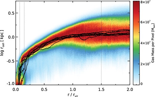
The mass-weighted distribution of gas spatial resolution as a function of radius, for all eight haloes stacked together at L11 resolution. As a proxy for spatial resolution, we show the gas cell sphere-equivalent radii rcell. The dark vertical lines indicate 1.5, 0.15, and 0.07 rvir, the last two bounding the radial range where a density bimodality arises due to the central galaxy. Substructures are excised.
Beyond r/rvir > 1.25 the hydrodynamic resolution is nearly constant, but with a broad distribution spanning from ∼500 pc to ∼3 kpc (physical), depending on what level of overdensity the gas cell resides in. In the halo region, 0.25 < r/rvir < 1.0 the mean resolution scales from ∼400 pc up to ∼1 kpc. The inner halo, typically bounded by r ≲ 0.15 rvir sees the mean cell size decrease rapidly under ∼100 pc as dense gas features associated with the central galaxy begin to dominate. We return to the implications of the relatively coarse halo resolution in the discussion.
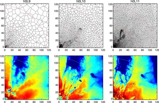
Slice through the Voronoi mesh showing the underlying spatial discretization (top) and a projection through the linearly reconstructed, mass-weighted gas temperature field (bottom) with ∼104 K as blue and ∼106 K as red. The colour mapping to temperature is identical to Fig. 3. The numeric values of the axes labels are in physical kiloparsecs. Halo h0 is shown at z = 2. We include only the upper right quadrant, after centring the halo at the origin, in orthographic projection. The circles denote {0.15,0.5,1.0} rvir, and the projection depth is 238 kpc. The average gas cell size near the virial radius drops with increasing spatial resolution (from left to right), from ∼2.7 to ∼0.8 kpc physical. Note that the exact state of gas in the halo, and the location of satellites, differs somewhat due to timing offsets between the three runs.
Across the bottom row we show a projection of mass-weighted gas temperature, where the colourmap extends from cold, ∼104 K gas as blue to hot, ∼106 K gas as red. Some interesting differences emerge as the gas resolution in the halo increases. The large cold inflow which begins to experience substantial heating at (0.4–0.5) × rvir shows some temperature inhomogeneities at L9, but is essentially a single coherent structure. At L10, this inflow is resolved into a number of smaller gas filaments by the time it crosses half the virial radius. At L11 the temperature structure becomes even more complex, throughout the halo, with small-scale features emerging below the cell-size of the lower resolution runs. Clearly the morphology of accreting gas and its interaction with the quasi-static hot halo material depends on numerical resolution to some degree. In the following sections, we further investigate this dependence by analysing the structure of halo gas at our highest available resolution.
3.1 Visual inspection
We present a visual overview of the eight simulated haloes at z = 2, focusing on the virial scale of haloes 0–3 in Fig. 3, and of haloes 4–7 in Fig. 4, one halo per row. In each case, we show mass-weighted projections of gas density, temperature, entropy, and radial velocity in each column (left to right). All gas cells within a cube of side-length 3 rvir are included, while the temperature of star-forming gas on the eEOS is set to a constant value of 3000 K. The three concentric circles denote {0.15, 0.5, 1.0} × rvir.
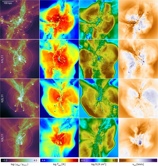
Mass-weighted projections of gas density, temperature, entropy, and radial velocity for the first four simulated haloes at z = 2. In each case, all gas cells within a cube of side-length 3 rvir are included, and distributed using the standard cubic spline kernel with h = 2.5 rcell in orthographic projection. The white circles denote {0.15,0.5,1.0} rvir. Gas density is normalized to the critical baryon density at z = 2. The temperature of star-forming gas on the eEOS is set to a constant value of 3000 K.
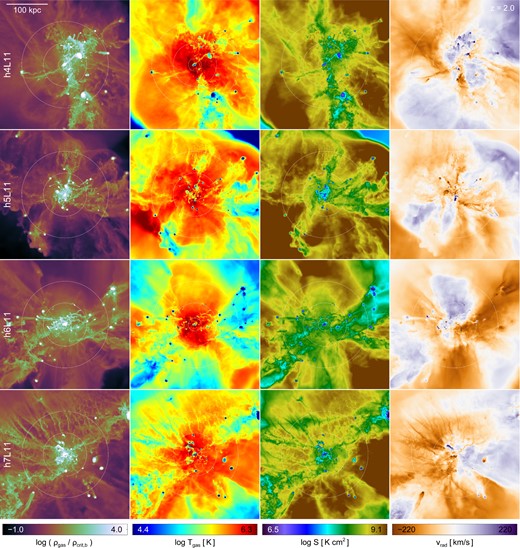
As in the previous figure, mass-weighted projections of gas density, temperature, entropy, and radial velocity at z = 2, but for the other four simulated haloes.
We have separated the eight systems into two groups based roughly on the morphology of their halo gas – the first four haloes (h0–3) are closer to equilibrium at z = 2 and the structure of their hot gas is roughly spherical, whereas the second four (h4–7) are significantly more disturbed. In the first case, the virial shock can be clearly seen as a sharp increase to higher temperature and entropy, typically at ≳ 1.25 rvir. However, the radius of the shock (see also Schaal & Springel 2015) or its existence at all depends strongly on direction, which we explore further in Section 5. These boundaries are also associated with a decreased inflow velocity – that is, radial stalling – as well as increased gas density.
At z = 2 haloes at this mass scale of ≃1012 M⊙ typically reside at the intersection of multiple large-scale filaments (and/or sheets) of the cosmic web. This naturally leads to a significant amount of filamentary inflow across the virial radius. We see that these inflows cover only a fraction of the virial sphere. They can maintain coherency to at least half the virial radius while maintaining a strong overdensity with respect to the mean gas density at each radius. They experience significant heating, typically at ∼0.5 rvir, from ≲ 104.5 K to ≳ 106 K, reaching the peak temperature of the mean Tgas(r) in the inner halo. Their entropy can remain lower than that of the hot halo gas at these radii, ∼108.0−8.5 K cm2 compared to ∼109 K cm2. Although the mass-weighted mean radial velocity inside the halo is generally near equilibrium/zero (denoted by white in the colourmap), we see that in a given direction this is rarely the case, finding instead either non-negligible inflow or outflow velocities.
Finally, we note the existence of interesting features in two haloes, h3 and h7, which have a large number of small, prominent, inflowing streams in the radial range 0.5 rvir ≲ r ≲ 1.25 rvir (see density maps). A detailed analysis of their origin and properties is outside the scope of the current work, and we give here only a heuristic discussion to motivate future investigation. These small streams originate from the lower left direction in the case of h3, and from the top for h7. These filaments are not clearly associated with large-scale structure, and appear to have characteristics distinct from the much larger filaments which are clearly connected to features at larger radii. In particular, although the small streams obtain similarly high inflow velocity, their entropy and temperature are above that of the IGM, and their overdensity with respect to the radial mean is not as significant. Some of the other six haloes exhibit similar features at various points in the past, but they have generally disappeared by z = 2. Qualitatively, we observe that these features can form between one and two times the virial radius semispontaneously, as in an instability, perhaps triggered by perturbations either from substructure debris or the intersection of sheet-like structure in the cosmic web. They are marginally evident at L10 and absent at L9. We reserve an in-depth analysis of the formation of these features and whether or not their growth corresponds to a physical instability in the gas for future work.
We visualize two additional scales, the inner halo structure as well as the large-scale context, of the eight simulated haloes at z = 2. Fig. 5 includes haloes 0–3 while Fig. 6 includes haloes 4–7. The left two columns show the projected density of the gas and stellar components, the white circles indicating 0.05 and 0.15 rvir. The right two columns show the projected density of the gas and dark matter components, the white circles here indicating 1.0 and 2.0 rvir.
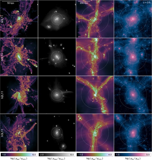
Mass-weighted projections of gas and stellar density at small scales (left two columns), and projected gas density and dark matter density at large scales (right two columns). The first four simulated haloes are shown at z = 2. All gas cells or particles within a cube of side-length 1.0 rvir (small scales) or 5.5 rvir (large scales) are included, and distributed using the standard cubic spline kernel with h = 2.5 rcell (gas) or h = r32,ngb (the radius of the sphere containing the 32 nearest neighbours of the same particle type, for stars and dm) in orthographic projection. The white circles denote {0.05,0.15} rvir (left two columns) and {1,2} rvir (right two columns). Densities are normalized to the critical (baryon) density at z = 2.

As in the previous figure, projections of gas and stellar density on small scales (left two columns), and gas density and dark matter density on large scales (right two columns) at z = 2, but for the other four simulated haloes.
In the centre of the halo, r/rvir ≲ 0.3, the gas component forms a complex morphology with multiple orbiting substructures, commonly associated with tails and gas streams from ram-pressure stripping, as well as tidally induced bridges and spiral patterns. Rapidly varying velocity fields modulate inflowing as well as outflowing material. At r/rvir ≲ 0.05 a large gas disc is a common feature – the final stage in the transformation from large-scale structure and the associated tidal torques to the formation of a galaxy. Here the coherent angular momentum of the halo as a whole must transition to the angular momentum of the forming disc through the complicated dynamics of this inner halo ‘messy’ region (Danovich et al. 2015). In the small-scale views of h2 we see tidal features in the collisionless stellar distribution (extending to the right from the centre), without any corresponding structure in the gas. In h3, we see a massive tidal tail in gas extending out to ≃0.5 rvir (towards upper right of panel), with no corresponding structure in the stars. A recent post-pericentre passage of an ongoing major merger in h4 has induced tidal features in the large companion (upper right of figure) which is still on an outgoing orbit, and generated a long tidal tail, of which the inner half has reversed direction and is falling back on to the central galaxy. A recent merger in h5 has left a double nucleus in the stars, separating by roughly one kpc. In h7 we see a strong tidal warp in the gas and stars of the merging companion (to the upper left of the central), with several stellar shells from earlier minor mergers superimposed. At least some fraction of the narrow inflowing streams in the inner halo are tidal in nature, which highlights the importance of characterizing the origin of gas accretion features – this component of the accretion rate would have been characterized as a ‘stripped’ component in the methodology of Nelson et al. (2015).
In the inner regions of the haloes which we have identified as in equilibrium, the perturbations and gas structures generated by the dynamics of satellite galaxies (see Zavala et al. 2012) are superimposed on a gas background which is aligned at Mpc scales with large-scale gas features. For example, the broad inflow in h0 (towards the top of the image panel) with a width of ∼50 kpc at 0.5 rvir is clearly associated with a gas overdensity extending out to at least 3 rvir. Likewise for the broad inflow in h2 (also, top of the image panel) which has coalesced at the intersection of two such cosmic web filaments. These inflows are not smooth features of constant density gas. They have a ‘wavy’ or rippled appearance, arising from gas density contrasts as high as a factor of ∼103. By visual inspection it is clear that, at least at sufficient resolution, such inflowing filaments are in fact associations of multiple smaller structures with coherent kinematics and origin.
The second set of haloes (h4–7), which are in general more morphologically disturbed, do not show this clear association between small-scale and large-scale gas features. Their time evolution indicates that this is often a consequence of a major halo–halo merger where the two gas reservoirs collide and disrupt any radially coherent gas kinematics as the hot halo re-equilibrates. However, recent major mergers are not always seen, and the nearby environment and topology of large-scale structure also appear to play a significant role in the sphericity of halo gas, independent of assembly history. For example, we consider the number of major mergers with mass ratio η ≥ 1/3 experienced by each halo while the stellar mass is greater than 1010.5 M⊙ (roughly 2 < z < 4), as well as the maximum merger ratio of any merger, under the same constraint. In both cases, the mass ratio is determined at the time the less massive progenitor reaches its maximum stellar mass (see Rodriguez-Gomez et al. 2015). We find that h0, h2, and h3 have had no major mergers exceeding this mass ratio, and indeed none with η ≥ 0.2. The outlier is h1, which did have one major merger (η = 0.8). In the disturbed group, h4 has had four major mergers (with a maximum mass ratio of η = 0.6), h6 has had one (η = 0.65), and h7 has had three (η = 0.95). The outlier is h5, which has had no major mergers satisfying this criterion, the largest mass ratio being η = 0.2.
4 THE PHYSICAL STATE OF HALO GAS
In this section, we quantify the gas behaviours noted above, first by giving the spherically averaged profiles of gas density, cell size, temperature, entropy, radial velocity, and specific angular momentum, and then by examining the pairwise correlation matrix of these same gas quantities.
4.1 Characteristic halo properties
4.2 Radial gas profiles
In Fig. 7 we show the median radial profiles of six gas quantities: temperature, density, radial velocity, cell size, entropy, and specific angular momentum. The main panel plots the profile for each of the eight haloes individually (different line colours) at the L11 resolution level. Light colours are used to indicate the four ‘equilibrium’ haloes, while darker colours indicate the four more ‘disturbed’ systems. The subpanels show the ratio of the radial profiles comparing the L9/L11 and L10/L11 runs, where the thick black lines indicate the average across haloes. We have excised all gravitationally bound substructures, by which we mean satellite galaxies as identified by the subfind algorithm, before constructing mean radial profiles, which would otherwise appear as a forest of small, dense, cold systems in these figures. A few observationally and theoretically motivated scalings with radius are included for reference (dotted and dashed lines).
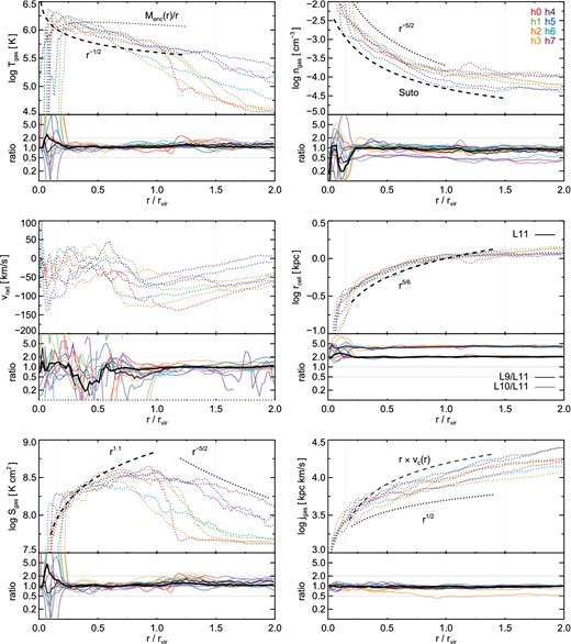
The median radial profiles of six quantities: gas temperature, density, radial velocity, cell size, entropy, and angular momentum. Each halo is shown separately (by colour). The main panels for each quantity show the highest resolution only, while the subpanels show the ratio of the two lower resolution runs to L11 (the mean ratios across all eight haloes are indicated with thick black lines). Various scalings with radius are provided for reference (dotted and dashed lines). All gas within 2 rvir is included, except that substructures are excised.
For instance, going beyond an isothermal model for gas temperature, we can take a gas component tracing dark matter distributed according to an NFW profile. This leads to a scaling of Tgas ∝ Menc(r)/r (e.g. Makino, Sasaki & Suto 1998), which is still much too shallow (dotted line). Instead for r/rvir ≳ 0.15 we have approximately Tgas ∝ r−1/2. Of all eight systems, h0 exhibits the sharpest temperature drop defining an outer boundary of the halo at r ≃ 1.2 rvir, while in most cases there is no sharp transition at or near the virial radius. In all cases the temperature drops precipitously in the inner halo, at 5–10 per cent of rvir. Note that we have assigned a gas temperature of 3000 K to gas on the star-forming equation of state, which would otherwise have an artificially high effective temperature. The Tgas(r) profiles are generally well converged with resolution at r > 0.15 rvir. The mean across all eight haloes and averaged over 0.15 < r/rvir < 1.5 is ≃1.15 for L9/L11 and ≃1.08 for L10/L11. However, physics will dominate resolution – different models for galactic-scale stellar winds or AGN feedback can substantially modify the mean gas temperature profile inside as well as outside rvir (Suresh et al. 2015b).
A gas density scaling as ngas ∝ r−5/2 approximates the mean behaviour of the haloes well, as does a model for an isothermal gas in hydrostatic equilibrium (Suto, Sasaki & Makino 1998, using B = (n + 1)Bp with n = 7, Bp = 1). However, the other panels make it clear that the gas is not in hydrostatic equilibrium, nor isothermal, implying this agreement may be coincidental. Convergence at lower resolutions is reasonable – over the same radial range we find L9/L11 ≃ 0.8 and L10/L11 ≃ 0.9, indicating that the mean gas densities are lower in the lower resolution runs. This is potentially a consequence of better resolving satellite galaxies and their interactions with the central host, which fills the halo volume with more high density gas cells. These are no longer instantaneously bound to the satellite, and so are not excluded – the filamentary feature in the upper-right panel of Fig. 2, extending from ≃0.15 to ≃0.5 rvir is an example of such a tidal tail. The total halo gas mass actually decreases somewhat at higher resolution (∼10 or ∼5 per cent lower for L11 as compared to L9 or L10, respectively), which would otherwise modify gas densities in the opposite direction. Finally, the variable assembly histories lead to the large halo-to-halo scatter, while the sensitivity of merger states to temporal offsets driven by short dynamical time-scales leads to large scatter between resolution levels. As with temperature, however, the caveat is that radial density profiles will depend in detail on the implemented feedback models (Hummels et al. 2013).
We see a similar scatter in the Hubble-corrected gas radial velocities. The haloes have different velocity structures, which commonly feature a slowly increasing inflow velocity down to ∼0.75 rvir, at which point there is a noticeable bump towards an equilibrium value of vrad ≃ 0 km s−1. Until reaching the central galaxy, the radial velocity profiles are then roughly flat. In the following discussion of Fig. 8, however, we show that the mean (or median) velocity profile is an exceedingly poor representation of the dynamics of halo gas. For example, in the mean the quasi-static halo rarely has vrad > 0 for 0.15 < r/rvir < 1.0, while in actuality this value is driven down by the superposition of rapidly inflowing and gently outflowing components.
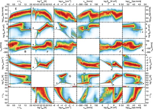
The mass-weighted, two-dimensional correlation matrix between all pairwise combinations of six quantities: gas radius, temperature, density, radial velocity, entropy, and angular momentum. All eight haloes are included and stacked. Each x-axis bin normalized independently, such that the colour mapping reaches its maximum intensity at each x-value, independent of the radial distribution of gas mass. Therefore, panels symmetrically across the diagonal from one another are not simply transpositions, but include additional information. Substructures are excised.
The gas spatial resolution, for which we again use the sphere-equivalent radii rcell as a proxy, becomes better with decreasing radius as expected. Given our constant cell mass refinement criterion, it scales roughly as the cube-root of the density scaling. That is, |$r_{\rm cell} \propto V_{\rm cell}^{1/3} = (m_{\rm cell}/\rho _{\rm cell})^{1/3} \propto \rho _{\rm cell}^{-1/3}$|. At L9 and L10 the cell sizes are a factor of 4 and 2 larger, respectively, scaling with the mean intercell spacing as |$r_{\rm cell} \propto L_{\rm box} N_{\rm cell,tot}^{-1/3}$|.
We overplot the gas entropy profiles with the near-linear scaling Sgas ∝ r1.1 often seen in X-ray observations of local clusters (e.g. George et al. 2009). Despite looking at the significantly more massive cluster PKS 0745−191, ∼1014 M⊙ in the nearby universe (z ≃ 0.1), the inferred radial characteristics from George et al. (2009) are in reasonable agreement with the haloes simulated in this work. A similar level of qualitative agreement is evident at z = 2 for ∼1012 M⊙ haloes in gas temperature, entropy, and density with previous cosmological simulations at L8-equivalent resolution and incorporating more realistic feedback physics (van de Voort & Schaye 2012). In both cases, entropy rises to near the virial radius at which point it flattens and becomes roughly constant. While some haloes exhibit this gradual plateau (h4), the radial entropy profile of others drops as r−2 or faster (h2) at some radius ≥rvir. There is a correspondence between the equilibrium state of the halo and its properties beyond the virial radius – the more disturbed systems (h4–7, darker line colours) generally have higher entropy, without any strong transition. The entropy profiles, averaged over all eight haloes, are well converged with respect to L9 and L10. In the inner halo, h1 and h2 have sharp drops in both Tgas and Sgas at a larger radius than typical, ∼0.25 rvir. In these two cases, while the profiles are properly centred on the galaxy, the galaxy is not entirely centred within the halo. This leads to more cold, low entropy gas beyond the typical disc size.
The specific angular momentum scales roughly as r1/2 or even more accurately as jgas ∝ r vc(r) given the circular velocity vc(r) ∝ (Menc(r)/r)1/2 for an NFW profile of this halo mass. There is broad uniformity among the eight haloes and good convergence in the lower resolution runs, with a small systematic bias towards lower angular momentum content in the halo, L9/L11 ≃ 0.88 and L10/L11 ≃ 0.96, again driven by high-velocity tidal debris becoming better resolved at the highest resolution. In general, for all six properties of the gas explored here, we find reasonable agreement in the radial profiles between the three resolution levels outside of r/rvir > 0.25, with a few notable outliers.
4.3 Distributions beyond radial dependence
To avoid missing important features by averaging over multiple gas populations with distinct properties residing at similar radii, we examine the two-dimensional distributions of these same gas quantities. Instead of only considering their radial dependence, in Fig. 8 we show a full pairwise correlation matrix, every quantity plotted with respect to every other. Here we have stacked together all eight haloes at L11, normalizing only the radius of each gas cell with respect to rvir of its parent halo. Despite the different thermal and dynamical structures of the haloes we verify that the key features seen individually in each are preserved in this collective view. To explore the various relations, we have separately normalized each panel ‘column by column’. That is, for each value along the x-axis, the colour mapping of the corresponding one-dimensional, vertical slice is independent, such that each slice extends from low values (white/blue) through intermediate values (green/yellow) to high values (orange/red). Therefore, there is no global indication of the distribution of mass within each panel (although very noisy regions indicate a poor sampling and therefore comparably little gas mass). In addition, the corresponding panels across the diagonal are not just transpositions of one another, but answer different questions. For example, the Tgas(r) panel in the first column indicates, for each radius, the dominant temperature(s) of gas at that radius, whereas the r(Tgas) panel in the second column indicates, for each temperature, the dominant radius (or radii) of gas with that temperature. We describe some of the more interesting features seen in this matrix, which have been labelled with letters (A)–(M).
Asterisk ‘*’ denotes features which arise in the IGM and disappear if gas at r > rvir is excluded. In particular, all the strong constant entropy features at Sgas ≃ 107.7 K cm2 in the second row from the top, and the near-discontinuities at this same value in the second column from the right.
Regions demarcated with dotted rectangles indicate features arising in the galactic disc or its vicinity, and disappear if gas at r < 0.2 rvir is excluded. This includes all low j gas at high density, which is already above the threshold for star formation in the galaxy. It also includes low-temperature gas which has a radial velocity near zero, as well as the thin horizontal feature of vrad spanning ∼0 ± 100 km s−1 near r = 0 corresponding to a rotating disc. Interestingly, the prominent temperature bridge between the hot halo and galaxy at intermediate densities also largely disappears, indicating that a majority of this cooling occurs at r < 0.2 rvir (see also G).
‘A’ – The virial shock seen as a sharp temperature jump from TIGM ∼ 104.5 to ∼106 K. The width of this transition varies greatly between the eight haloes, h0 being the narrowest at Δr/rvir ≃ 0.1, and as seen here in the stack broadened to Δr/rvir ≃ 0.5 or more. The radius where this transition occurs is typically between 1.25 and 1.5 rvir. After shocking, the temperature slowly increases with radius, following the mean radial profile of the halo, until it reaches ∼0.25 rvir where higher densities lead to accelerated radiative cooling, allowing gas to join the cold ISM phase.
‘B’ – The radial velocity profile of inflowing gas. This component speeds up as it flows in from large distances down to ∼0.5 rvir at which point it largely disappears. The mean velocity is approximately −75 km s−1 at 2 rvir, −150 km s−1 at rvir, and −225 km s−1 at rvir/2. For free-fall from rest at infinity to a point mass of 1012 M⊙ we would expect a speed of −200 km s−1 at twice the virial radius. The actual value is less due the combination of the Hubble expansion and gas dynamics. Given this offset at the halo outskirts, the subsequent scaling is roughly consistent with vrad ∝ r−1/2 as expected from free-fall (i.e. v = (2 GM/r)1/2), at least down to ∼0.5 rvir, below which inflow no longer dominates by mass.
‘C’ – The radial velocity distribution of the hot halo gas. These two components overlap between 0.5 < r/rvir < 1.0 as gas transitions from rapidly inflowing to quasi-static. This ‘equilibrium’ component is not truly at rest, however, since a large mass of gas has positive radial velocity. Gas with vrad > 0 arises from the dynamical formation of the halo atmosphere and associated splashback motion in the baryons (e.g. Wetzel & Nagai 2015). In this stacked view the radius of this transition is notably interior to the virial shock, ∼0.75 rvir as compared to ∼1.25 rvir. Investigating the haloes individually, we conclude that this radial offset is largely a misleading feature arising from the stacking of radially averaged velocity profiles. Instead, the radius of a strong jump in temperature and entropy also closely corresponds to a sudden decrease of inward velocity, as a result of the transfer of kinetic to thermal energy.
‘D’ – The virial shock seen in a sharp entropy jump from the nearly constant value in the IGM of ∼107.7 to ∼109 K cm2 characteristic of the maximum obtained in the hot gas for haloes of 1012 M⊙ . The entropy increase occurs over a narrower radial range than the corresponding temperature increase, and at a slightly smaller radius with respect rvir. This may be indicative of pre-shock compressive heating, although we caution that this radial difference varies from halo to halo and as shown in the stack. For example, in our subsequent exploration of h0 in Fig. 11 we see that there is a close correspondence between the radii of temperature and entropy jumps. After shocking, the entropy slowly declines with radius, following the mean radial profile of the halo.
‘E’ – The angular momentum distribution is unimodal and scatters about its mean profile, with no evidence for multiple populations of gas having distinct jgas at any radius. Interestingly, this is the only property from Fig. 7 which is well converged at r/rvir < 0.25, and together with gas density is one of the few for which the full distribution as a function of radius is well characterized by its mean profile.
‘F’ – The radial velocity depends somewhat on the temperature of the gas, with the hottest gas populating the high positive velocity tail, while cold gas is inflowing. At all temperatures there is a continuous distribution of radial velocities, with an upturn at ∼106 K, above which gas has a mean radial velocity consistent with zero, and below which the mean vrad is always negative (see also Joung et al. 2012). The rapidly inflowing hot gas, discussed in (C), is the high velocity tail of the gas distribution at these temperatures and so subdominant by mass.
‘G’ – The usual ‘phase-diagram’ plotted for cosmological simulations. Cold, low density gas (ngas ≲ 10− 4 cm−3) in the IGM (denoted by a star) occupies the lower left corner, the tight relation with T ∝ n2/3 indicative of adiabatic compression. Shock-heated gas at intermediate densities is the only source for T > 105.5 K gas. At higher densities (ngas ≳ 10− 3 cm−3) strong cooling flows develop at small radii, after which gas approaches the effective temperature floor of ∼104 K until it reaches the star formation threshold at nH = 0.13 cm−3.
‘H’ – The heating of inflow, seen here as the dominant temperature for gas at each radial velocity. The handful of strong vertical features are largely an artefact of the stacking. In Fig. 9 we show a single row of the correlation matrix, restricted to only gas with 0.2 < r/rvir < 1.0 and so definitely in the halo, as opposed to the galaxy or the IGM. With this restriction we find a clear correlation between deceleration and heating, with the colder component at higher inward radial velocity. Cold gas below ≃105.75 K is rapidly inflowing with large negative vrad, and transitions above this temperature to a mean inflow velocity consistent with zero. This occurs decidedly interior to the virial shock, and outside the galaxy.
‘J’ – The average radial velocity as a function of entropy, restricted to gas in 0.2 < r/rvir < 1.0 (as shown in Fig. 9) resolves nicely into two distinct populations, where material with Sgas ≳ 108.5 K cm2 has a mean vrad = 0 which is roughly constant. On the other hand, gas with lower entropy than this threshold has a mean vrad ≃ −150 km s−1, with a gradual trend towards faster inflow with lower entropy.
‘K’ – Similarly, the average radial velocity as a function of angular momentum, restricted to gas in 0.2 < r/rvir < 1.0 resolves nicely into two components. Gas with j ≲ 104.25 kpc km s−1 has zero mean radial velocity, whereas higher angular momentum gas has vrad ≃ −vvir (see Fig. 9). The two populations overlap for 104.25 < jgas < 104.5. Together with (J) this panel shows the distinct physical properties of the quasi-static and inflowing halo gas.
‘L’ – Star-forming gas has a temperature on the eEOS, which is set to a low, constant value to differentiate it from other gas. This results in the constant temperature band at ≃103.5 K across this entire row. This gas is restricted to small radii, high densities, low radial velocities, and low angular momenta.
‘M’ – Gas with high entropy, S ≳ 108 K cm2 has a well-defined relation to radius, following the mean halo profile. Below this threshold, if we exclude material in the IGM, gas at any given entropy is essentially distributed throughout the entire halo.
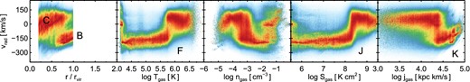
Two-dimensional distributions of gas mass in the planes of radial velocity versus radius, temperature, density, entropy, and angular momentum. As in the vrad row of Fig. 8, except that here we add the requirement that gas cells reside within 0.2 < r/rvir < 1.0 in order to include only halo gas, removing both the central galaxy and the IGM. Two broadly distinct gas components are clearly present: the colder component has higher density, lower entropy, higher angular momentum, and dominates at large radii, while the hotter component has lower density, higher entropy, lower angular momentum, and is dominant within ∼0.6 rvir.
We have seen in several cases how the mean or median radial profiles fail to fully capture the full state and structure of halo gas. Clear examples are the distributions of temperature, entropy, and radial velocity as a function of radius. On the other hand, the distributions of density and angular momentum as a function of radius are comparatively well described by a median and scatter. By measuring average properties within radial bins we implicitly assume that the structure of halo gas is spherically symmetric. Even Fig. 8 fails in this regard. For instance, the finite radial thickness of the temperature jump associated with the virial shock could either arise from (i) a spherically symmetric feature of that same thickness, or (ii) the superposition of many thin shocks spread throughout the same radial range, different shock fronts existing at different radii depending on direction. Motivated by the latter possibility, we proceed to investigate and quantify any variation of the structure of halo gas as a function of angle on the sphere.
5 ANGULAR VARIABILITY
As a first step away from radial averages, we consider the properties of gas in a broad radial shell encompassing the regime of interaction between quasi-static material and filamentary inflow. In Fig. 10 we plot the distributions of temperature, density, radial velocity, and entropy, for all gas cells within 0.5 rvir < rgas < 1.0 rvir. In particular, we examine how well the lower resolution runs reproduce the distributions of these quantities found in the highest resolution (L11) runs. In this radial range, we find that the gas of all simulated haloes has broadly similar properties, differing only in the details.
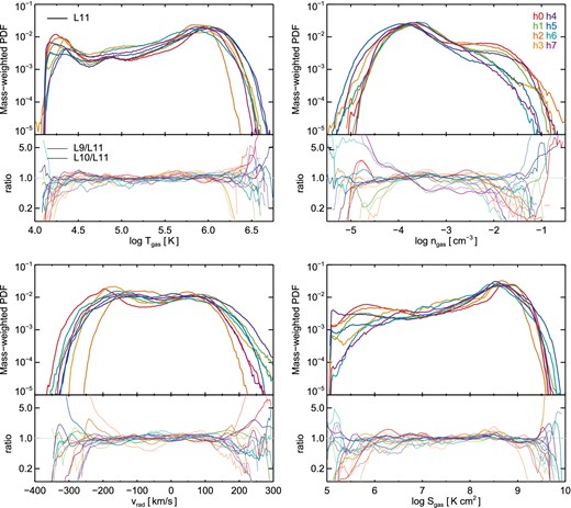
The mass-weighted PDF of instantaneous gas temperature, density, radial velocity, and entropy, restricted to the radial range 0.5 rvir < rgas < 1.0 rvir. The upper panel shows all eight haloes at the highest resolution level (L11, different colours), while the subpanels below show the ratio of the two lowest resolution levels to the highest, L9/L11 (thin lines) and L10/L11 (medium lines). The vertical axes of the ratio subpanels are logarithmic from 0.1 to 10. For the most part, the eight haloes show similar structure and their lower resolution counterparts scatter about the L11 distributions (see text for details).
The temperature distribution (upper left) shows a broad peak centred roughly at Tvir, slowly falling off towards lower temperatures and with a distinct low temperature peak at ≃104.25 K. While the fractional amount of gas at each temperature in the L9 and L10 runs can differ throughout this regime by up to a factor of 2, depending on halo, the mean ratio of both L9/L11 and L10/L11 is consistent with unity from 104.5 to 106.0 K. At the highest temperatures >106.25 K the lower resolution runs have much larger deviations with respect to L11, but we attribute this primarily to poor sampling of the extreme tail of the distribution due only to a low number of available gas cells. In contrast, the PDF at the low temperature peak is systematically lower in the lower resolution runs. At ≃104.25 K where there are still a large number of gas cells, the mean across all eight haloes is L9/L11 ≃ 0.5 and L10/L11 ≃ 0.8, indicating that there is a smaller fraction of the total gas mass at these temperatures at lower numerical resolution. Note that 104 K is effectively the temperature floor due to cooling in these simulations, and the mean TIGM at redshift two is just above this value. We caution that the amount of gas at these intermediate temperatures will increase due to modifications to the net cooling curve when metal line cooling is introduced, and this effect is neglected in the current simulations.
Gas density shows an even larger variation on a halo to halo basis – some have a strong second peak at higher densities, while this feature is largely absent for the less relaxed haloes. The ratio with respect to the lower resolution runs is largely consistent with unity for −4.0 < log (ngas[ cm−3]) < −2.5. Between the upper value and the star formation threshold of ≃10−1.0 cm−3, there is a decrease, at lower resolutions, in the fractional amount of gas at such densities. In this range, the mean ratio across all eight haloes is L9/L11 ≃ 0.4 and L10/L11 ≃ 0.6. As with temperature, we see that the density PDFs can disagree between resolutions by as much as a factor of 10, but only in the tails when the magnitude drops to low values of ≤10−4. The disagreement is similar with radial velocity, where the mean Ln/L11 ratios are consistent with unity for all values away from the extremes.
The distribution of vrad itself is comprised of two broad components, which depending on halo can be centred anywhere between 0 and −100 km s−1. The positive and negative peaks are indicative of outflow and inflow, respectively. The primary driver of interhalo variation – for example, that h0 has smaller minimum and maximum velocities – appears to be differences in assembly history, particularly a recent merger with another massive halo, or lack thereof. We explore this further in the following section. Finally, gas entropy behaves similarly to temperature, where we find that low entropy gas is strongly subdominant by mass with respect to the high entropy hot halo material. The largest variation between haloes occurs for log Sgas < 106 K cm2, down to the floor at ≃105 K cm2. The halo-average PDF at L9 and L10 reveals a smaller fraction of gas at these lowest entropies when compared to the L11 run.
In general, we conclude that for any given halo, large variations between the three resolution levels can be seen, with deviations up to a factor of 10 in the fractional amount of gas at a particular temperature, density, radial velocity, or entropy. These deviations occur mostly in the tails of the distributions which are poorly sampled at the lower resolution levels. Furthermore, the timing differences present in any single comparison likely influence some of the largest outliers. With respect to the average behaviour across all eight haloes, we find that the lower resolution runs have less low temperature, high density, and low entropy gas. By mass fraction with respect to the total gas mass in this radial range, the magnitude of the effect is ∼2 (∼1.5) in L9 (L10), for all three of these gas properties.
5.1 Structure along radial sightlines
To proceed, we consider sightlines originating outwards from the halo centre in different directions, which will have different radial structure. If the hot halo gas was triaxial, for example, we could anticipate that the radius of a strong virial shock would differ along its major and minor axes. We therefore measure the angular variability of the thermal and dynamical structure of the halo by casting many such sightlines from the centre of each halo. Along each of these ‘radial rays’ we sample the continuous fields of gas temperature, radial velocity, entropy, density, and angular momentum in fixed steps of Δr. Using this ensemble of rays we can then quantify the structure of halo gas without binning in spherically symmetric radial shells.
Ray directions are set using the healpix discretization of the sphere (Górski et al. 2005) into equal area pixels, which implies equal angular spacing of rays at all refinement levels. The total number of radial rays is |$N_{\rm ray} = 12\,N_{\rm side}^2$|, corresponding to an area subtended by each ray equal to |$\Omega _{\rm ray} = 4 \pi / 12\,N_{\rm side}^2$| sr, or |$\theta _{\rm ray} = (180^2 / 3 \pi N_{\rm side}^2)^{1/2}$| deg. The sampling in the radial direction is linear and controlled by the parameter Nrad such that Δr/rvir = 2.0/Nrad. Our fiducial parameters of Nrad = 400, Nside = 64 result in a sampling of Δr ≃ 0.5 kpc and Δθ = 1 deg. At each point, mean gas properties are estimated with a tophat kernel with adaptive size equal to the radius of the sphere enclosing the Nngb = 20 nearest gas neighbours. This is close to the mean number of natural neighbours (or cell faces) of the evolved Voronoi mesh in a cosmological simulation (Vogelsberger et al. 2012). Therefore the spatial scale of this effective smoothing is approximately matched to the scale of the stencil used in gradient estimation for linear reconstruction of fluid quantities in the MUSCL-Hancock scheme of arepo (Springel 2010).
In Fig. 11, we show a snapshot of the combined radial and angular structure of a single halo (h0L11) at z = 2. The 12 demarcated intervals along the y-axis denote the 12 base pixels of the healpix discretization. Within each base pixel the nested ordering scheme uses a hierarchical quad-tree to preserve adjacency, and the four subintervals delineate the top nodes of each such quad-tree, implying that structure seen in the vertical direction is spatially coherent within these major and minor intervals. We note that there is no mass weighting or, for that matter, any indication of the mass distribution within each of the five panels, since the sampling points are smoothly distributed throughout the volume regardless of the underlying gas cell distribution.
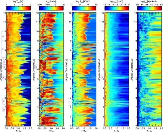
The angular variability of gas temperature, radial velocity, entropy, density, and angular momentum at a given radius. Each pixel along the vertical direction represents a single radial ray, which are equally spaced in angular separation. The radial variability of the virial shock is evident in the shifting boundary between dark blue and yellow/orange in the left-hand panel. Penetration of low-temperature gas to radii smaller than rvir correlates with higher inflow velocities, lower entropy, and higher density, often extending out into the IGM at r ≥ 2 rvir. In this figure we include only a single halo, h0L11, with Nside = 16, Nrad = 100. All substructures other than the primary have been excised, thereby excluding satellites.
Focusing first on the temperature structure we clearly see a boundary separating the cold, IGM from hot, virialized gas. At this halo mass scale, the temperature increases by roughly two orders of magnitude, from ≃104 to ≃106 K (dark blue to yellow/orange). In some directions this heating is coherent and occurs at essentially uniform radius (for example, 9–10, marked ‘A’), demarcating a clear ‘virialization boundary’. However, across all sightlines we also observe a temperature jump of similar magnitude anywhere from 1.0 < r/rvir < 1.5, and smaller jumps can occur out to twice the virial radius. Even so, from Fig. 3 we know that this halo is one of the most spherically symmetric, with a noticeable transition in the state of gas just outside the virial radius. In directions where the gas temperature is warm and exceeds ∼105 K out to twice rvir, we find a correspondence to a baryonic overdensity, with respect to mean at that distance. This is indicative of large-scale gas filaments and the heating associated with their earlier collapse.
Interestingly, in directions where gas coherently penetrates to radii smaller than the virial radius and remains cold (e.g. B), this same correspondence to overdensities at larger distance remains. Qualitatively, the existence of an inflowing gas filament arising from the cosmic web suppresses a strong shock at the virialization boundary. This can arise from previous heating from filament formation outside of the halo, which increases the gas temperature to an intermediate state between TIGM ∼ 104 K and Tvir. There can none the less be a (smaller) temperature jump around the mean virialization boundary (C), although this is not always true and gas can gradually heat seemingly all the way to the peak of the halo temperature profile just exterior to the disc region (e.g. D). Alternatively, this shock suppression can also arise from a delay of strong heating to deeper within the halo, in which case there is less preheating evident at large distances. The radius of the strongest temperature jump then decreases, typically to 0.25 rvir < r < 0.75 rvir as in much of (E). There are essentially no sightlines along which the gas does not experience heating above TIGM at some radius. Since the velocity field, and so the streamlines of accreting gas, are not purely radial, this does not preclude the possibility that gas could avoid heating along its actual dynamical path. Such a trajectory would be curved in these panels. In some cases (F) we can largely rule out this behaviour, since over a large coherent solid angle no cold gas at r < 0.5 rvir is directly connected to cold gas at larger radii. In general, given inflow structure which is coherent in space and coherently evolving, this analysis method can inform on gradients in gas structures even for non-radial flow. In general, however, the analysis based on radial rays is limited in this respect, particularly when such inflows are fragmented and have complex interior structure in any given gas property.
As with density, we also see a strong correlation between temperature and both entropy and radial velocity. Strong temperature jumps just outside the virial radius are also evident as sharp transitions from the gradually increasing (negative) IGM inflow velocity, through equilibrium, to a generally (positive) outflow speed indicative of the virialized halo gas. In some directions (G) multiple components are clearly visible, where an inner halo is comprised of hotter, denser, and more rapidly expanding gas which has more recently bounced back under its own thermal pressure. Similarly, the entropy of the low-density IGM undergoes a sharp increase before declining towards the halo centre. On a sightline by sightline basis the radius of the entropy jump is nearly equal to that of the temperature and radial velocity jumps. Finally, the angular momentum of the gas is clearly the least affected by the virialization boundary. As the velocity field becomes increasingly complex towards smaller radii, the non-radial component contributing to the angular momentum does not have a clear correlation with any of the other local gas properties.
5.2 Different gas heating regimes
To understand the properties and the importance of sightlines exhibiting different radial behaviours, we would like to identify a few characteristic types. We separate rays into a small number of disjoint sets in Fig. 12, each group ideally having a distinct radial behaviour. By visual classification we identify four such groups, which together encompass the majority of sightlines. In particular, we split rays into ‘distant shock’, ‘closer shock’, ‘gradual heating’, and ‘low entropy’ types, each of which is based on a quantitative selection applied across some radial range. Specifically, for the ‘distant shock’ type we require both where dT/dr denotes the derivative of gas temperature with respect to radius, in units of (log K)/(0.1 rvir), rmax(Q) indicates the radius where the quantity Q reaches its maximum value, and |$Q|_{r_1<r<r_2}$| indicates that a quantity Q is constrained only within the radial range between r1 and r2. For the ‘closer shock’ type we require That is, both must exhibit a strong temperature jump at either large or intermediate radii. Of the remaining rays not meeting the prior two conditions, we further require rays of a ‘gradual heating’ type to satisfy Finally, the ‘low entropy’ type requires of any remaining rays In Fig. 12 we show all four groupings as separate panels (for halo h0L9). The temperature is plotted as a function of radius, while colour indicates gas entropy. A single prototypical ray is included as a thick line, while all rays belonging to that type are shown underneath as thin lines. The mean radial velocity profile of all rays of that type, locally averaged in radius, is denoted by the series of numbers shown in each panel, in units of km s−1 (negative denoting inflow). The top inset above each panel plots the temperature derivative dT/dr, positive denoting increasing temperature with decreasing radius, for the prototypical ray (thick) and five other random sightlines of that type (thin).
max(dT/dr|0.2 < r < 2.0) > 0.25,
1.5 < rmax(dT/dr) < 2.0,
max(dT/dr|0.2 < r < 2.0) > 0.25,
0.8 < rmax(dT/dr) < 1.5.
max(dT/dr|0.2 < r < 2.0) < 0.8.
max(Sgas|0.2 < r < 2.0) < 8 × 10⁸ K cm2.
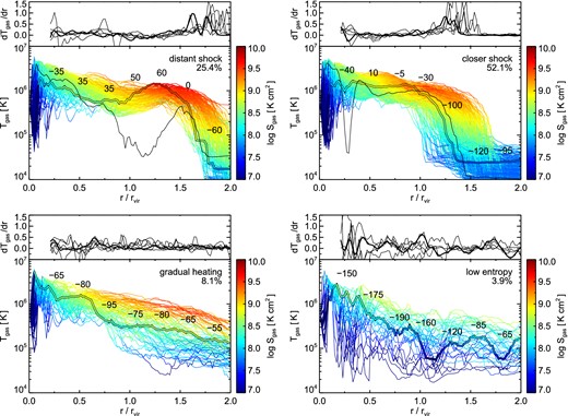
The temperature profiles of individual radial rays (four main panels), with colour indicating gas entropy. For clarity we include only one halo, h0L9, with Nside = 8 and Nrad = 100. Each of the four panels includes a disjoint subset of the entire ray set, where the selection for each was chosen by visual inspection in order to find four types of sightlines, each with similar radial properties, which together cover the majority of behaviours. In each panel, all rays are shown as thin lines, while a single prototypical example is shown as a thick coloured line. The mean radial velocity profile for each ray type is indicated by the series of numbers (in units of km s−1, negative denoting inflow, the standard deviation of which roughly increases from ∼30 km s−1 at large radii to ∼80 km s−1 in the inner halo). The smaller top insets show the derivative of gas temperature with respect to radius, in units of (log K)/(0.1 rvir). The percentage in each panel indicates the fraction of all rays satisfying the criteria, for this particular halo. Given our selections, some sightlines are excluded from all four types. The vast majority of these rays either fall just outside a selection, or experience a significant temperature dip within the halo, which is a signature of satellite debris or intersection with non-radial filamentary inflows. Two such examples are shown as thin black lines in the upper two panels, which are otherwise excluded for visual clarity.
We briefly describe the behaviour of each type. Sightlines experiencing a ‘distant shock’ undergo a jump in temperature from ≃104 to ≃106 K over a radial range of ∼0.1 rvir (although, as in the example, multiple jumps can exist and be spread over a larger radial range). At this same radius the entropy also increases by approximately two orders of magnitude, from ≃107.5 to ≃109.5 K cm2. The rapid inflow velocity decreases, reaching its maximum (positive) value near the radius of maximum temperature. Towards smaller radii, the ray temperature then follows the steadily increasing mean temperature profile of the halo, until reaching the centre. The ‘closer shock’ sightlines have the same behaviour – the radial distinction between close and distant shocks is arbitrary. In either case, the temperature profile can be non-monotonic if the shock occurs at sufficiently large radius, such that the shock temperature is greater than the local mean Tgas(r), and the gas can subsequently cool. Heating can be associated with one or multiple shocks (e.g. two, in the case of the prototypical example shown in the upper-left panel). The maximum derivatives of temperature and entropy are ≃2.0 (in log) per 0.1 rvir, although the typical maximum along any given ray is roughly half as large.
The ‘gradual heating’ sightlines generally reach the same maximum temperature (in the inner halo) and entropy (near the virialization boundary), but do so without any sudden jumps. Here the inflow velocity is roughly constant and always negative, never approaching a quasi-static state, increasing towards smaller radii and with a mean of approximately −75 km s−1. The ‘low entropy’ rays are selected to have a maximum entropy of less than 8 × 10⁸ K cm2, although the exact value is arbitrary. In this case, the inflow velocity is always strongly negative, peaking in the inner halo, with a mean of approximately −135 km s−1. The vast majority of these rays still reach high temperature, but at ≲ 0.25 rvir and possibly not until the disk-halo interface. At r > 0.5 rvir we see that ‘low entropy’ sightlines also have systematically lower temperatures and higher inflow velocities than the other three types.
In Table 3 we include the fraction of each of these four ray types, calculated as the mean over all eight haloes. Although the balance between the two shock types shifts with resolution, the total ray fraction experiencing a strong shock remains at ≃60 per cent, with the temperature jumps moving somewhat inwards. The gradual heating fraction is also relatively constant with resolution at ≃30 per cent, while the low entropy ray fraction drops gradually from ≃4 per cent at L9 to a negligible fraction by L11.
The percentage of radial rays of each of the four types: ‘distant shock’, ‘closer shock’, ‘gradual heating’, and ‘low entropy’. The mean fraction across all eight haloes is calculated separately for each resolution level. Since rays cover equal angular area, each fraction corresponds to the geometrical percentage of the sphere occupied by sightlines satisfying each criterion. The errors represent the standard deviation among the eight haloes.
| Type | L9 | L10 | L11 |
|---|---|---|---|
| Distant shock | 26.4 ± 5.1 | 21.3 ± 5.7 | 22.9 ± 10.7 |
| Closer shock | 29.8 ± 14.0 | 34.8 ± 15.0 | 44.8 ± 17.6 |
| Gradual heating | 27.4 ± 14.8 | 29.1 ± 11.2 | 27.6 ± 11.0 |
| Low entropy | 4.3 ± 1.1 | 2.4 ± 1.2 | 0.3 ± 0.2 |
| Type | L9 | L10 | L11 |
|---|---|---|---|
| Distant shock | 26.4 ± 5.1 | 21.3 ± 5.7 | 22.9 ± 10.7 |
| Closer shock | 29.8 ± 14.0 | 34.8 ± 15.0 | 44.8 ± 17.6 |
| Gradual heating | 27.4 ± 14.8 | 29.1 ± 11.2 | 27.6 ± 11.0 |
| Low entropy | 4.3 ± 1.1 | 2.4 ± 1.2 | 0.3 ± 0.2 |
We have verified that these values, and all the other quantitative results related to the radial rays, are well converged with the numerical parameters Nrad = 400, Nside = 64. Given our selections, approximately ≃10 per cent of the sightlines remain excluded from all four types at L9, this value decreasing to ≃4 per cent at L11. The vast majority of these excluded rays either (i) fall just outside a selection, or (ii) experience a significant temperature dip within the halo. By definition they do not satisfy the ‘gradual heating’ or ‘low entropy’ conditions. Two such examples are shown as thin black lines in the upper two panels. We find that the narrow dips are typically a signature of intersecting satellite debris or satellite outskirts, which were not calculated as locally gravitationally bound and so were not excised. Gas cells of this type fill a larger fraction of the halo volume at higher resolution, leading to the increased percentage of rays excluded from all four types. Broader dips are typically intersections with large filamentary inflows which are not aligned in the radial direction. This exposes the main caveat of the above analysis – namely, that gas inflow with a tangential velocity component need not evolve according to the temperature, entropy, or velocity structure of any particular radial ray.
5.3 Quantifying the asphericity of temperature
In order to quantify the instantaneous halo temperature structure, we calculate differential histograms of radii satisfying a given criterion in Fig. 13 (top panel). Solid lines show the distribution of the maximum radius, for each radial ray, where the temperature exceeds some fraction of Tvir (different colours). To avoid washing out features by stacking, we include only one halo (h0L11). We see that for the three lowest temperature cuts, (0.1–0.5) × Tvir, the rmax values all show a strong peak at ≃1.2 rvir, indicative of the virialization boundary. The distributions are broad, however. In the case of T/Tvir > 0.5 the spread of maximum radii is roughly symmetric, extending from 0.5 rvir out to 1.6 rvir. That is, although the majority of sightlines first exceed 0.5 Tvir at a well-defined surface sitting at 1.2 rvir, a non-negligible fraction first exceed this temperature already by 1.6 rvir, and an even larger fraction cross this threshold inside the virial radius, between 0.5–0.75 rvir.
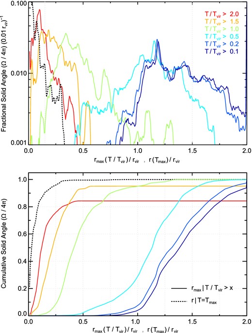
Top: the histogram of radii satisfying two different temperature criteria (different linestyles), computed separately for each radial ray. Since each subtends equal angle, this histogram is equal to the fractional solid angle of the whole sphere covered by rays satisfying each criteria, as a (differential) function of radius. The criteria are: (i) the maximum radius at which the temperature along the ray exceeds some fraction of Tvir, in solid coloured lines, and (ii) the radius at which each ray reaches its maximum temperature, with the dotted black line. For the first condition, we consider six different temperature thresholds (from blue to red). In this figure we include only one halo at the high-resolution level, h0L11, with Nside = 64 and Nrad = 400. Bottom: as in the upper panel, but here as a cumulative function of radius.
The three higher temperature thresholds (green, orange, red) reflect the increasing mean radial temperature profile of the halo. The virial temperature is typically reached at ≃0.5 rvir, while gas reaches twice Tvir just prior to the galaxy at ≃0.1 rvir. We see that the peak of the radial distribution, for rays satisfying rmax(T/Tvir > {0.5, 0.2}), measures the most dominant radius for this transition. With respect to halo to halo variability, we find that the shapes and overall widths of each rmax distribution can vary substantially. For instance, h0 has a strong peak which is both the narrowest in radius and the most covering in angular fraction. Yet, it also has a prominent secondary peak of roughly half the geometrical importance at larger radius, Δr ≃ 0.2 r/rvir further from the halo centre. Even more extreme, h3 has two peaks of equal strength spaced Δr ≃ 0.5 r/rvir apart. Multiple radial peaks are a common occurrence.
The widths of the distributions also encode a measure of the spherical symmetry of any strong heating. Here it is useful to look at the cumulative histograms of radii satisfying these same temperature criteria, as shown in the bottom panel of Fig. 13. The slope of this cumulative histogram indicates angular uniformity – presence of a Heaviside step function would imply perfect spherical symmetry, while slopes approaching zero would mean that the temperature transition takes place, depending on sightline, over widely disparate radii. The fact that several temperature thresholds plateau below unity indicate that only ≃85 per cent of rays reach T > 2.0 Tvir (red line) and ≃95 per cent of rays reach T > 1.5 Tvir (orange line), while all other temperature thresholds are exceeded along all sightlines. Any value for the cumulative solid angle can provide a good way to quantify the location of the mean virialization boundary. For instance, the radius by which 2π sr are covered by rays with maximum temperature exceeding half of Tvir is ≃1.1 rvir. Finally, the dotted black line plots the distribution of the radius where each ray reaches its maximum temperature, which is peaked in the halo centre due to the shape of the halo temperature profile.
We conclude with two visual impressions of the three-dimensional temperature structure in and around a single halo (h0L11). First, it is illustrative to separately show the distributions of hot and cold gas components within the halo to avoid any confusion arising from mass-weighted temperature projections, as used in the second columns of Figs 3 and 4. Every pixel in such a projection will contain a mean temperature along that direction, which could be an intermediate value resulting from the admixture of distinct cold and hot gas components. In exploring the angular variability of halo gas structure in Fig. 11, we have already attempted to avoid this issue and capture the full temperature information without any binning or averaging. However, as gas does not necessarily flow along purely radial trajectories, the evolution in radius which we have emphasized does not necessarily reflect the time evolution of the thermodynamic properties of any given gas parcel. As previously mentioned, a quantitative exploration of the thermal evolution of inflow requires the use of the tracer particle scheme (Genel et al. 2013) and will be the focus of future work. At present, Fig. 14 shows a gas temperature projection including only gas which has instantaneous temperature below (left-hand panel) or above (right-hand panel) 0.1 Tvir (∼105.1 K). We see features which may not have been readily apparent in the previous figures – complex structure remains visible in the colder component to small radii (<0.5 rvir). As this inflow reaches the inner galaxy, streams have fragmented into narrower substreams, as discussed in Section 3. Some of the components of these inflows are cold, roughly 10 times colder than the surrounding hot media, even up to the point where they ‘meet’ the central galaxy. Since hot halo gas must exist along all sightlines within the virial radius, the mass-weighted temperature projection will give the biased impression that cold gas at small radii is warmer than the physical temperature of individual cold gas cells. This important caveat should be considered with this visualization technique. Physically, the increasing density of the inner halo implies correspondingly faster cooling rates, which at some point must enable gas to join the cold star-forming ISM of the disc. The radial distribution of cool gas in the inner halo, how it arises and is maintained at that point, and indeed the radii at which inflow first experiences significant heating, are all questions which remain to be quantitatively explored.
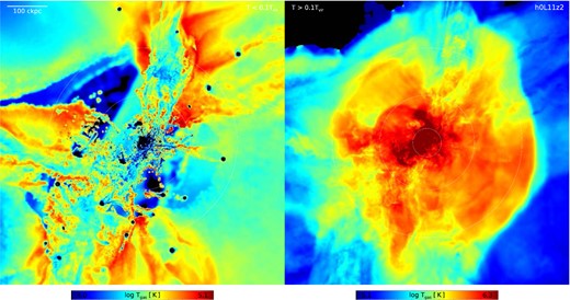
Mass-weighted projections of gas temperature for a single halo, h0, as in the second column of Fig. 3, except that we here separate gas based on its instantaneous temperature to avoid possibly confusing projection effects. The left-hand panel includes only gas with T < 0.1Tvir (∼105.1 K), while the right-hand panel includes only gas with T > 0.1 Tvir. Note that the images have different colour table scalings.
Finally, in Fig. 15 we highlight larger scale structure with a volume rendering of five iso-temperature surfaces using the same blue–red colourtable and physical bounds of 4.4 < log Tgas [K] < 6.3 as in the temperature projections of Fig. 3. It is sampled with a transfer function comprised of four narrow alpha-channel Gaussians at log Tgas [K] = {4.5, 5.0, 5.5, 6.0} with widths of σ = {6, 6, 3, 3} × 10−3 in log K. The scale of the image is 5.5 rvir in both height and depth, as in the zoomed out panels of Fig. 5. The dark blue surface straddles the mean TIGM at ≃2 rvir and reveals a morphology at overdensities just below cosmic web filaments. The light blue surface at 105 K clearly outlines the structure of Mpc-scale, large-scale filaments, while the yellow surface at 105.5 K is restricted to the interior of warmer filaments. Both of these two iso-temperatures surfaces are closed. Further, they enclose the virialized halo itself – we can see how the filamentary shape of the 105 K surface at r > 2 rvir transitions smoothly into a quasi-spherical shape by opening up, wrapping around and encompassing the higher temperature shells. The mean radius of the 105.5 K surface is ≃1.0 rvir, while that of the 106 K surface is ≃0.5 rvir. The intersection of radial sightlines cast outwards in different directions with this complex temperature structure in and around the 1012 M⊙ halo gives rise to the four distinct ray types described earlier.
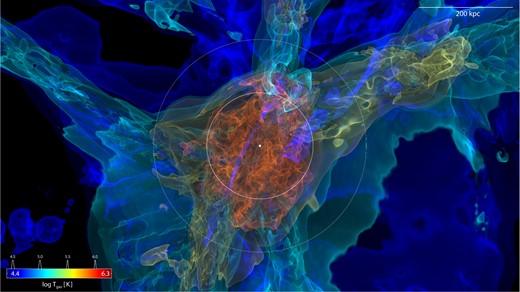
A volume rendering of the three-dimensional temperature structure around a single halo (h0L11) at z = 2. We use an orthographic projection with depth and height equal to 5.5 rvir (≃620 kpc), as in the zoomed out panels of Fig. 5. The colourtable and 4-Gaussian transfer function are shown. A front-to-back ray tracing method is used, with no scattering and no absorption. Along each ray we sample with a constant step-size of 0.25 kpc. The temperature at each sample point is calculated using the standard cubic-spline SPH kernel interpolant with adaptive smoothing length h over the N = 200 nearest neighbours (the representation of the gas in terms of a Voronoi tessellation is not used). We choose this rather large smoothing scale to focus on the large-scale temperature structure of the halo, at the expense of visualizing very small scale features. The white dot marks the halo centre, and the white circles denote one and two times the virial radius.
6 DISCUSSION
The eight haloes simulated in this work were selected randomly from a parent box with a side-length of 20 h−1 Mpc ≃28.6 Mpc – that is, no additional properties of the haloes such as assembly history or environment were explicitly considered. The relatively small periodic box size is a compromise between achieving high resolution while also capturing massive objects as well as large-scale dynamical effects. This decision could have undesirable consequences. For example, the truncation of the power spectrum on scales larger than the fundamental mode allowed by the box can reduce the strength of clustering and suppress the growth of large density peaks. However, we expect this effect to be negligible at the relatively early stopping time of z = 2, and in any case not to qualitatively modify the assembly histories or internal structure of the haloes we consider in this work (Power & Knebe 2006).
Of more concern is a potentially unusual environment. Our parent simulation represents a single realization of the stochastic initial noise field, while the true universe contains numerous such realisations. This cosmic variance means that applying our selection procedure to another randomly chosen parent box could yield eight haloes with different properties. In particular, proximity to a large cluster or a protocluster environment could have a significant impact (e.g. Dressler 1980; Kauffmann et al. 2004). As expected from its small size, there are no massive clusters represented in our parent box. At z = 2 the most massive halo has a total mass of ≃1012.5 M⊙, and only five haloes exist which have masses greater than the upper limit of our mass range selection. This implies that, of the 25 most massive haloes in the parent box, nearly a third were selected for re-simulation, and our eight haloes could be biased simply due to sampling variance arising from a finite box size. By redshift zero, the haloes discussed here have diverse evolutionary paths. The first four, which we observed to be in general more relaxed at z = 2 remain isolated at z = 0 and have not merged with any of the other haloes. In particular, h0 through h3 have redshift zero total masses of {12.5, 13.0, 12.3, 12.2} in log M⊙ , respectively. They are ≃{5.9, 4.3, 7.4, 8.2} Mpc away from any other halo exceeding 1012.5M⊙ at z = 0. In contrast, h4 and h5 have merged together by z = 0 into a halo with mass 1013.1 M⊙ , which is only ≃1 Mpc away from another halo of similar mass. Similarly, h6 and h7 have also merged together, forming a final halo of mass 1012.9 M⊙ , which is ≃2.5 Mpc away from another halo of slightly higher mass. We already see reflections of these low versus high-density environments in the z = 2 structure of halo gas, as discussed previously. Statistically robust conclusions as to the structure of gas in the circumgalactic medium of haloes, in this mass range and at this redshift, would therefore benefit from a much larger sample. In addition, we add one important caveat which arises from our choice to include relatively simple models for baryonic physics.
In previous work, we broadly explored the question of what impact feedback processes had on cosmological gas accretion (Nelson et al. 2015). At z = 2 and at a similar mass scale as explored in this work, we found that inflow across the virial radius was largely unaffected by our fiducial feedback model. However, the dynamical and thermal properties of the halo gas inside the halo were significantly influenced, particularly within 0.25 rvir. With the present suite of simulations we have returned to a simple physics model which intentionally excludes several potentially important physical processes: galactic-scale stellar outflows driven by star formation energy, feedback from supermassive black holes, and metal enrichment with associated cooling in diffuse halo gas. Indeed, more efficient cooling from the hot halo, only exacerbated by metal contributions, must be balanced by even stronger feedback from the central galaxy (e.g. Yoshida et al. 2002). Our aim was to simplify the included physics to better understand fundamental properties of the gaseous reservoirs surrounding galaxies. Yet, it is clear that these three physical processes will together play a significant role, and cannot be neglected if a meaningful link to observations is to be established. In such a comparison, the physical models as well as numerical details can modify details of e.g. galaxy winds such as their interaction with the halo gas, how far they reach and enrich the IGM, and the balance between inflow and outflow and the process of recycling (Oppenheimer et al. 2010). Developing more sophisticated models of feedback which better capture these processes at zoom simulation resolution levels, and the ensuing ability to make strong comparisons with observations, is the focus of future work.
Finally, despite our efforts to achieve high numerical resolution, it may fall short of what is required to faithfully simulate processes occurring in the real universe. In particular, various observations have attempted to place constraints on the physical size of the systems which give rise to metal absorption in gaseous haloes. Simcoe et al. (2006) estimated absorbers sizes around z ∼ 2.3 galaxies ranging from the sub-parsec to the kiloparsec. This is consistent with the transverse scales of C iv absorbers derived in Rauch et al. (2001) from multisightline analysis of lensed QSOs at sub-kpc scales (see also Petitjean et al. 2000, based on Mg II). Based on photoionization modelling of C iv absorbers at similar redshifts, Schaye, Carswell & Kim (2007) derived typical densities of nH ∼ 10−3.5 cm−3 with sizes of ∼100 pc. Similarly, Crighton et al. (2015) observe metal absorption lines arising near a z ≃ 2.5 galaxy and derive a (<100–500) pc size constraint (see also Arrigoni Battaia et al. 2015), which they argue is a ubiquitous size-scale for all low-ion halo gas in the circumgalactic environments of both low and high redshift galaxies. Pieri et al. (2014) conclude that a typical low-ionization absorber associated with the CGM of strong Lyman α forest systems at z ∼ 2.5 is ∼30 pc in size. Furthermore, the gas giving rise to various absorption lines may also have unexpected geometries with little resemblance to spherical clouds (Churchill et al. 2015).
Obtaining ∼100 pc hydrodynamic resolution at the virial radius by simply running higher resolution simulations of isolated haloes will be prohibitively expensive. Following the observed scaling of the gas resolution in the halo, we would obtain a mean rcell ≃ 0.1 kpc physical at z = 2 with a L14-class simulation. That is, gas mass resolution approaching 30 M⊙ , requiring ≳ 1010 gas cells in a 1012 M⊙ halo. This is not a realistic goal for the near future. Even given such a simulation, the minimum size of resolved clouds would be a few times larger than the size of individual resolution elements.
On the other hand, numerical methods may enable novel ways to focus resolution within the halo regime. If we can avoid clustering the computational effort in the densest regions of space – within galaxies themselves – much higher spatial resolutions can be achieved in lower density media. In adaptive mesh refinement simulations, the refinement criterion can be chosen as desired, on the gradient of the neutral hydrogen fraction for instance (Rosdahl & Blaizot 2012), or with a progressively refined uniform Eulerian grid which is volume filling (Miniati 2014). In our moving mesh simulations, we can enforce a target gas cell mass criterion of any type through adaptive refinement and de-refinement of Voronoi cells. In future work we will explore this possibility as a solution to the resolution issue, in addition to quantifying the rates and modes of accretion using the tracer particle information.
7 CONCLUSIONS
In this first paper of the series, we present a suite of high-resolution cosmological hydrodynamic zoom-in simulations targeted at understanding the properties of halo gas and cosmological accretion in ∼1012 M⊙ haloes at z = 2. Using the moving-mesh code arepo we simulate each of eight haloes at three levels of increasing resolution, reaching a mean baryonic mass of ∼10 000 solar masses. We study the thermal and dynamical state of halo gas within 2 rvir and in particular quantify density, temperature, entropy, angular momentum, and radial velocity in terms of their mean radial profiles and, more interestingly, in terms of their variation along radial sightlines in different directions.
At z = 2 haloes with a total mass of ∼1012 M⊙ have a strong virial shock with a typical mean radius of (1.25–1.5) × rvir. Along different angular directions individual shock surfaces occur at different radii, and this boundary between the circumgalactic and intergalactic regimes is visible as a strong increase in gas temperature, density, entropy, and decreasing inflow velocity. Accreting gas can inflow as fast as 200 km s−1 by the time it reaches half the virial radius, while the hot halo gas at this same radius has negligible radial motion. Within the halo there is clear evidence for two populations of gas corresponding to these inflowing versus quasi-static components. Inflowing gas is colder, higher density, lower entropy, and has higher angular momentum, while quasi-static gas has higher temperature and entropy but lower density and angular momentum. Within the virial radius, the quasi-static component dominates by mass, while the dominant contributor to gas accretion on to the central galaxy is not measured here (but see Nelson et al. 2013). At this redshift and mass scale haloes are also nodes within the filamentary structure of the cosmic web. As a result, a large amount of gas accretion across the virial radius is not spherically symmetric. Filamentary inflows are common, and these can remain cold past the virial radius but commonly experience a significant increase in temperature, often at ≲ 0.5 rvir, from ≲ 104.5 to ≳ 106 K. Their entropy can remain lower than that of the hot halo gas at these radii, ∼108.0−8.5 K cm2 compared to ∼109 K cm2. Geometrically speaking, gas crossing ∼75 per cent of the virial sphere will experience a strong virial shock, while the remainder may undergo a more gradual increase of temperature with radius, thereby reaching instead its maximum temperature deep in the halo near the disc–halo interface. In detail:
Investigating the interaction of this inflow and the quasi-static hot halo atmosphere, we find that stream morphologies become continuously more complex with better numerical resolution. In general, single coherent flows tend to resolve into multiple, narrower streams while producing density and temperature structure at smaller spatial scales. However, we point out that even at our highest resolution – comparable to the best zoom-in simulations that currently exist for haloes of this mass – the gas dynamics in the circumgalactic regime are poorly resolved in comparison to within galaxies themselves.
In general, the mean radial profiles of gas properties are well captured at our lowest resolution – equivalent to that currently available in full cosmological volume simulations. However, gas which is stripped from infalling satellites, or which forms as the result of a strong tidal interaction, is less well converged, and populates the halo with additional high-density gas in our highest resolution runs.
Although average radial profiles are well converged, their direct interpretation can be misleading. Within the halo itself, 0.2 < r/rvir < 1.0, there are clearly multiple gas components overlapping in radius and corresponding to quasi-static versus inflowing material. For example, although the mean radial velocity within the halo is near zero (equilibrium), this is not true for the majority of gas, which is actually either inflowing or outflowing.
Examining the thermal and dynamical state of gas within 2 rvir, we clearly identify the existence of a strong virial shock. This ‘virialization boundary’ typically resides at (1.25–1.5) × rvir and is evident as a sharp increase in gas temperature, entropy, density, and a decrease in inwards radial velocity. Collimated inflows which remain cold past the virial radius experience significant heating, typically at ∼0.5 rvir, from ≲ 104.5 to ≳ 106 K.
Although the mean radius of a strong virial shock may be ≃1.25 rvir with a width of ≃0.25 rvir, our sightline analysis shows that this is, in each halo, the superposition of many radially sharp virial shocks, each at some radius between 1.0 and 1.5 rvir, depending on angular direction within the halo.
Considering the imprint of virialization in the halo gas structure, we identify different avenues for the heating of gas in the circumgalactic regime. In addition to a single strong virial shock at ≲ rvir, we find that gas can shock at much larger radii, ≲ 2 rvir, particularly in systems where the hot halo is far from equilibrium and can extend to these distances due to the dynamical response of a recent major merger. Gas can also heat gradually, with temperature increasing slowly from its characteristic IGM value. Even in this case, however, gas cannot avoid reaching ∼Tvir in the inner halo, ∼0.2 rvir, just prior to cooling on to the centrally forming galaxy. This scenario is subdominant, accounting geometrically for only ∼25 per cent of the total 4π, with a strong shock covering the other ∼75 per cent.
Finally, we conclude by assessing the asphericity of halo gas and by measuring the location and width of the virialization boundary as demarcated by temperature. We find that the distributions of maximum radius rmax, where the temperature exceeds e.g. (0.1–0.5) × Tvir along each radial sightline, can be quite broad. In general, for the less disturbed systems, the majority of radial sightlines first surpasses 0.5 Tvir at a well-defined surface sitting at or just beyond rvir. However, a non-negligible number already exceeds this temperature at larger distance, and an even larger fraction crosses this threshold only inside the virial radius, between 0.5and0.75 rvir. We propose that this geometrically motivated analysis can be used to quantify the structure of gas heating as a result of the halo-IGM transition.
In order to serve as a benchmark for the realization of these eight haloes, we have intentionally not included existing models for energetic feedback due to star formation (in the form of a kinetic galactic-scale wind generation) and AGN (in the form of quasar and radio mode thermal energy input plus local radiative effects). We have deferred any direct comparisons with observations of the gas content of haloes. Both points remain directions for future work, particularly in the sense of how simulations without galactic winds can reproduce observed hydrogen and metal signatures. The answer may depend sensitively on details of the numerics, including hydrodynamic resolution, particularly if the spatial scale of dense gas structures in galactic haloes is as small as commonly estimated.
DN would like to thank Vicente Rodriguez-Gomez for allowing us to use the sublink merger tree code prior to its release, and Joshua Suresh for many useful discussions, comments, and suggestions. The computations presented in this paper were performed on the Odyssey cluster at Harvard University. SG acknowledges support for program number HST-HF2-51341.001-A provided by NASA through a Hubble Fellowship grant from the STScI, which is operated by the Association of Universities for Research in Astronomy, Incorporated, under NASA contract NAS5-26555. VS acknowledges support by the European Research Council under ERC-StG grant EXAGAL-308037. LH acknowledges support from NASA grant NNX12AC67G and NSF grant AST-1312095.
We take rvir = r200, crit the radius enclosing a mean overdensity 200 times the critical density.
Note that the intersection of a plane with the three-dimensional Voronoi tessellation does not in general produce a two-dimensional Voronoi graph. Therefore the shapes of individual cells, as shown, do not reflect the actual regularity of the computational mesh.
REFERENCES
