


Abstract
C/1890 F1 Brooks belongs to a group of 19 comets used by Jan Oort to support his famous hypothesis on the existence of a spherical cloud containing hundreds of billions of comets with orbits of semi-major axes between 50 000 and 150 000 au. Comet Brooks stands out from this group because of a long series of astrometric observations as well as a nearly 2-yr-long observational arc. Rich observational material makes this comet an ideal target for testing the rationality of an effort to recalculate astrometric positions on the basis of original (comet–star) measurements using modern star catalogues. This paper presents the results of such a new analysis based on two different methods: (i) automatic re-reduction based on cometary positions and the (comet–star) measurements and (ii) partially automatic re-reduction based on the contemporary data for the reference stars originally used. We show that both methods offer a significant reduction in the uncertainty of orbital elements. Based on the most preferred orbital solution, the dynamical evolution of comet Brooks during three consecutive perihelion passages is discussed. We conclude that C/1890 F1 is a dynamically old comet that passed the Sun at a distance below 5 au during its previous perihelion passage. Furthermore, its next perihelion passage will be a little closer than during the 1890–1892 apparition. C/1890 F1 is interesting also because it suffered extremely small planetary perturbations when it travelled through the planetary zone. Therefore, in the next passage through perihelion, it will once again be a comet from the Oort spike.
1 INTRODUCTION
Jan Oort (1950)) based his historic hypothesis on the existence of a distant, spherical cloud of cometary bodies surrounding the Solar system on the original 1/a distribution of 19 near-parabolic comets with the best-determined (at that time) original orbits. Comet C/1890 F1 Brooks belonged to this group. It is distinguished by a long and rich series of observations: almost a 2-yr period covered by about 900 positional measurements.
The distribution of the reciprocal original semi-major axes 1/aori is frequently used in the literature not only to support the Oort Cloud hypothesis, but also to examine the density distribution of the Oort Cloud, recognized as a reservoir of the cometary bodies that can potentially penetrate into the planetary system (Fernández 2005). However, it was established (Yabushita 1989; Dybczyński 2001; Królikowska & Dybczyński 2010; Dybczyński & Królikowska 2011) that a significant fraction of comets investigated with the original 1/a within the so-called Oort spike, 1/aori ≤ 10−4 au−1, passed through the inner part of the Solar system in their previous perihelion passage. Therefore, the interpretation of the original 1/a distribution of the near-parabolic comets should be treated with caution. In particular, one should take into consideration that a vast majority of the comets from the Oort spike suffered planetary perturbations that have significantly changed their semi-major axes during each deep passage through the planetary zone. Here we focus our investigation on the dynamical history of Oort spike comets in the period extending back to their previous perihelion passage. It is the only direct method that allows us to separate the dynamically new comets of the Oort spike from the dynamically old ones.
Typical planetary perturbations defined by a change of 1/a during the passage within the inner part of the Solar system are typically two to four times greater than the present estimate of the Oort spike width. In consequence, after visiting the inner planetary system, a comet has an excessive chance to be outside the Oort spike, leaving the Solar system on a hyperbolic orbit or moving on a significantly tighter orbit than previously. Since many of the comets discovered so far will escape from the Solar system in the future, we also investigate their future evolution, which gives a much broader perspective on the dynamical evolution of comets discovered as Oort spike comets (Dybczyński & Królikowska 2015, hereafter Paper V, and references therein).
In addition to the above general arguments, there are also some specific objectives of the present investigation. We chose comet C/1890 F1 Brooks not only for its historic importance but also to develop and test our methods of data treatment for such a comet discovered long ago. For C/1890 F1, we have an opportunity to repeat the reduction of astrometric observations using contemporary star catalogues, typically much more precise, particularly in terms of proper motions. The  measurements1 (Δα in right ascension and Δδ in declination) are fortunately published in original papers together with calculated apparent comet positions for almost all observations of this comet. Apart from seven transit circle observations made in Washington, the only sources without explicit differences are original papers reporting 99 observations from Bordeaux Observatory [only one paper with five observations from Bordeaux listed also measurements]. Fortunately, these publications also consist of both reference star identifications and the apparent places used for the reduction. Thereby, the reconstruction of the measurements is quite straightforward.
For all these reasons, we also decided to show in this paper how the determination of the observed osculating orbit2 depends on the adopted method of data processing (how deep we look for sources of errors in the published data) and our choice of the catalogue for reference star positions. Two methods and two catalogues have been used for this purpose: the PPM star catalogue (Roeser & Bastian 1988) and the Tycho-2 star catalogue (Høg et al. 2000).
The first, fully automatic, method is very useful when we have a list of astrometric cometary positions together with measurements in right ascension and declination, and we have not entered data3 on the reference stars originally used by the observers. It involves the reconstruction of hypothetical star positions on the basis of measurements and published cometary positions if they were given by the observers. Otherwise, the cometary positions are estimated from preliminary orbital elements. Next, the re-reduction of the positions of these stars using the PPM catalogue is carried out. Finally, the positions of the comets are calculated based on the obtained present-day star positions and original measurements. Of course, it can also be applied to a star catalogue other than PPM, but here the PPM catalogue is used for comparison. This method has successfully been used for many comets discovered long ago (Gabryszewski 1997; Królikowska et al. 2014), thus it is only very briefly described in Section 3.1.
In this investigation, however, all the data originally published by the observers were collected. Therefore, a much more in-depth analysis of the original data can be done and the second method described in this paper is devoted to such an investigation. The Tycho-2 catalogue is chosen as it is perceived to be one of the best modern catalogues for this purpose, particularly regarding proper motions. In the first step, we collected a list of the mean coordinates of all reference stars used by all observers and then their contemporary astrometric data were automatically obtained. Next, we calculated the astrometric positions of the comet using measurements. Finally, the manual and time-consuming part was to investigate the causes of the large residuals obtained from this automated step for about 30 per cent of all observations. About half of them resulted from wrong star identifications and the rest came from some inconsistency or typographical errors in papers published by the observers. More details about this second method are given in Section 3.2.
The paper consists of seven sections. The next section describes the observational material and previous orbital determinations of C/1890 F1 Brooks that exist in the literature. In Section 3, details of the method of recalculating reference star position using the procedures based on the PPM and Tycho-2 star catalogues are given, and a brief description of further steps of our data treatment is delivered.
A grid of osculating orbits based on both methods of reference star recalculations is described in Section 4, where also an analysis of differences between these results is presented. The original and future orbits are discussed in Section 5. The final result of this study, the most important from the dynamical point of view, is presented in Section 6, where we discuss what can be deduced about the origin of comet C/1890 F1 Brooks and its future dynamical evolution. The summary and conclusions resulting from this research are outlined in the last section.
2 OBSERVATIONS OF C/1890 F1 BROOKS AND STRöMGREN'S ORBITAL DETERMINATION
Comet C/1890 F1 (called comet 1890a or 1890 II at that time) was discovered at Smith Observatory, Geneva, NY, USA, by William R. Brooks on 1890 March 19, at 16 h standard, 75th meridian time (March 20.38 ut, see Brooks 1890) at heliocentric distances of 2.1 and 2.7 au from the Earth. The comet was extensively observed during the next several months. In the first days of 1890 June, the comet reached its perihelion at a distance of 1.91 au from the Sun (on June 2) and the day after, the closest distance of 1.57 au from the Earth.
The Cometography by Gary W. Kronk (2003, Vol. 2, pp. 648–652) was very helpful in that it has collected a rich literature concerning comet C/1890 F1 Brooks. It appears that all these original papers are nowadays available in an electronic form, which highly accelerated our data processing. Thanks to NASA's Astrophysics Data System Bibliographic Services (ADS),4 we were able to gather full original versions of almost all sources listed by Kronk, except for the papers published in Comptes Rendus. The latter are available from the French Gallica digital library.5
Additionally, an extensive study of C/1890 F1 Brooks published by Elis Strömgren (1896) was extremely helpful in our investigation. Unfortunately, this book is not available from the ADS; however, it can be found at Hathi Trust Digital Library.6 Strömgren collected all available7 positions (899 in number) spanning the entire period of measurements. Then, he identified in contemporary catalogues almost all reference stars used by the observers several years earlier, and on this basis he recalculated almost all positions of the comet. The final osculating orbit obtained by him is based on 854 observations reduced again, carefully weighted and then grouped into 16 normal places spread over the period from 1890 March 20 to 1892 February 5. Next, he added approximate perturbations by Earth, Mars, Jupiter and Saturn. This solution is presented in many sources as the most credible osculating orbit for this comet. For example, an osculating orbit given in the last edition of the Catalogue of Cometary Orbits by Marsden & Williams (2008, hereafter MWC08) is cited as an orbit derived by Strömgren; however, the epoch of the orbit is taken close to the perihelion passage (1890 June 2), whereas Strömgren adopted the osculation epoch close to the beginning of the data sequence (1890 March 17). This means that the osculating orbit derived originally by Strömgren was dynamically evolved two and a half months forward for MWC08 and finally transferred to the J2000 reference frame.
Table 1 is a list of all observatories involved in observing the comet C/1890 F1 according to Strömgren's paper (36 observatories, p. 31 therein). We independently collected 888 original cometary positions given by the observers in their original papers and this set of data is used here as a basic set of original cometary positions (hereafter, referred to as the basic set of data), which were next recalculated using the PPM star catalogue.
List of all observatories involved in observing comet C/1890 F1 Brooks. The last observatory (Shattuck Observatory operated by Dartmouth College in Hanover, NH) was not present in the standard MPC list of observatories at the time when we performed our calculations. Therefore, we gave it a negative code, −58. Now, this observatory is included in the list and its code is 307. In our basic set of data, we omitted seven transit observations from Washington, four unpublished observations from Liège and an additional nine from Vienna as they were published after Strömgren's monumental paper (1896)); see text for more details.
| Observatory code & place | Number of | Observatory code & place | Number of |
|---|---|---|---|
| measurements | measurements | ||
| 000 Greenwich | 62 | 004 Toulouse | 17 |
| 007 Paris | 5 | 008 Algiers-Bouzaréah | 13 |
| 014 Marseilles | 25 | 020 Nice | 18 |
| 035 Copenhagen | 21 | 045 Vienna | 78 + 9 |
| 084 Pulkovo | 54 | 085 Kiev | 58 |
| 089 Nikolaev | 9 | 135 Kasan | 33 |
| 513 Lyons | 3 | 516 Hamburg | 72 |
| 522 Strasbourg | 8 | 526 Kiel | 13 |
| 528 Göttingen | 36 | 529 Christiania | 27 |
| 531 Collegio Romano, Rome | 12 | 532 Munich | 26 |
| 533 Padua | 15 | 537 Urania Obs., Berlin | 13 |
| 539 Kremsmünster | 38 | 548 Berlin | 6 |
| 582 Orwell Park Obs., Ipswich | 15 | 601 Dresden, Engelhardt Obs. | 13 |
| 623 Liège | 4 | 662 Lick Obs., Mount Hamilton | 13 |
| 753 Washburn Obs., Madison | 6 | 767 Ann Arbor | 16 |
| 780 Leander McCormick Obs., Charlottesville | 8 | 787 US Naval Obs., Washington | 22 + 7 |
| 794 Vassar College Obs., Poughkeepsie | 9 | 802 Harvard Obs., Cambridge | 12 |
| 999 Bordeaux-Floirac | 99 | −58 Shattuck Obs., Hanover, NH | 13 |
One can see that almost 50 per cent of the data were gathered in six observatories: Bordeaux (99 measurements), Vienna (87), Hamburg (72), Greenwich (62), Kiev (58) and Pulkovo (54).
All the collected data are plotted in Fig. 1, where the discovery position is given by a magenta point, pre-perihelion data are shown as dark turquoise points, and light turquoise points follow the post-perihelion trajectory on the sky.
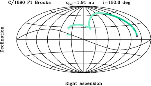
Overall view of the cometary track of C/1890 F1 Brooks from collected astrometric observations in a geocentric equatorial coordinate system given in Aitoff projection. Declination is plotted along the ordinate, and right ascension is plotted along the abscissa (increasing from zero to 360|$\circ$| from the left to right). The centre of projection is at 0|$\circ$| declination and 180|$\circ$| right ascension. The lines of right ascension and declination are shown at 30|$\circ$| intervals and the wavy line shows the projection of the ecliptic on to the celestial sphere. Each positional observation before perihelion passage is shown as a dark turquoise point, except the first observation, which is shown by a dark magenta point. The data taken after perihelion passage are marked by light turquoise points.
Global characteristics of the collected observational material are given in Table 2. The asymmetry in observed heliocentric distances around perihelion is easily visible in Fig. 2 (magenta track), where one can see that C/1890 F1 was discovered at a distance of about 2.1 au from the Sun and was followed far after the perihelion passage (1.9 au) to about 6.7 au from the Sun. In the entire data set of C/1890 F1, there are only two photographic measurements, taken by Charles Trépied on 1890 May 22 at Algiers Observatory. It is also worth noting here that Stéphane Javelle (Nice Observatory) was the only observer who followed the comet after the 7-month gap in the data due to the comet's conjunction with the Sun.
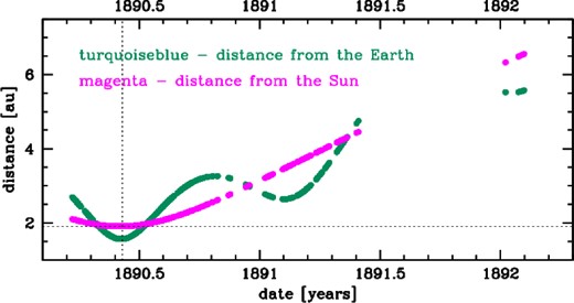
Time distribution of positional observations of C/1890 F1 Brooks with the corresponding heliocentric (magenta curve) and geocentric (turquoise curve) distances at which they were made. The horizontal dotted line shows the perihelion distance and the vertical dotted line the moment of perihelion passage.
Global description of all available astrometric observations of C/1890 F1 Brooks. Our basic set of collected data consists of 888 positional measurements that cover the same time interval as given in the fourth column (see text for an explanation).
| Comet name | qobs | T | Observational arc | No | Data | Heliocentric |
|---|---|---|---|---|---|---|
| dates | of | arc span | distance span | |||
| [au] | [yyyy mm dd.ddddd] | [yyyy mm dd – yyyy mm dd] | obs | [yr] | [au] | |
| C/1890 F1 Brooks | 1.908 | 1890 06 02.03838 | 1890 03 22 – 1892 02 05 | 908 | 1.9 | 2.11–6.56 |
3 TWO METHODS OF DATA PROCESSING
In our orbit recalculation presented here, we primarily relied on original data published by the observers. We also partially based our analysis on Strömgren's paper (1896)), where the whole set of data is published. However, we used only the -type Bordeaux observations given there, and, optionally, corrections to all 99 cometary positions in declination taken in Bordeaux since both types of data were not published anywhere else. The author received them directly from Georges Rayet, the director of Bordeaux Observatory. Therefore, to be as close to Strömgren's sample of observations as possible, our basic set of data consists of 888 positional observations, all with given -type measurements. Our full sample of data includes 20 more observations (from Washington, Vienna and Liège Observatories; see Tables 1 and 2).
The only intervention into the original data are our manual corrections of typing mistakes, which sometimes appear in published tabular data, or explicit observer errors manifesting as a kind of outlier (e.g. distant from the preliminary orbit by a whole number of minutes in right ascension or/and declination). Some of them were identified by Strömgren, often through direct contact with the observers. Thus, we took almost all of them into account and we also identified several more. The complete list of the adopted corrections can be found on our WikiComet page8 in the supplementary material to this paper.
Next, we used direct measurements of comet positions relative to reference stars, that is the -type data, to recalculate new positions of the comet using more modern star catalogues. For this purpose, we used two different approaches based on the PPM and Tycho-2 catalogues, respectively.
3.1 Method I of comet position recalculations
The first method used here is based on the reverse process to the one performed by the observers. The star's position is calculated from the measurements listed by an observer and from a given cometary position. Next, it is corrected using the PPM star catalogue (Gabryszewski 1997). Sometimes in original papers only measurements are given (in right ascension and/or in declination). When the comet's position is not given in one or both of the coordinates, we temporarily calculate the values of the missing coordinates that fit the cometary orbit, and then we look for a matching star. If successful, we obtain a position for the comet for the one or two previously unknown coordinates. This method does not require any identification of an individual reference star and its mean position, because if we can find (in the PPM star catalogue in this realization) a star within a radius of a few tens of arcseconds from the original position adopted by an observer, then we are sure in practice that this is the correct star. More details about this procedure as applied for recalculating comet positions are described by Gabryszewski (1997) and by Królikowska et al. (2014), who present the successful application of this approach to 38 Oort spike comets discovered in the first half of the 20th century.
When a certain fraction of the reference stars is successfully found for a given sample of observations, this procedure always leads to an improvement of the orbit determination by (i) a reduction of the root mean square (rms) residual and/or by (ii) enlargement of the number of applicable observations for orbit determination. Thus, it also leads to smaller uncertainties of orbital elements. Therefore, we often use this method as an effective tool for extensive studies based on large samples of comets. For this method, we decided to take a sample of 888 observations with known measurements, including the set of 99 measurements from Bordeaux. There are 38 observations where only -type data are given in the original papers, and a few dozens more for which the difference in , and as a consequence the cometary position, is given in only one coordinate (in right ascension or in declination). Since Strömgren recalculated the comet's position for almost all measurements using more modern catalogues than were previously available to the observers, it will be interesting to compare here his osculating orbit of C/1890 F1 with our orbital results based on an automatic search for reference stars in the PPM catalogue, and with the results obtained with a different re-reduction algorithm and the Tycho-2 catalogue (Section 3.2).
As we mentioned before, Strömgren published corrections to declinations for Bordeaux measurements, which he received directly from Rayet, who had observed C/1890 F1 5 yr earlier. Since the literal application of all these corrections does not seem to be obvious (see Section 3.2 for an in-depth discussion of these corrections), we divided the data into two subsets: one containing only Bordeaux measurements (subset B) and the other with all remaining observations from the basic set of 888 measurements (subset A). Next, we applied the PPM procedure to both, independently, and additionally we performed this step for two variants of subset B data. In version O, we dealt with the original measurements, whereas in version C the corrections to Δδ published in pages 32–33 of Strömgren's paper were applied. The PPM procedure gave the same results for O and C, which was expected. Namely, using the PPM procedure, corrected positions for the same 51 reference stars of the 99 original measurements were found. For subset A containing 789 observations, the reference star positions for 402 measurements were recalculated. Next, for each of the three subsets of data (each containing about 50 per cent of the recalculated cometary positions), the same sharp Bessel selection criterion was independently applied during osculating orbit determinations [for more details about our methods of data selection, see Królikowska, Sitarski & Sołtan (2009), and references therein]. The results are summarized in Table 3 and the main conclusions from these data-processing steps are as follows:
An automatic search procedure for reference stars in PPM (Gabryszewski 1997) allowed us to find new star positions for about 50 per cent of the measurements for C/1890 F1, while Strömgren found manually about 92 per cent of the stars in catalogues available to him in 1896. The difference in the effectiveness of the star search is a result not only of the manual approach applied by Strömgren, but also since the method discussed now ignores, for comparison, the data on the stars used by the observers and Strömgren. These original stellar data are used in our second method (see Section 3.2).
Table 3.Preliminary determination of an osculating orbit: comparison between original data and data recalculated using the PPM star catalogue. For the Bordeaux set of data (subset B, both versions), the selection in steps 1a and 1b was limited to the rejection of the three largest outliers. In the remaining cases, a sharp Bessel criterion was applied for data selection during orbit determination; the resulting cut-off levels (all measurements that give larger residuals are not taken into account) are displayed in columns [3], [6] and [9].
Data Number of Before PPM After PPM description measurements Step I Step II Step III (using the same limit for outliers) (repeated selection procedure) Level of Number of rms Level of Number of rms Level of Number of rms cut-off residuals cut-off residuals cut-off residuals [1] [2] [3] [4] [5] [6] [7] [8] [9] [10] [11] Subset A 789 17|${^{\prime\prime}_{.}}$|0 1380 5|${^{\prime\prime}_{.}}$|08 17|${^{\prime\prime}_{.}}$|0 1421 4|${^{\prime\prime}_{.}}$|71 14|${^{\prime\prime}_{.}}$|7 1404 4|${^{\prime\prime}_{.}}$|35 Subset B, version O 99 25|${^{\prime\prime}_{.}}$|0 197 6|${^{\prime\prime}_{.}}$|95 25|${^{\prime\prime}_{.}}$|0 198 6|${^{\prime\prime}_{.}}$|11 15|${^{\prime\prime}_{.}}$|1 193 5|${^{\prime\prime}_{.}}$|41 Subset B, version C 99 25|${^{\prime\prime}_{.}}$|0 197 5|${^{\prime\prime}_{.}}$|51 25|${^{\prime\prime}_{.}}$|0 198 4|${^{\prime\prime}_{.}}$|46 8|${^{\prime\prime}_{.}}$|9 193 3|${^{\prime\prime}_{.}}$|20 Data Number of Before PPM After PPM description measurements Step I Step II Step III (using the same limit for outliers) (repeated selection procedure) Level of Number of rms Level of Number of rms Level of Number of rms cut-off residuals cut-off residuals cut-off residuals [1] [2] [3] [4] [5] [6] [7] [8] [9] [10] [11] Subset A 789 17|${^{\prime\prime}_{.}}$|0 1380 5|${^{\prime\prime}_{.}}$|08 17|${^{\prime\prime}_{.}}$|0 1421 4|${^{\prime\prime}_{.}}$|71 14|${^{\prime\prime}_{.}}$|7 1404 4|${^{\prime\prime}_{.}}$|35 Subset B, version O 99 25|${^{\prime\prime}_{.}}$|0 197 6|${^{\prime\prime}_{.}}$|95 25|${^{\prime\prime}_{.}}$|0 198 6|${^{\prime\prime}_{.}}$|11 15|${^{\prime\prime}_{.}}$|1 193 5|${^{\prime\prime}_{.}}$|41 Subset B, version C 99 25|${^{\prime\prime}_{.}}$|0 197 5|${^{\prime\prime}_{.}}$|51 25|${^{\prime\prime}_{.}}$|0 198 4|${^{\prime\prime}_{.}}$|46 8|${^{\prime\prime}_{.}}$|9 193 3|${^{\prime\prime}_{.}}$|20 Table 3.Preliminary determination of an osculating orbit: comparison between original data and data recalculated using the PPM star catalogue. For the Bordeaux set of data (subset B, both versions), the selection in steps 1a and 1b was limited to the rejection of the three largest outliers. In the remaining cases, a sharp Bessel criterion was applied for data selection during orbit determination; the resulting cut-off levels (all measurements that give larger residuals are not taken into account) are displayed in columns [3], [6] and [9].
Data Number of Before PPM After PPM description measurements Step I Step II Step III (using the same limit for outliers) (repeated selection procedure) Level of Number of rms Level of Number of rms Level of Number of rms cut-off residuals cut-off residuals cut-off residuals [1] [2] [3] [4] [5] [6] [7] [8] [9] [10] [11] Subset A 789 17|${^{\prime\prime}_{.}}$|0 1380 5|${^{\prime\prime}_{.}}$|08 17|${^{\prime\prime}_{.}}$|0 1421 4|${^{\prime\prime}_{.}}$|71 14|${^{\prime\prime}_{.}}$|7 1404 4|${^{\prime\prime}_{.}}$|35 Subset B, version O 99 25|${^{\prime\prime}_{.}}$|0 197 6|${^{\prime\prime}_{.}}$|95 25|${^{\prime\prime}_{.}}$|0 198 6|${^{\prime\prime}_{.}}$|11 15|${^{\prime\prime}_{.}}$|1 193 5|${^{\prime\prime}_{.}}$|41 Subset B, version C 99 25|${^{\prime\prime}_{.}}$|0 197 5|${^{\prime\prime}_{.}}$|51 25|${^{\prime\prime}_{.}}$|0 198 4|${^{\prime\prime}_{.}}$|46 8|${^{\prime\prime}_{.}}$|9 193 3|${^{\prime\prime}_{.}}$|20 Data Number of Before PPM After PPM description measurements Step I Step II Step III (using the same limit for outliers) (repeated selection procedure) Level of Number of rms Level of Number of rms Level of Number of rms cut-off residuals cut-off residuals cut-off residuals [1] [2] [3] [4] [5] [6] [7] [8] [9] [10] [11] Subset A 789 17|${^{\prime\prime}_{.}}$|0 1380 5|${^{\prime\prime}_{.}}$|08 17|${^{\prime\prime}_{.}}$|0 1421 4|${^{\prime\prime}_{.}}$|71 14|${^{\prime\prime}_{.}}$|7 1404 4|${^{\prime\prime}_{.}}$|35 Subset B, version O 99 25|${^{\prime\prime}_{.}}$|0 197 6|${^{\prime\prime}_{.}}$|95 25|${^{\prime\prime}_{.}}$|0 198 6|${^{\prime\prime}_{.}}$|11 15|${^{\prime\prime}_{.}}$|1 193 5|${^{\prime\prime}_{.}}$|41 Subset B, version C 99 25|${^{\prime\prime}_{.}}$|0 197 5|${^{\prime\prime}_{.}}$|51 25|${^{\prime\prime}_{.}}$|0 198 4|${^{\prime\prime}_{.}}$|46 8|${^{\prime\prime}_{.}}$|9 193 3|${^{\prime\prime}_{.}}$|20 This recalculation of star positions significantly improved the rms of the whole data sets – compare columns [5] and [11] of Table 3. The most spectacular decrease of rms was obtained for the Bordeaux data when the Rayet corrections were applied to Δδ measurements and, as a consequence, to the original comet positions in δ for these measurements.
Rayet corrections to positions in declination appeared to improve significantly the rms at each step of orbit determination (compare columns [5], [8] and [11] for variant C and variant O).
Since Rayet's corrections to the declinations significantly reduced the scattering of data points around the orbit determined from Bordeaux measurements (these data are spread over a relatively long arc of orbit corresponding to a time interval of about 1.1 yr), we decided to construct two types of data recalculated using the PPM star catalogue:
Data Ia where Rayet's corrections were ignored
Data Ib where Rayet's corrections were applied
We used these to show how the orbit changed under the influence of these Δδ corrections suggested by Rayet for the Bordeaux measurements, which represent about 11 per cent of the whole set of data and only in declination.
At the end of this section, it is interesting to trace the relative weights of those observatories where the largest number of data points were taken. We decided to weigh the measurements according to where they were made and whether they are successfully converted using the PPM catalogue or not. Therefore, Table 4 (columns [1]–[5]) gives relative weights for subsets of original measurements, that is for those where stars were not found in the PPM catalogue (column [4]), and for subsets where stars were found and cometary positions were recalculated (column [5]). We found that for all these subsets of measurements, the recalculated parts are less dispersed around the cometary orbit than those consisting of original positions. This is manifested in higher weights in column [5] than in column [4] for each observatory given in Table 4. A spectacular improvement of the comet's position residuals is found for Pulkovo Observatory (Russia). In fact, astrometric measurements taken by Franz Renz using the 38-cm (15-inch) refracting telescope are the best in the whole data set for C/1890 F1.
Relative weights for six observatories with the largest number of measurements for three versions of data handling: Data Ib (columns [4] and [5]), Data IIa (column [6]) and Data IIb (column [7]).
| Observatory | Number | Per cent | Relative weights | |||
|---|---|---|---|---|---|---|
| location | of | of obs. | Data Ib – weighted solution | Data II – weighted solution | ||
| obs. | recalculated | original part | part of obs. | recalculated using Tycho-2 catalogue | ||
| using PPM | of obs. (star | recalculated | corr. for Bordeaux | corr. for Bordeaux | ||
| catalogue | not found in PPM) | using PPM | omitted | included | ||
| [1] | [2] | [3] | [4] | [5] | [6] | [7] |
| Bordeaux | 99 | 50.5 | 0.738 | 0.795 | 0.529 | 1.232 |
| Vienna | 78 | 62.8 | 0.515 | 0.604 | 0.630 | 0.623 |
| Hamburg | 72 | 54.2 | 0.869 | 1.031 | 1.121 | 0.821 |
| Greenwich | 62 | 48.4 | 0.422 | 0.515 | 0.372 | 0.318 |
| Kiev | 58 | 46.6 | 0.609 | 0.619 | 0.683 | 0.561 |
| Pulkovo | 54 | 66.7 | 1.458 | 3.406 | 3.874 | 3.602 |
Summarizing, Tables 3 and 4 show that the automatic search for a star's position in a modern star catalogue (here, the PPM catalogue), starting with only a comet's positions and measurements, significantly improves positional observations of comets discovered long ago.
3.2 Method II: In-depth method of comet position recalculation using the Tycho-2 catalogue
The second, partly automatic and therefore, more time-consuming method of handling positional measurements was initially inspired by the monumental work of Elis Strömgren (1896)), which has already been mentioned in previous sections. The main idea is generally the same: use only the measurements, take the mean coordinates of the reference star used by the observer and calculate a comet's position using this star position taken from the most precise source. Strömgren collected 899 observations of C/1890 F1 Brooks and compiled a list of 486 different reference stars used by observers. It seems worth mentioning that for 17 stars, Strömgren himself calculated proper motions that were unavailable at that time. On the other hand, he rejected 40 stars as having no reliable catalogue positions available to him and, as a result, he discarded 45 observations based on these stars. In his paper, he noted that an additional five observations were published after his work was completed, and in fact we found nine such additional observations, all from Vienna Observatory. We found all the original papers containing C/1890 F1 observations, except for four observations made by Dr De Baal at Liège Observatory, which Strömgren obtained in a private communication and which probably were never published separately. For these four observations, we used the data given in Strömgren's paper.
Since our aim here was to recalculate cometary positions using the -type measurements and contemporary stellar data, we excluded seven meridian circle observations made at Washington (Superintendent of USNO 1890) from this procedure. We reconstructed only the moments of these observations taken from this original communication. Additionally, a problem with Bordeaux observations also appeared: among 99 measurements only in five cases did the published data contain differences . We decided to use the differences presented by Strömgren (1896), which he reconstructed from original publications or obtained (along with the above-mentioned corrections) in the course of personal communication with Georges Rayet, the Bordeaux Observatory director at that time.
Our first step was to supply a list of mean stellar positions copied from Strömgren's list of reference stars, as a search target for the SIMBAD data base.9 Strömgren's stellar data were so good that 88 per cent of the stars were automatically found within a radius of 10 arcsec. Another 11 per cent (50 of 446 stars) were found at a distance of between 10 and 30 arcsec, and only a few stars were at distances more than 30 arcsec from the positions given by Strömgren. However, there were numerous ambiguous identifications, and of course not all of the indubitable identifications were correct, so a significant manual search and corrections were necessary. Next, we tried to identify those 40 stars for which Strömgren presented no coordinates; all of them were found in the SIMBAD data base using information given by the observers in their original papers. We also found seven additional stars used for the nine Vienna observations unavailable to Strömgren because these measurements were published after his paper was. In all, we obtained a list of 491 SIMBAD identifications of the reference stars used by C/1890 F1 observers (surprisingly, there are two stars from Strömgren's list that were not used by any observer). We were interested in the most precise astrometric parameters of these stars. About 40 per cent of them are in the Hipparcos Catalogue (Perryman et al. 1997) but due to the importance of proper motions and the necessity to use internally consistent data, we decided to use the Tycho-2 catalogue as a source for the positions and proper motions. We found Tycho-2 identifications for all 491 reference stars, and only for five of these stars were there no solutions in this catalogue (these stars are marked with the X flag indicating that there is no mean position and no proper motion), so we decided to use the positions and proper motions from the UCAC4 catalogue (Zacharias et al. 2013) for them. This addition to the Tycho stars is so small that in the remaining text, we call the stellar data source simply the Tycho-2 catalogue.
To avoid unnecessary calculations for individual observations, we introduced the following algorithm:
First, we corrected a reference star position with its proper motion from the standard epoch of J2000 to the moment of observation. These corrections were to be considered for the relatively large time interval of 110 yr and we used also parallaxes and radial velocities from the SIMBAD data base whenever they were available.
Secondly, we applied an appropriate precession matrix to express star coordinates in a mean reference frame of the epoch of observation.
Next, we added the measured
differences.At the end, we reversed the precession calculation from the second step above.
As a result, a list of 901 astrometric, topocentric positions of the comet was obtained. Moreover, they were expressed with respect to the equator and equinox of J2000 and ready for orbit determination. Such a procedure allows us to omit, for example, corrections for nutation, aberration etc. At the end we added seven meridian observations from Washington (with the epochs of observations reconstructed from local sidereal times), making the total number of observations in the Data II set equal to 908. Among them, 84 observations consisted of only one coordinate (right ascension or declination), which came to 1732 residuals potentially suitable for orbit determination.
Preliminary calculation of the O–C residuals with respect to Strömgren's orbit revealed numerous large residuals. Deep inspection of each case allowed us to eliminate most of the suspected gross errors. In this process, we confirmed most of the corrections proposed by Strömgren (see notes on pages 70 and 71 of his paper), sometimes finding different explanations. We also introduced a number of new corrections, eliminating some incorrect reference star identifications or various typos in the original papers.
As in Section 3.1, we constructed here two versions of the data [with and without corrections to Bordeaux measurements] recalculated with the Tycho-2 catalogue to study their overall influence on the resulting comet orbit:
Data IIa where corrections to Δδ of Bordeaux measurements were ignored
Data IIb where corrections to Δδ of Bordeaux measurements were applied
However, for the Data IIb set, we decided to apply corrections for Bordeaux declinations calculated from the linear model (described above) instead of those listed by Strömgren based on Rayet's estimations.
Columns 6 and 7 of Table 4 show that the Bordeaux subset of data is about 2.5 times less scattered along the orbit when these corrections for Δδ are applied. As a result, the Bordeaux Data IIb subset (column 7) has greater weights than subsets of data from Vienna, Hamburg, Greenwich or Kiev, while without these corrections, the situation is reversed.
4 NEW OSCULATING ORBIT DETERMINATIONS
In the previous section, we constructed two versions of the data for each of the two methods of data recalculation. We are convinced that the most reliable osculating orbit is based on data recalculated with the Tycho-2 star catalogue, including the corrected Bordeaux Δδ measurements according to the linear formula given by equation (1), and involving the deep data processing to eliminate as many sources of error as possible (a solution based on Data IIb).
However, to put the problem of orbit determination into a wider perspective, we constructed here a grid of osculating orbits starting from the 2 × 2 sets described in Section 3. Then, for each of them we performed two types of final data treatment during the process of orbit determination:
selection procedure based on Bessel criterion (hereafter called the A1-type solution)
selection and weighting procedure (hereafter called the A5-type solution); for our methods of data weighting see Królikowska et al. (2009) or Królikowska & Dybczyński (2010)
It should be emphasized that the process of data selection (and weighting) is individually performed for each data set and each type of model of motion (ballistic or non-gravitational), separately. In other words, it is always carried out simultaneously during the iterative process of osculating orbit determination. In this paper, we present only purely gravitational solutions (ballistic) because non-gravitational effects are very poorly determinable (the pre-perihelion branch of the orbit covered by data is distributed only over a 2-month period and the perihelion distance reaches 1.9 au; see also the very narrow range of the observed heliocentric distances before perihelion in Fig. 2). Thus, we decided not to include such uncertain solutions in the analysis presented here.
The grid of the final osculating orbits is presented in Table 5 and the O–C diagram for the Data IIb version of the observations is shown in Fig. 3. In Table 5, we omitted only two unweighted solutions for data sets constructed without the Bordeaux corrections. Nevertheless, these solutions are shown in Fig. 3 with magenta symbols. All osculating orbits given in Table 5 are of the 1A quality class using the quality class assessment of Marsden, Sekanina & Everhart (1978). However, according to a modified method that we have recently introduced (Królikowska & Dybczyński 2013), we noticed differences in quality classes: solutions based on unweighted data are of 1b class, whereas solutions based on weighted observations are of 1a class (see column [1] of the table). We consider the orbit based on the weighted data, which was previously recalculated with the Tycho-2 star catalogue with linear corrections for Bordeaux measurements of Δδ (solution A5, Data IIb), the best osculating orbit given here. Therefore, this osculating orbit was used in the analysis of the dynamical evolution of C/1890 F1 presented in Section 6. Additionally, the (O–C) distribution is Gaussian only in this case.
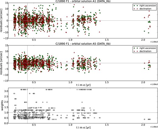
O–C diagrams for comet C/1890 F1 Brooks with the Data IIb version of observations. Two upper panels present the time distribution of positional observations with corresponding residuals based on unweighted data (orbital solution A1) and weighted data (orbital solution A5), respectively, where residuals in right ascension are shown as green dots and in declination as red triangles. The lowest panel shows relative weights for solution A5. Note that the horizontal axes show the time elapsed from the beginning of 1890 ad.
Osculating orbits of C/1890 F1 Brooks determined by Strömgren (1896) and by the present investigation. Our orbital elements of osculating heliocentric orbits are given for three alternative sets of data and two methods of further data processing. Column [1]: Epoch of osculation, type of solution (A1: unweighted data, A5: weighted data), and quality of orbit (1a or 1b) estimated using the modified method of quality assessment (Królikowska & Dybczyński 2013). [2]: Perihelion time (Terrestial Time). [3]: Perihelion distance. [4]: Eccentricity. [5]: Argument of perihelion (in degrees), equinox J2000.0. [6]: Longitude of the ascending node (in degrees), equinox J2000.0. [7]: Inclination (in degrees), equinox J2000.0. [8]: Reciprocal semi-major axis in units of 10−6 au−1. [9]: rms and number of residuals used for orbit determination. Osculating orbits determined for weighting data are indicated by light grey shading.
| Epoch [yyyymmdd] | Tobs | qobs | eobs | ωobs | Ωobs | iobs | 1/aobs | rms, |
|---|---|---|---|---|---|---|---|---|
| Type of solution | [yyyymmdd.dddddd] | [au] | [|$\circ$|] | [|$\circ$|] | [|$\circ$|] | [10−6 au−1] | Number of | |
| Quality of orbit | residuals | |||||||
| [1] | [2] | [3] | [4] | [5] | [6] | [7] | [8] | [9] |
| Osculating orbit determined by Elis Strömgren | ||||||||
| (original Rayet corrections for Bordeaux measurements of Δδ are included) | ||||||||
| 18900317 | 18900602.033026 | 1.907 583 25 | 1.000 410 30 | 68.934 397 | 320.345 283 | 120.556 094 | Strömgren (1896) | |
| Class: 1A | ±0.000447 | ±0.000 003 07 | ±0.000 013 00 | ±0.000 231 | ±0.000 096 | ±0.000 064 | Equator & equinox: 1890 | |
| 18900602 | 18900602.037500 | 1.907 582 00 | 1.000 266 00 | 68.927 300 | 321.877 900 | 120.569 000 | MWC08 | |
| Present investigation on the basis of 888 measurements and PPM star catalogue | ||||||||
| Type of data: Data Ia | ||||||||
| 18900602 | 18900602.037418 | 1.907 578 66 | 1.000 307 30 | 68.927 555 | 321.877 730 | 120.568 830 | −161.09 | 2|${^{\prime\prime}_{.}}$|94 |
| A5, class: 1a | ±0.000294 | ±0.000 002 17 | ±0.000 007 63 | ±0.000 145 | ±0.000 043 | ±0.000 047 | ±4.00 | 1591 |
| Type of data: Data Ib | ||||||||
| (original Rayet corrections for Bordeaux measurements of Δδ are included) | ||||||||
| 18900602 | 18900602.037782 | 1.907 574 11 | 1.000 278 56 | 68.927 521 | 321.877 534 | 120.568 981 | −146.03 | 4|${^{\prime\prime}_{.}}$|30 |
| A1, class: 1b | ±0.000471 | ±0.000 003 29 | ±0.000 012 51 | ±0.000 241 | ±0.000 086 | ±0.000 070 | ±6.56 | 1598 |
| 18900602 | 18900602.037418 | 1.907 578 87 | 1.000 306 40 | 68.927 548 | 321.877 721 | 120.568 824 | −160.62 | 2|${^{\prime\prime}_{.}}$|89 |
| A5, class: 1a | ±0.000291 | ±0.000 002 15 | ±0.000 007 58 | ±0.000 143 | ±0.000 043 | ±0.000 047 | ±3.97 | 1592 |
| Present investigation on the basis of 908 measurements and Tycho-2 star catalogue | ||||||||
| Type of data: Data IIa | ||||||||
| 18900602 | 18900602.037518 | 1.907 579 58 | 1.000 326 77 | 68.927 671 | 321.877 701 | 120.568 916 | −171.30 | 3|${^{\prime\prime}_{.}}$|18 |
| A5, class: 1a | ±0.000274 | ±0.000 002 00 | ±0.000 006 99 | ±0.000 133 | ±0.000 039 | ±0.000 043 | ±3.66 | 1681 |
| Type of data: Data IIb | ||||||||
| (linear corrections for Bordeaux measurements of Δδ are included) | ||||||||
| 18900602 | 18900602.038077 | 1.907 572 61 | 1.000 294 12 | 68.927 720 | 321.877 503 | 120.569 119 | −154.18 | 3|${^{\prime\prime}_{.}}$|95 |
| A1, class: 1b | ±0.000421 | ±0.000 002 92 | ±0.000 011 21 | ±0.000 217 | ±0.000 078 | ±0.000 061 | ±5.88 | 1659 |
| 18900602 | 18900602.037682 | 1.907 581 52 | 1.000 331 62 | 68.927 751 | 321.877 680 | 120.568 896 | −173.84 | 2|${^{\prime\prime}_{.}}$|61 |
| A5, class: 1a | ±0.000236 | ±0.000 001 73 | ±0.000 006 58 | ±0.000 116 | ±0.000 037 | ±0.000 037 | ±3.45 | 1644 |
Fig. 3 shows the gap in observations towards the end of the data set that stretches from 1891 May 29 to 1892 January 7 (7 months). After that gap, the comet was observed only by S. Javelle from Nice Observatory, who took nine positional measurements in the period from January 7 to February 5, as was mentioned in Section 2. At that time, the comet was more than 6 au from the Sun and more than 5.5 au from the Earth. He noted that the comet 'was extremely weak, very badly defined, and one minute wide at most’ (citation after Kronk 2013). In Fig. 3, one can see that these observations are well distributed around the orbital solution in declination. However, all measurements in right ascension give negative residuals regardless of whether the orbit was determined using unweighted (upper panel) or weighted data (middle panel, note the small weights of this set of observations). On the other hand, these measurements are very important, because they extend the period of observations by more than 8 months and thereby determine the good quality of the orbit. Apart from this trend in right ascension at the end of the data, no other systematic trends in the remaining residuals are seen in the O–C diagram based on weighted data. For the modern standards, the large scatter of residuals around the orbit based on unweighted data (upper panel of Fig. 3) draws our attention. It was, however, not unusual at that time.
Fig. 4 compares our best osculating orbit (solution A5 based on Data IIb, blue point with solid blue error bars in the figure) with the rest of the grid of osculating orbits derived here, and with Strömgren's solution given in MWC08, which is recalculated for the same epoch of 1890 June 2 (and standard equator and equinox, 2000.0) as all of our solutions discussed here (see also Table 5). This figure presents six two-dimensional projections, which indicate to what extent all these solutions are compatible. From the comparison of all the solutions shown in Fig. 4 and given in Table 5, we can draw the following conclusions:
All osculating orbits, including the solution obtained by Strömgren, are consistent within 3–4σ combined error, whereas all our weighted solutions are consistent within 1–2σ combined error (blue and red points).
 Figure 4.
Projection of the six-dimensional space of 5001 clones of C/1890 F1 on to six chosen planes of osculating orbital elements for solution A5 obtained using our best version of observations (Data IIb, i.e. recalculated using the Tycho-2 star catalogue and applying linear corrections for Bordeaux measurements of Δδ). The vertical axes of the right-hand panels are exactly the same as the vertical axes of the left-hand panels. Each grey point represents a single virtual orbit, while the large blue points with solid error bars represent the nominal weighted orbital solution for Data IIb given in Table 5. The analogous solutions derived using weighted observations in the Data Ib version are given also by blue dots inside the dotted error bars. The remaining solutions given here are shown using red dots (solutions A5: Data IIa, Data Ia), magenta squares (A1: Data IIa, Data Ia), cyan squares (A1: Data IIb, Data Ib), and green triangles, which represent the solution obtained by Strömgren. The zero-point of each axis is centred on the nominal values of the respective pair of osculating orbital elements denoted by the subscript 0 for the best solution (A5, Data IIb; see also Table 5). Error bars show 1σ errors.
The differences in orbital elements between respective pairs of solutions that differ only in ignoring or including the Δδ corrections to Bordeaux measurements are always deeply below 1σ combined error for each of the orbital elements (compare respective pairs of blue and red dots, and magenta and cyan dots). The pairs of respective orbits derived using weighted data based on the PPM catalogue (blue and red dots with dotted error bars) are closer to each other than the pairs of weighted data based on the Tycho-2 catalogue (blue and red dots with solid error bars). To understand this behaviour, we recommend analysing the weights given in Table 4 for Bordeaux observations and for different versions of the data.
The orbital element uncertainties obtained by Strömgren are very similar to those derived by us using the unweighted data (A1-type solutions, cyan and magenta error bars).
Osculating orbits based on weighted data are characterized by significantly smaller orbital element uncertainties than those given by Strömgren. He obtained his solution by using the Δδ correction for Bordeaux measurements, and somehow weighting the data when compressed into 16 normal points. Thus, we conclude that both methods used herein and based on two different modern catalogues give significantly better quality orbits.
Using the Tycho-2 catalogue to recalculate all measurements of C/1890 F1, and applying all necessary corrections, we also derived the best quality osculating orbit (solution A5, Data IIb shown in Fig. 4 as blue dots with solid error bars).
The method based on an automatic search for stars in the PPM star catalogue proposed by Gabryszewski (1997) allowed us to recalculate 50 per cent of the measurements. This also significantly improves the orbit quality and provides a solution (blue point with dotted error bars) within 2σ combined error as our best one.
5 ORIGINAL AND FUTURE BARYCENTRIC ORBITS
To be able to follow the evolution of a cometary orbit reliably, we must also know the orbital uncertainty10 at each moment of our numerical calculations. Therefore, for each solution given in Table 5, a swarm of 5001 virtual comets (VCs), including the nominal orbit, was constructed according to a Monte Carlo method given by Sitarski (1998); for more details see Królikowska et al. (2009). Next, the dynamical calculations of each swarm of VCs were performed backwards and forwards in time until each VC reached 250 au from the Sun, that is, a distance where planetary perturbations are completely negligible. This method allowed us to determine the uncertainties of the original and future orbital elements by fitting any orbital element distribution in the swarm to a Gaussian distribution at each moment of dynamical evolution.
All the original and future barycentric 1/a values are given in Table 6 whereas the full original and future orbits are presented at http://ssdp.cbk.waw.pl/LPCS and http://apollo.astro.amu.edu.pl/WCP. The distributions of these original and future swarms of 1/a are shown in Fig. 5, where the Gaussian fits to these distributions are also plotted. We conclude that the best solution (Data IIb, version A5) gives the values of 54.37 ± 3.42 and 91.18 ± 3.42, in units of 10−6 au−1, for original and future 1/a, respectively. Both are the smallest values among all respective solutions given in Table 6. Strömgren (1914) gives a value of 71.8 in the same units for original 1/a, and this value was cited by Sinding (1948), and it was taken by Oort for his famous analysis of the 1/aori distribution.
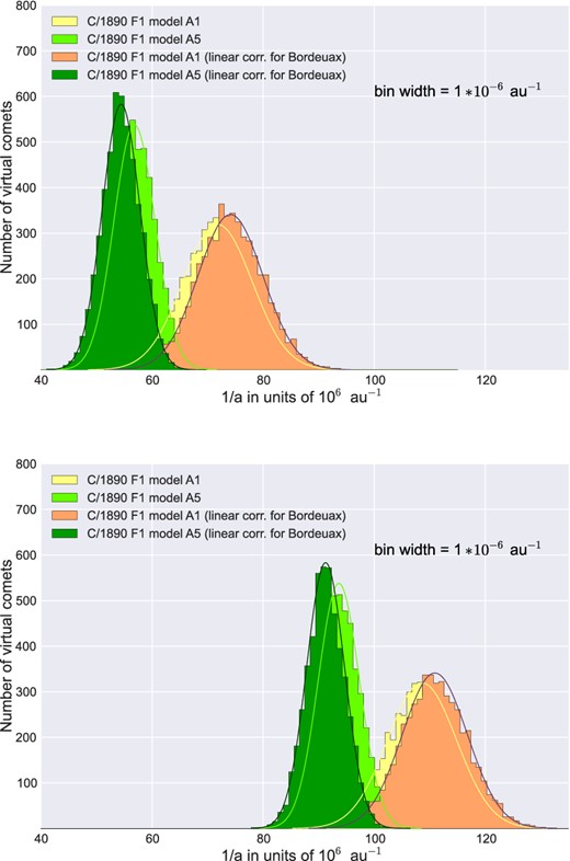
Original (upper panel) and future (lower panel) 1/a distributions for solutions based on data recalculated with the Tycho-2 catalogue. Each histogram represents the distribution of 5001 virtual comets (VCs), where the Gaussian function (continuous line) gives a perfect fit in each case. The vertical axis shows counts in each bin within the sample of 5001 clones considered in each case; this means that the counts of 500 VCs give a probability of 0.1.
Original and future barycentric inverse semi-major axes for the grid of orbital solutions of C/1890 F1. The A5 values were determined using solutions based on weighting data.
| Solution type | 1/aori | 1/afut | 1/afut − 1/aori |
|---|---|---|---|
| [au−6] | [au−6] | [au−6] | |
| Type of data: Data Ia | |||
| A1 | 79.35 ± 6.84 | 116.15 ± 6.84 | 36.796 ± 0.004 |
| A5 | 67.05 ± 3.96 | 103.85 ± 3.96 | 36.798 ± 0.002 |
| Type of data: Data Ib | |||
| A1 | 82.13 ± 6.63 | 118.93 ± 6.63 | 36.794 ± 0.004 |
| A5 | 67.60 ± 3.95 | 104.40 ± 3.95 | 36.797 ± 0.002 |
| Type of data: Data IIa | |||
| A1 | 71.77 ± 6.25 | 108.59 ± 6.24 | 36.802 ± 0.004 |
| A5 | 56.91 ± 3.71 | 93.71 ± 3.71 | 36.803 ± 0.002 |
| Type of data: Data IIb | |||
| A1 | 74.02 ± 5.85 | 110.82 ± 5.85 | 36.800 ± 0.003 |
| A5 | 54.37 ± 3.42 | 91.18 ± 3.42 | 36.805 ± 0.002 |
The mutual proximity of swarms A1 and A5 obtained using Tycho-2 (Data IIb) in a two-dimensional projection is visualized in Fig. 6. We can find a similar overlapping of the swarms in every other projection.
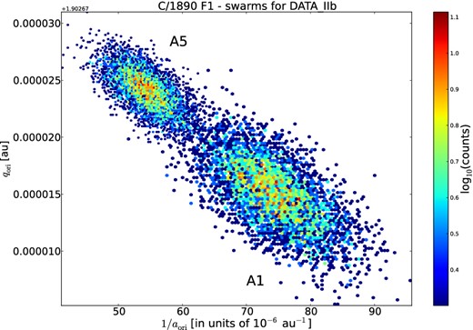
Projection of two original swarms of 5001 VCs (six dimensions each) of C/1890 F1 Brooks on to the 1/a versus q plane. These swarms represent solutions derived from the Data IIb type of data, where the less dispersed swarm (upper left, and given by the dark green histogram in Fig. 5) represents the A5 solution based on data that were weighted during the procedure of orbit determination, whereas the more disperse swarm shows the A1 solution (given by the sandy brown histogram in the upper left-hand panel of Fig. 5). The density distribution of the A5 swarm is superimposed on that of the more dispersed A1 swarm. The density map is given in logarithmic scale, which is presented in the individual panel on the right. Note that the value of the beginning of the vertical axis is given just above the upper horizontal border of the plot.
Note that C/1890 F1 is very interesting from the point of view of planetary perturbations: it suffered very small perturbations from planets during its passage through the planetary zone in the observed 1890–1892 apparition. Regardless of the version of the data used, these perturbations are at the level of δ(1/a) = 1/afut − 1/aori ≃ 36.8 × 10⁻⁶ au−1 (last column of Table 6). As a result, according to the best solution, the comet will still be inside the Oort spike in the next apparition.
Table 7 gives other examples of comets that were subjected to weak planetary perturbations. All were selected from the sample of about 160 Oort spike comets investigated by us so far. Here, we present only comets with a small perihelion distance of qobs < 3.5 au, just as we have done for comet C/1890 F1. However, we have also recognized another 25 objects of that kind with large qobs, which constitute a significant percentage of these large perihelion objects (for more details, see discussion in Dybczyński & Królikowska 2011). Otherwise, the 13 comets presented here (12 from Table 7 plus C/1890 F1) make up only about 15 per cent of the small perihelion Oort spike comets. Among them, five objects have orbits almost perpendicular to the ecliptic plane and move on retrograde orbits; these are shown using asterisks in Table 7. When we further reduce the sample to comets that have passed to a more bound orbit during the passage through the planetary zone, we find only six such cases. Therefore, we can say that because it suffers such small planetary perturbations, the dynamical behaviour of C/1890 F1 is unusual among small perihelion comets.
Original and future barycentric inverse semi-major axes and their Δ1/a = 1/afut − 1/aori differences for other Oort spike comets subjected to weak planetary perturbations during the observed perihelion passage through the planetary zone (|Δ1/a| < 100 in units of 10−6 au−1). Only comets with a perihelion distance closer than 3.5 au to the Sun are presented here. Original and future 1/a values were taken from Królikowska (2014) and Królikowska et al. (2014). Comets with an inclination to the ecliptic inside the range 80|$\circ$|–100|$\circ$| (all on retrograde orbits, see column [7]) are indicated by an asterisk.
| Comet | 1/aori | 1/afut | Δ(1/a) | 1σ error | Quality | qobs | iobs |
|---|---|---|---|---|---|---|---|
| [au−6] | [au−6] | [au−6] | [au−6] | class | [au] | [|$\circ$|] | |
| [1] | [2] | [3] | [4] | [5] | [6] | [7] | |
| C/1913 Y1 Delavan | 52.57 ± 4.23 | 86.84 ± 4.23 | +34.27 | <0.01 | 1a | 1.1 | 68.2 |
| C/1919 Q2 Metcalf | 34.7 ± 67.3 | −26.9 ± 67.3 | −61.56 | 0.05 | 2a | 1.1 | 46.4 |
| C/1946 P1 Jones | 50.86 ± 5.08 | 22.55 ± 5.08 | −28.32 | <0.01 | 1a | 1.1 | 57.0 |
| C/1946 U1 Bester | 17.08 ± 6.52 | 43.88 ± 6.52 | +26.80 | <0.01 | 1b | 2.4 | 108.2 |
| C/1947 Y1 Mrkos | 28.89 ± 8.49 | 54.31 ± 8.50 | +25.42 | <0.01 | 1b | 1.5 | 77.5 |
| C/1948 E1 Pajdušáková-Mrkos* | 37.25 ± 2.74 | 35.21 ± 2.74 | −2.04 | <0.01 | 1a | 2.1 | 92.9 |
| C/1952 W1 Mrkos* | −0.1 ± 85.8 | −41.4 ± 106.9 | −40.6 | 43.3 | 2a | 0.8 | 97.2 |
| C/1989 Q1 Okazaki-Levy-Rudenko* | 42.9 ± 22.2 | 80.5 ± 27.3 | +37.6 | 46.6 | 2a | 0.6 | 90.1 |
| C/1997 J2 Meunier-Dupouy* | 44.64 ± 0.88 | 14.72 ± 0.91 | −29.92 | 1.47 | 1a+ | 3.1 | 91.3 |
| C/2006 HW51 Siding Spring | 47.31 ± 3.37 | 90.12 ± 3.37 | +42.81 | <0.01 | 1a | 2.3 | 45.8 |
| C/2006 S2 LINEAR* | 72.52 ± 8.14 | −10.77 ± 18.09 | −83.3 | 25.5 | 1b | 3.2 | 99.0 |
| C/2007 Q3 Siding Spring | 39.13 ± 0.49 | 118.96 ± 0.96 | +79.83 | <0.01 | 1a+ | 2.3 | 65.7 |
6 PREVIOUS AND NEXT PERIHELION PASSAGES
With the original and future barycentric orbits, we can study the past and future motion of C/1890 F1 Brooks by following its motion numerically. At distances greater than 250 au, we ignore all planetary perturbations but we include Galactic and stellar perturbations and integrate the comet motion to the previous and next perihelion passage, that is about 2.5 Myr in the past and 1.1 Myr in the future. Since the previous and next perihelion passages of C/1890 F1 are deep in the planetary zone and we cannot calculate planetary perturbations at these epochs, we have to stop our calculations at these moments. Of course, for that reason, one should treat our previous orbit as the osculating one when the comet left the planetary zone after the previous perihelion. Analogously, one should treat the next orbit as the osculating one before the comet will enter the planetary zone during its next apparition.
In this investigation, we used exactly the same dynamical model as in Paper V. It includes Galactic disc and Galactic Centre tidal terms and perturbations from 90 stars or stellar systems known to have passed closer than 3.5 pc from the Sun in the past, currently or in the future. Since we study the motion of C/1890 F1 in an interval smaller than 4 Myr, these stellar data can be considered complete in terms of massive and slow moving perturbers; see Paper V for a detailed discussion and a description of the stellar perturbers. Stellar perturbers, together with a comet, are numerically integrated as an N-body problem in the Solar system barycentric frame with additional Galactic tidal potential. This calculation has been repeated for the nominal orbit of this comet and for all 5000 VCs to propagate observational uncertainties.
The past and future motion of C/1890 F1 is quite regular and all previous and next orbital clones move on elliptical orbits in each of the analysed swarms. The most important parameters of these orbits are given in Table 8. We present here the results of two different calculations – with and without stellar perturbations – to show how small their influence is. In contrast to the almost perfectly normal distributions of the inverse semi-major axes in all of the analysed solutions, the perihelion and aphelion distances have non-Gaussian distributions (see also their histogram below). Therefore, in Table 8, we describe the distribution of qprev, qnext, Qprev and Qnext by presenting their median values accompanied with 10th and 90th deciles.
C/1890 F1 previous and next orbital parameters derived from the Data IIb set of observations. The inverse semi-major axis is presented as the Gaussian mean value and its 1σ uncertainty. Tprev and Tnext are the epochs of the previous and next perihelion, respectively. The perihelion and aphelion distances, as well as their epochs, are presented as 10th:50th (the median):90th deciles due to departure of their distributions from a normal one. Solution names subscripted with a star means that all known stellar and Galactic perturbations were included in the numerical integrations, in contrast to the solutions without subscripts, where only Galactic perturbations were included.
| Solution | Tprev | 1/aprev | qprev | Qprev | Tnext | 1/anext | qnext | Qnext |
|---|---|---|---|---|---|---|---|---|
| [Myr] | [10−6au−1] | [au] | [103au] | [Myr] | [10−6au−1] | [au] | [103au] | |
| A5* | −2.81:−2.48:−2.20 | +54.44 ± 3.42 | 3.17:3.64:4.35 | 34.0:36.8:40.0 | 1.07:1.15:1.24 | +91.24 ± 3.42 | 1.65:1.69:1.72 | 20.9:21.9:23.0 |
| A5 | −2.81:−2.48:−2.20 | +54.44 ± 3.42 | 3.09:3.53:4.20 | 34.0:36.8:40.0 | 1.07:1.15:1.24 | +91.24 ± 3.42 | 1.65:1.69:1.72 | 20.9:21.9:23.0 |
| A1* | −1.83:−1.56:−1.35 | +74.17 ± 5.85 | 2.27:2.42:2.67 | 24.5:27.0:30.0 | 0.78:0.86:0.96 | +110.91 ± 5.85 | 1.76:1.79:1.81 | 16.9:18.0:19.3 |
| A1 | −1.83:−1.56:−1.35 | +74.12 ± 5.85 | 2.25:2.40:2.64 | 24.5:27.0:30.0 | 0.78:0.86:0.96 | +110.92 ± 5.85 | 1.76:1.79:1.82 | 16.9:18.0:19.3 |
As was highlighted in Section 5, comet C/1890 F1 Brooks suffered only small planetary perturbations during its observed perihelion passage. Looking at a wider perspective, we see that it was observed in a decreasing phase of the evolution of its perihelion distance due to the Galactic tides. The perihelion distance decreases from qprev = 3.64 au through qobs = 1.91 au down to qnext = 1.69 au. Taking into account only shortening of the small semi-major axis by planetary perturbations, C/1890 F1 is an example of an Oort spike comet visiting the deep interior of the Solar system (and therefore, being observable) in at least three consecutive perihelion passages, while still being a member of the spike. This behaviour is clearly shown in Fig. 7.
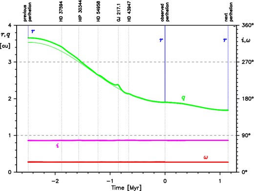
Past and future evolution of the nominal orbit of C/1890 F1 for the preferred solution under simultaneous Galactic and stellar perturbations.
Many interesting aspects of the past and future orbital evolution of C/1890 F1 under stellar and Galactic perturbations can be found in Fig. 7. In this picture, the horizontal time axis extends from the previous perihelion passage through the observed apparition up to the next perihelion passage. The left vertical axis is in astronomical units and describes the osculating perihelion distance evolution (q, green line), as well as the heliocentric distance plot (r, thin blue lines). Due to the time-scale of this picture, the heliocentric distance plots take the form of vertical blue lines exactly at perihelion passage moments. The right vertical axis is expressed in degrees and describes changes in the osculating inclination (i, magenta line) and in the argument of perihelion (ω, red line). Both of these angular elements are expressed in the Galactic frame. All thick lines depict dynamical evolution under joint stellar and Galactic perturbations, while the thin lines mark the evolution with the stellar perturbations excluded. Horizontal dashed lines draw attention to the beginning of the second and fourth quarter of ω, whose values (90|$\circ$| and 270|$\circ$|) are important from the point of view of the Galactic perturbations (crossing these lines coincides with a perihelion distance minimum). The vertical dashed lines show the closest approaches of the comet to a star or stellar system, the name of which is at the top of the picture. It is worth mentioning that the timing of a stellar perturbation is not necessarily strictly aligned with this closest approach moment – it strongly depends on the geometry, since the final heliocentric orbit change is a net effect of stellar gravitational action on both the comet and the Sun. The action of GJ 217.1 is a good example of a frequent self-cancelling stellar action: the perturbation gained during the approaching phase is then cancelled during the receding phase. During the presented 3.5-Myr interval of cometary evolution, the Galactic and stellar perturbations are notable only in the perihelion distance, while being infinitesimally small in angular elements. We have not identified any profound stellar perturbation in the future motion of C/1890 F1 since it will depart from the Sun for only about 20 000 au and it will complete its future orbital revolution (1.1 Myr) about 0.3 Myr before the predicted close flyby of the star Gliese 710. Other stars are too small and/or too distant to noticeably change the future orbit of this comet.
C/1890 F1 is definitely a dynamically old comet. Even the most protruding clones in our swarm of VCs have a previous perihelion distance well below 10 au. The osculating perihelion distance and the inverse semi-major axis distributions of C/1890 F1 for the moment of the previous perihelion passage (nominally 2.5 Myr ago) are presented in Fig. 8. It is worth mentioning that the presented 1/a distribution is still almost perfectly Gaussian while the q distribution significantly departs from the normal one, mainly as a result of Galactic perturbations. The central, black joined distribution corresponds to the smaller cloud of 5001 VCs presented in Fig. 6 after 1.7–3.8 Myr of backward dynamical evolution under simultaneous Galactic and stellar action (different VCs have different orbital periods, a nominal value equals 2.5 Myr, the fastest VC was at the previous perihelion 1.7 Myr ago while the slowest one almost 3.8 Myr ago).
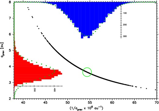
Joint and marginal distributions of the osculating 1/a and q of 5001 VCs derived from the nominal orbit of the preferred solution for C/1890 F1, stopped at their previous perihelion passage. The centre of the green circle marks the nominal values. Small green dots overprinted on the marginal distributions show best-fitting Gaussian distributions.
The time-spread (along the horizontal axis) and the space-spread (along the vertical axis) of our swarms of VCs for the previous and next perihelia are clearly visualized in Fig. 9. We presented here changes in the barycentric distance of all 5001 VCs from two different solutions of orbit determination, both based on the Data IIb set of observations. The red (darker) swarm depicts the distribution evolving from the osculating orbit fitted to the weighted observations (A5 solution) while the green (grey) one depicts the evolution of the swarm constructed without weighting (A1 solution). Nominal orbits for both of our solutions are marked as black curves. Thus, this figure shows also how the data handling can change the results during the evolution to the previous/next perihelion distance (see also Table 8). The dynamical evolution of Strömgren's orbit would be very similar to the evolution of our A1 orbital solution. We conclude that our preferred A5 solution gives longer previous and next orbital periods of about 2.5 and 1.1 Myr, respectively. As a result, Galactic perturbations are more effective during the evolution, and for this solution we get a greater change of the perihelion distances between the three consecutive perihelion passages analysed here.
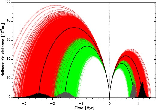
Past and future swarms of C/1890 F1 orbits for two different solutions based on the Data IIb set of observations: red (dark grey) lines represent results for the A5 solution (preferred, weighted data) while green (light grey) lines correspond to the A1 solution (without data weighting, see Tables 6 and 8 for more details). All known stellar and Galactic perturbations were taken into account. Black lines depict the evolution of nominal orbits. The distributions of previous and next perihelion epochs are also shown.
7 SUMMARY AND CONCLUSIONS
The rich observational material for C/1890 F1 Brooks allows us to test whether it is productive to recalculate the original positions of comets discovered long ago using modern star catalogues. During this study we compared two distinct algorithms:
an automatic search for reference stars in the PPM star catalogue according to Gabryszewski (1997), which was frequently used by us when we have only
 measurements and data on the positions of comets.
an automatic search for reference stars in the Tycho-2 star catalogue on the basis of mean coordinates of reference stars used by all observers, and next, a detailed analysis of all the cases of large residuals in the observed cometary positions, resulting from the star search (∼30 per cent of all observations for C/1890 F1).
The first method has been successfully used several times before, more recently by Królikowska et al. (2014). This method of automatically searching for stars in the PPM catalogue recalculates about 50 per cent of the existing data of C/1890 F1. The second method was developed for the present investigation. We successfully found in the SIMBAD data base all the stars used by the observers more than a hundred years ago to calculate the comet's position in α and/or δ from measurements. This means that all positions of C/1890 F1 were recalculated here using these original measurements (Δα and/or Δδ). We decided to use stellar positions and proper motions from the Tycho-2 catalogue for that purpose.
It should be emphasized that thanks to the monumental publication by Elis Strömgren (1896), our task is much easier, though it was still time-consuming. Searching for stars in the SIMBAD data base would be more difficult without the mentioned publication, particularly in the more complicated cases. In addition, thanks to Strömgren's deep analysis of the data, it turned out that one should take into account corrections to Δδ measurements from Bordeaux Observatory (we prefer a linear version of these corrections as described in Section 3.2). However, these corrections change the orbital solution on a significantly lower level than the use of modern stellar data. For example, a solution based on data recalculated in about 50 per cent (PPM catalogue, Data Ia/Data Ib) differs substantially from the respective solution based on fully recalculated data (Tycho-2 catalogue Data IIa/Data IIb) than any two solutions based on data with and without Bordeaux corrections. Moreover, the Bordeaux corrections are also much less important than the method of data treatment. This is clearly shown in Fig. 5, where we can see that the light green histogram (weighted data, corrections for Bordeaux omitted) is very similar to the dark green histogram (weighted data, corrections for Bordeaux applied); however, it differs significantly from the pair of yellow and orange histograms based on unweighted data.
We have shown that both search algorithms for contemporary data for the reference stars resulted in a significant reduction of the uncertainties of orbital elements for C/1890 F1 Brooks. A comparison of our solutions with that derived by Strömgren is presented in Table 5 and Fig. 4. By analysing all these models, we concluded that the orbital solution based on Data IIb (all positional observations were recalculated using the Tycho-2 catalogue and then weighted) gives the most reliable and also the most accurate osculating orbit.
Using this most preferred orbital solution (and its unweighted variant for comparison, see Fig. 9), we numerically followed the motion of C/1890 F1 for one orbital period in the past and in the future. Starting from full swarms of original and future VC orbits, we obtained the previous and next orbital elements of this comet together with their uncertainties. All known stellar and Galactic perturbations were fully taken into account but for the comparison, we also performed calculations in which stellar perturbations were ignored. This comparison (see Table 8 for details) shows that none of the known stellar perturbers significantly change the past and future motion of C/1890 F1 during the three successive perihelion passages analysed here. It should be stressed that due to the relatively short past orbital period of C/1890 F1 Brooks (nominally 2.5 Myr), it seems rather improbable that we have missed here some unknown but significant (i.e. massive and/or slow moving) and nearby stellar perturber.
The three consecutive perihelion passages of this comet (a time interval of about 3.6 Myr) clearly indicate that this comet deeply penetrates the planetary region during each of them (less than 5 au from the Sun, see Table 8) and it easily crosses the so-called Jupiter–Saturn barrier. Therefore, we conclude that C/1890 F1 Brooks is a dynamically old comet and additionally, as a result of negligible planetary perturbations during the observed apparition, it will remain a member of the Oort spike during the next apparition. Note that Oort (1950) treated this comet (by definition) as a dynamically new one and used it in support of his cometary cloud hypothesis.
Currently, from the analysis of 109 Oort spike comets, we estimate that about 50 per cent of them are dynamically old. However, the percentage of dynamically old comets grows to almost 90 per cent for comets with 1/aori inside the range of 0.000 040–0.000 100 au−1 (Paper V). Thus, the past dynamical evolution of comet Brooks having 1/aori greater than 0.000 050 au−1 is not surprising. On the other hand, due to the very weak planetary perturbations, one can say that the dynamical behaviour of C/1890 F1 is unusual among small perihelion comets.
In the near future, we plan to deal with all near-parabolic comets discussed by Oort (1950) as well as all Oort spike comets discovered during 1901–1950 to determine their source from a previous perihelion perspective and to make our sample of near-parabolic comets with known previous and next orbital elements more complete. Possibly, some comets observed on a more tightly bound orbit (1/aobs > 0.000 100 au−1) will contribute to a future 1/a distribution as Oort spike comets. Therefore, the extension of our research to objects with 1/a like that of C/2013 V2 Borisov [1/aori = 0.000 770 au−1 and 1/afut = 0.000 089 au−1, Nakano (2015)] seems to be important for putting our investigation in the broader framework of the dynamical evolution of long-period comets.
Some auxiliary material to this paper is available at http://ssdp.cbk.waw.pl/LPCS and http://apollo.astro.amu.edu.pl/WCP.
We are very grateful to Ryszard Gabryszewski for providing software and related assistance with the search for stars in the PPM star catalogue. We also thank the anonymous referee of this paper for valuable remarks. This research made use of NASA's Astrophysics Data System Bibliographic Services and the SIMBAD data base and VizieR catalogue access tool, CDS, Strasbourg, France (Wenger et al. 2000), and was partially supported by the project 2015/17/B/ST9/01790 founded by the National Science Centre in Poland.
Comet–star measurements.
This is always the starting nominal orbit for our numerical calculations of dynamical evolution.
Large sets of such data were typed into computer files during a long campaign of collecting observations of one-apparition comets as a part of the Warsaw Catalogue of Cometary Orbits project (Królikowska et al. 2014).
After his investigation, nine more measurements taken in Vienna were published and these are also included in our orbit determination using the Tycho-2 star catalogue.
This results from the observational uncertainty of the osculating orbit; see Table 5.
REFERENCES
