


Abstract
We use a damped mass-spring model within an N-body code to simulate the tidal evolution of the spin and orbit of a self-gravitating viscoelastic spherical body moving around a point-mass perturber. The damped mass-spring model represents a Kelvin–Voigt viscoelastic solid. We measure the tidal quality function (the dynamical Love number k2 divided by the tidal quality factor Q) from the numerically computed tidal drift of the semimajor axis of the binary. The shape of k2/Q, as a function of the principal tidal frequency, reproduces the kink shape predicted by Efroimsky for the tidal response of near-spherical homogeneous viscoelastic rotators. We demonstrate that we can directly simulate the tidal evolution of spinning viscoelastic objects. In future, the mass-spring N-body model can be generalized to inhomogeneous and/or non-spherical bodies.
1 MOTIVATION AND PLAN
The analytical theory of tidal interaction of solid bodies has a long and rich history – from the early mathematical development by Darwin (1879),1 to its generalization by Kaula (1964), to an avalanche of more recent results. Verification of tidal theories through direct measurements is not easy because the tidal evolution is slow and requires either high observational precision (Williams & Boggs 2015) or an extended observational time span (Lainey et al. 2012). Purely analytical theories of tidal evolution describe homogeneous or, at best, two-layered (as in Remus et al. 2015) near-spherical bodies of linear rheology. This makes numerical simulations attractive (e.g. Henning & Hurtford 2014) as they may make it possible to explore the tidal evolution of more complex objects.
Here we explore computations that treat the solid medium as a set of mutually gravitating massive particles connected with a network of damped massless springs. Because of their simplicity and speed (compared to more computationally intensive grid-based or finite element methods), mass-spring computations are a popular method for simulating soft-deformable bodies (e.g. Nealen et al. 2006). Ostoja-Starzewski (2002) and Kot, Nagahashi & Szymczak (2015) have shown that mass-spring systems can accurately model elastic materials. As we shall show, viscoelastic response and gravitational forces can be incorporated into the mass-spring particle-based simulation technique. We demonstrate numerical simulations of the tidal response of a spinning homogeneous spherical body exhibiting spin-down or spin-up and associated drift in semimajor axis, without using an analytical tidal evolution model. Then we compare the outcome of our numerics with analytical calculations. The results are similar, justifying our numerical approach. Our numerical model may in future be used to take into account more complex effects that cannot be easily computed by analytical means (like inhomogeneity, compressibility, or a complex shape of the tidally perturbed body).
2 TIDES IN A KELVIN–VOIGT VISCOELASTIC SOLID
2.1 How tides work
2.2 The shape of the quality function
As is demonstrated in Appendix A, the Fourier decompositions of the disturbing potential W, the tidal response potential U, and the tidal torque |${\cal {T}}$| comprise terms that are numbered with the four indices lmpq. An lmpq term of the torque is proportional to the quality function kl(ωlmpq) sin ϵl(ωlmpq). The quality function depends on the degree l, the composition of the body, the rheology of its layers, and the size and mass of the body. The size and mass are important, because the tidal response is defined not only by the internal structure and rheology, but also by self-gravitation.
The generic shape of the quality function can be understood by comparing the frequency χ to the inverse of the viscoelastic relaxation time (e.g. Ferraz-Mello 2015b.). At a fixed point in the body, the tidal stressing in the material is oscillating at the frequency χ ≡ |ω|. When χ is small compared to the inverse time-scale of viscoelastic relaxation in the material, the body deformation stays almost exactly in phase with the tidal perturbation. The reaction and action being virtually in phase, no work is carried out and the tidal effects are minimal. On the other hand, at very high frequencies, the body's viscosity prevents it from deforming during the short forcing period 2π/χ. The reaction cannot catch up with the action, and stays close to zero – so, once again, little work is being done, and the tidal effects are again minimal.
2.3 The quality function for a Kelvin–Voigt sphere
The goal of our paper is not to favour a particular rheological model, but to test our simulation method. The Kelvin–Voigt rheological model is simplistic,4 but it is the easiest to model with a mass-spring model. Subsequent work will be aimed at extending our simulation approach to more realistic rheologies.
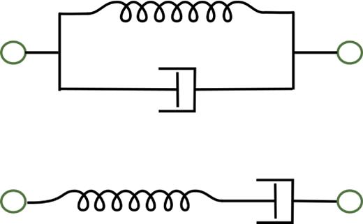
Green circles are mass elements. In the Kelvin–Voigt model (the top drawing), spring and damping elements are set in parallel. In the Maxwell model (the bottom drawing), the two elements are arranged in series. Since it is easier to represent a Kelvin–Voigt viscoelastic material with a mass-spring network, we compute the quality function for the Kelvin–Voigt model, thus allowing a direct comparison between the quality functions calculated from theory and that computed through simulation.
Classical tidal theory is valid only for incompressible materials (those having the Poisson ratio ν = 0.5) – which is why the standard expression for the static Love number k2 of an incompressible sphere depends only on the shear modulus of rigidity, not on the bulk modulus. However, the mass-spring models approximate a material with Poisson's ratio ν = 0.25 (Kot et al. 2015). However, Love (1911) derived a general formula for the static Love number k2 also for a compressible homogeneous sphere.5 We have numerically checked that his formula for k2 in the compressible case is only very weakly dependent on the Poisson's ratio, within broad ranges of the body size and density. This makes us confident that the standard tidal formulae (derived for the Poisson ratio ν = 0.5) can accurately describe a compressible body with Poisson ratio ν = 0.25.
3 DAMPED MASS-SPRING MODEL SIMULATIONS
We will compare the tidal spin-down rate of a simulated viscoelastic body to that predicted analytically. To simulate tidal viscoelastic response we use the mass-spring model by Quillen et al. (2015), that is based on the modular N-body code rebound (Rein & Liu 2012). A random spring network model, rather than a lattice network model, was chosen so that the modelled body is approximately isotropic and homogenous and lacks planes associated with crystalline symmetry. We work in units of radius and mass of the tidally perturbed body: R = 1, M = 1. Time is given in units of |$t_{{\rm grav}} = \sqrt{R^3/GM\,}$| referred to as the gravitational time-scale. Pressure, energy density, and elastic moduli are specified in units of eg ≡ GM2/R4. In these units, the velocity of a massless particle on a circular orbit, which is just grazing the surface of the body, is 1, the period of the grazing orbit being 2π.
Modelling the tidally perturbed body, we randomly generate an initial spherical distribution of particles of equal mass (as described in section 2.2 in Quillen et al. 2015); see our Fig. 2 for an illustration. Particle positions are randomly generated using a uniform distribution in three dimensions but a particle is added (as a node) to the spring network only if it is sufficiently separated from other particles (at a distance greater than minimum distance dI) and within a radius of R = 1 from the body centre. Springs are added between two nodes if the distance between the nodes is less than distance ds.
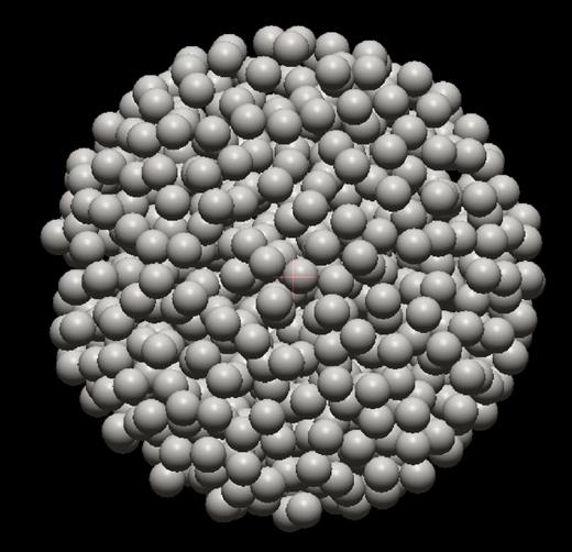
A snapshot of one of our simulations as viewed in the open-GL viewer of rebound. We only show the tidally perturbed body, as the perturbing one is distant from it. The rendered spheres are shown to illustrate the random distribution of node point masses, not imply that the body behaves as a rubble pile (e.g. Richardson et al. 2009; Sánchez & Scheeres 2011). Nodes are connected with a network of damped elastic springs.
The particles are subjected to three types of forces: the gravitational forces acting on every pair of particles in the body and with the massive companion, and the elastic and damping spring forces acting only between sufficiently close particle pairs. Springs with a spring constant kI interconnect each pair of particles closer than some distance ds. The rest length of each spring is initially set equal to its initial length. The springs experience compression or extension relative to their rest length. The number of springs and their rest lengths stay fixed during our simulations. The springs have different rest lengths, and we denote their average initial (rest) length with LI. The total number of particles is NI, and the total number of springs is NSI. The mass of each particle is mI = 1.0/NI, and the initial mass density is approximately uniform.
The number and distribution of particles and links in a mass-spring model is mainly set by the minimum distances dI, ds, however, because the initial particle positions are randomly generated, there are local variations in density of nodes and the spring network. The ratio ds/dI sets the mean number of springs per mass node.
From the rebound code, version 2 as of 2015 November, we used the open-GL display with open boundary conditions, the direct all-pairs gravitational force computation, and the leap-frog integrator needed to advance particle positions. To the particles’ accelerations caused by the gravity, we added the additional spring and spring-damping forces, as was explained above. To maintain numerical stability, the time step was chosen to be smaller than the elastic oscillation frequency of a single node particle in the spring network, or equivalently the time it takes vibrational waves to travel between two neighbouring nodes.
4 TIDAL EVOLUTION OF THE SEMIMAJOR AXIS
4.1 The semimajor axis’ tidal drift rate computed from the mass-spring model
Common parameters for our first set of simulations are listed in Table 1, along with their chosen or computed values. A list of varied and measured parameters is presented in Table 2. The values used in different individual simulations with common values in Table 1 are listed in Table 3. We chose the values for the mass ratio M*/M and the initial semimajor axis a0 to be the same in the two sets of simulations performed. However, in each set, the spring damping rate γI and the initial body spin rate σ0 were chosen to sample a range of values of the Fourier tidal mode frequency ω and of the viscoelastic relaxation time τrelax. Using the equation (29), we computed the Young's modulus by only considering the springs with a midpoint radii less than 0.9R, and we used the volume within the same radius 0.9R. The region near the surface was discarded so that the Young's modulus was computed in a region where the spring network is isotropic. A fairly soft body under strong tidal forcing (corresponding to a large mass ratio and weak springs) was chosen, to reduce the integration time required to observe a significant tidally induced change in the semimajor axis. At the same time, we made sure that the Young's modulus was sufficiently large, so that the body was strong enough to maintain a nearly constant radial density profile. In the absence of exterior pressure, the body is held up against self-gravity by spring forces only – so the springs in the interior are under compression. In all our runs, the particles were displaced, in the body frame, by at most a few per cent of the unit length R.
Common simulation parameters.
| NI | 800 | Number of particles in resolved body |
| NSI | 9254 | Number of interconnecting springs |
| LI | 0.2623 | Mean rest spring length |
| kI | 0.08 | Spring constant |
| EI | 2.3 | Mean Young's modulus |
| dI | 0.15 | Minimum initial interparticle distance |
| ds | 0.345 | Spring formation distance |
| dt | 0.001 | Time step |
Description of varied and measured simulation parameters.
| a0 | Initial semimajor axis |
| M*/M | Mass ratio |
| |$\tilde{\chi }$| | Unitless frequency |
| |$\dot{a}$| | Rate of orbital decay in semimajor axis |
| γI | Spring relaxation time |
| σ0 | Initial spin |
| τrelax | Estimated relaxation time of viscoelastic solid |
| χ | Initial tidal frequency (semidiurnal) |
| Po | Time between integration outputs |
| EI | Computed Young's modulus |
Quantities either set or computed in different mass-spring N-body simulations.
| |$\tilde{\chi }$| | |$\dot{a}$| | γI | σ0 | τrelax | χ | Po | EI |
|---|---|---|---|---|---|---|---|
| With a0 = 10, M* = 100, n = 0.318 | |||||||
| 0.069 | −3.897e-05 | 20 | 0.1 | 0.158 | 0.436 | 14.424 | 2.30 |
| 0.162 | −8.505e-05 | 20 | −0.2 | 0.156 | 1.036 | 6.067 | 2.35 |
| 0.223 | −1.055e-04 | 20 | −0.4 | 0.156 | 1.436 | 4.377 | 2.40 |
| 0.447 | −1.800e-04 | 40 | −0.4 | 0.311 | 1.436 | 4.377 | 2.38 |
| 0.645 | −2.309e-04 | 50 | −0.5 | 0.394 | 1.636 | 3.841 | 2.33 |
| 0.896 | −2.517e-04 | 80 | −0.4 | 0.624 | 1.436 | 4.377 | 2.36 |
| 1.123 | −2.288e-04 | 100 | −0.4 | 0.782 | 1.436 | 4.377 | 2.36 |
| 1.467 | −2.325e-04 | 100 | −0.6 | 0.799 | 1.836 | 3.423 | 2.26 |
| With a0 = 20, M* = 200, n = 0.159 | |||||||
| 0.080 | −2.239e-06 | 20 | −0.1 | 0.156 | 0.517 | 12.153 | 2.40 |
| 0.160 | −4.540e-06 | 40 | −0.1 | 0.309 | 0.517 | 12.153 | 2.41 |
| 0.227 | −7.124e-06 | 40 | −0.2 | 0.317 | 0.717 | 8.763 | 2.29 |
| 0.350 | −8.601e-06 | 40 | −0.4 | 0.314 | 1.117 | 5.625 | 2.36 |
| 0.534 | −1.157e-05 | 60 | −0.4 | 0.478 | 1.117 | 5.625 | 2.25 |
| 0.701 | −1.324e-05 | 80 | −0.4 | 0.627 | 1.117 | 5.625 | 2.26 |
| 0.881 | −1.656e-05 | 100 | −0.4 | 0.789 | 1.117 | 5.625 | 2.28 |
| 1.188 | −1.372e-05 | 100 | −0.6 | 0.783 | 1.517 | 4.142 | 2.31 |
| 1.771 | −1.197e-05 | 150 | −0.6 | 1.167 | 1.517 | 4.142 | 2.28 |
We chose the initial semimajor axis a0 large enough, to ensure that the quadrupole tidal potential term would dominate. We also set the initial relative velocity of the bodies such that the orbit would be circular. In the frame corotating with the tidally perturbed body, the perturber orbits with a period of Po = 2 π/χ. We carried out each run over the time span of t = 11 Po and recorded the semimajor axis’ values 10 times, with even intervals of Po. Since the springs’ lengths had initially been set to have their rest values, gravity caused the system to bounce at the beginning of each simulation. Damped oscillations are expected in our model as each of the individual links between pairs of particles is acting as a damped harmonic oscillator. The initial oscillations are just the consequences of abruptly ‘turning on’ self-gravity at the beginning of the simulations. Thus, during the first time interval of Po, we integrated the body with a higher damping parameter, to dissipate the initial vibrational oscillations. We did not take into account the semimajor axis’ value computed during that time interval. Subsequently, we recorded the semimajor axis’ values at an interval of Po, so that the irregularities of the particle distribution did not affect the measurement of the slowly drifting semimajor axis.
The semimajor axis was computed using the distance between the centre of mass of the bodies, and their relative velocities. To measure the semimajor axis’ drift rate |$\dot{a}$|, we fit a line to the 10 measurements of the semimajor axis at the 10 time intervals Po. Each fit was individually inspected, to ensure that the 10 points lay on a line. The standard error of the fitted slope value that provides |$\dot{a}$| was ≲ 1 per cent. For each simulation, we also compared the initial and final values of each component of the total angular-momentum vector (relative to the centre of mass of the binary), and found the absolute difference was below 10−12 for all the components. Similarly, we checked that the evolution of the measured spin rate and semimajor axis were tightly anticorrelated, as expected when angular momentum is conserved. The total energy was not conserved because of the spring damping forces.
For each simulation we generate a new mass-spring network. Hence each simulation has slightly different numbers of mass nodes and springs and variations in the node distribution and associated spring network. Two simulations run with identical input parameters will differ slightly in their measured semimajor axis drift rates. We set the minimum distance between nodes dI and maximum spring length ds (setting the mean number of mass nodes and numbers of springs) so that the differences in semimajor axis drift rate for simulations drawn from the same parameter set differed by less than 10 per cent. We will discuss the sensitivity of the simulations to the numbers of nodes and springs per node further below.
The simulations were run on a MacBook Pro (early 2015) with 3.1 GHz Intel Core i7 microprocessor. The computation time for an individual simulation listed in Tables 1 and 3 was about 7 min. If the number of mass nodes is doubled, then the number of direct all-pairs gravity force computations increases by a factor of 4. However the total computation time increases by a slightly larger factor than 4 because the number of springs also increases (scales with the number of nodes) and the time step decreases. For simulations with similar vibration wave speeds, the time step scales with the interparticle spacing and so the total number of particles to the −1/3 power.
4.2 Comparison of numerically measured and predicted quality functions
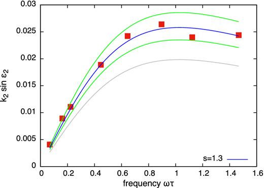
A comparison of the numerically computed quality function, shown as points, to that calculated analytically for a homogeneous Kelvin–Voigt sphere. The analytically derived frequency dependence is given by the grey curve (obtained with equation 25), and when multiplied by s, in blue, with the scaling factor s listed on bottom right. The green curves show the effect of raising and lowering the shear modulus by 10 per cent in the offset analytical calculation. Both the numerical and analytical calculations were carried out for a perturber of mass M* = 100 and initial value of the semimajor axis a0 = 10. We find that the numerically computed quality function has a shape and peak frequency consistent with that obtained analytically, but the amplitude is too high by about 30 per cent. We attribute the scatter of the points off the line to variations in the value of the shear modulus of the random mass-spring network due to non-uniformity in the particle distribution and spring network (see Section 4.2).
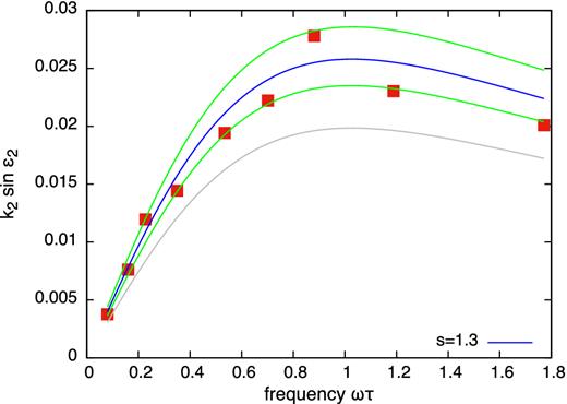
The same as in Fig. 3, except that the perturber's mass is M* = 200, and the initial value of the semimajor axis is a0 = 100.
The numerically generated points in Fig. 3 show that the simulated quality function is proportional to the frequency, at small frequencies, but decays at large frequencies. Predicted analytically for various rheologies (Efroimsky 2012a, 2015; Noyelles et al. 2014), this behaviour has never been reproduced by direct numerical computations. The points used to build this plot were measured from simulations with different spin rates and relaxation times. Nevertheless, they all lie near the same curve, suggesting that the function is primarily dependent on the relaxation time. We thus have numerically confirmed the expected behaviour and sensitivity of the quality function to the frequency and to the viscoelastic time-scale.
With the points obtained through simulations, we plot the quality function predicted analytically using equation (25). We set the shear modulus μ = μI, with the value of μI given by the expression (30). This value is proportional to the Young's modulus listed in Table 1 computed from the spring network. The mass ratio and mean motion are taken from Table 3. The result is the grey line (the lowest one) in Fig. 3. This is the analytically predicted quality function, and we see that its numerically obtained counterpart (given by the red points) is higher. We refer to the ratio of numerically measured quality function to the predicted one as qfratio and from this plot we find qfratio ∼ 1.3.
Fig. 3 demonstrates that the numerically obtained tidal drift rate of the semimajor axis is maximal at a frequency |$\tilde{\chi } \approx 1.0$|, which is consistent with the analytical model. Had the relaxation time-scale (equation 32) been miscomputed in our simulations, the numerically obtained peak would have been displaced away from that predicted analytically. The good match between predicted and numerically measured peak frequency supports our estimate for the shear viscosity (equation 31) and the associated relaxation time (equation 32) for the mass-spring model.
Both the peak magnitude and the peak location of the quality function may shift if higher order terms (with higher values of l) are included into the analytical calculation. As this might explain the difference in height of our numerically computed quality function, compared to that predicted, we tested this possibility by running simulations with a larger value of the semimajor axis. Simulations with a larger initial semimajor axis are also listed in Table 3, and the quality function for these runs is plotted in Fig. 4. We find that the amplitude correction factor required to match the numerical results is the same as for the previous set of simulations – and, again, the frequency does not need to be rescaled. From this, we conclude that higher order terms in the tidal potential do not explain the amplitude discrepancy between our numerical simulations model and our analytical predictions.
Since we are using a random mass-spring model, both the particle distribution and the spring network differ between simulations. We computed the Young's modulus and relaxation time for each run, and these are listed in Table 3. We found small variations in the elastic modulus between different simulations. In Figs 3 and 4, we also show the analytically predicted quality function factored by 1.3 and offset by ± 10 per cent (green curves). Points with higher values of EI, corresponding to harder bodies, systematically lie lower than the appropriate points with lower values of EI corresponding to softer bodies experiencing stronger tidal deformation. The scatter in our points above and below the blue line can be attributed to variations in the particle distribution and in the associated spring network.
4.3 Discrepancy in amplitude of quality function and sensitivity to the number of masses and springs simulated
To see how the discrepancy in amplitude is related to the number of mass nodes and springs, we carried out a second series of simulations each with the same initial spin, estimated elastic modulus, and viscoelastic relaxation time-scale, but having different numbers of node masses and numbers of springs per node. Parameters for these simulations are listed in Table 4. We ran six sets, each of five simulations, all approximately matching the third row in Table 3 with a0 = 10, M*/M = 100, σ0 = −0.4, and Po = 4.377. The five simulations in each set have identical run parameters. The first 10 simulations (columns A, B in Table 4) have about 400 mass nodes, the second 10 (columns C, D) about 800 mass nodes, and the last 10 (columns E, F) about 1600 mass nodes. The first five in each group of 10 have about 10 springs per node (columns A, C, and E) whereas the second five of each group of 10 (columns B, D, and F) have about 20 springs per node. The spring constants, kI, and damping parameters, γI, for each set were chosen so that |$\bar{\chi }\approx 0.225$|, EI ≈ 2.3, and τrelax ≈ 0.155. For each simulation separately we computed ratio qfratio of the numerically measured value of the quality function k2sin ϵ2 to the predicted one computed using the normalized frequency |$\bar{\chi }$| and Young's modulus measured from the nodes and springs in the simulations. We then computed the mean and standard deviation of qfratio for each set of five simulations with identical run parameters and these are listed in the bottom rows of Table 4. The standard deviation in semimajor axis drift rate divided by the mean value of the drift rate is also computed for each set of five simulations and listed in Table 4.
Comparison of simulations with different numbers of node masses and springs per node.
| Set | ||||||
|---|---|---|---|---|---|---|
| A | B | C | D | E | F | |
| 〈NI〉 | 403.8 | 405.8 | 795.2 | 804.2 | 1597.8 | 1596.2 |
| 〈NSI/NI〉 | 10.92 | 18.7 | 11.5 | 20.34 | 12.02 | 21.34 |
| dI | 0.19 | 0.19 | 0.15 | 0.15 | 0.118 | 0.118 |
| ds/dI | 2.3 | 2.8 | 2.2 | 2.8 | 2.3 | 2.8 |
| kI | 0.102 | 0.04 | 0.08 | 0.0301 | 0.062 | 0.023 |
| γI | 12.858 | 5.05 | 20.0 | 7.48 | 31.3 | 11.5 |
| 〈qfratio〉 | 1.48 | 1.39 | 1.41 | 1.36 | 1.40 | 1.38 |
| σ[qfratio] | 0.069 | 0.052 | 0.053 | 0.026 | 0.030 | 0.012 |
| |$\sigma [\dot{a}]/ \langle \dot{a} \rangle$| | 0.061 | 0.064 | 0.055 | 0.024 | 0.026 | 0.0094 |
Notes. With a0 = 10, M* = 100, n = 0.318, σ0 = −0.4, Po = 4.377, |$\bar{\chi }\sim 0.225$|, EI ∼ 2.3, and τrelax ∼ 0.155.
Each column represents a group of five simulations. From each group of five the mean number of nodes and springs per node are listed in the second and third rows. The rows labelled 〈qfratio〉 and σ[qfratio] give the mean and standard deviations, respectively, of the ratio of the numerically measured to analytically predicted quality function. The bottom row gives the ratio of the standard deviation in the semimajor axis drift rate divided by the means. Each of the means and standard deviations are computed from five simulations. The simulations listed here differ from those described by Tables 1 and 3.
In the simulations listed in Tables 1 and 3, the ratio of the number of springs per node is about 11, which is slightly lower than the number recommended by Kot et al. (2015, fig. 5). For this ratio, Kot et al. (2015) found that the spring network behaved 10 per cent weaker6 than what was estimated by equation (29). In Table 4 we can compare the ratio of numerically measured to predicted quality functions for simulations with similar numbers of nodes but differ by the number of springs per node. Comparing columns A to B and C to D and E to F we see that the ratio of numerical measured to predicted quality function is only slightly less (about 2 per cent lower) when the number of springs per node is about 20 rather than 10. We find that for greater than 10 springs per nodes, the ratio of measured to predicted quality function is relatively insensitive to the number of springs per node.
As each simulation generates a new particle distribution and spring network, we can measure effects due to variations in these properties by comparing simulations generated from identical input parameters. Table 4 shows that the standard deviation of the quality function ratio and semimajor axis drift rate decreases with increased particle number and that the scatter in these measured quantities differs by only a few per cent. We conclude that variations in the spring network are unlikely to explain the discrepancy between predicted and numerically measured quality function.
One possible reason for the discrepancy between predicted and measured quality function is that near the body surface the number of springs per particle is lower than the interior, and thus the spring network is anisotropic near the surface. The simulated body is weaker (and floppier) than we estimated by integrating the spring properties over the volume. Because the overall rigidity of the body is weaker, its tidal response would be larger than we predicted analytically. This would be consistent with our greater than unity qfratio. If this were the primary cause of our amplitude discrepancy, then the ratio of numerical computed to analytical predicted quality function should inversely depend on the number of simulated masses. Table 4 shows that this ratio qfratio does decrease as the particle number is increased from 400 to 1600, however, it only decreases by about a per cent between 800 and 1600 particles. Convergence has not been achieved, but the standard deviations in quantities measured from groups of simulations imply that the simulation results are reproducible and that the scatter is smaller than the amplitude discrepancy. If doubling the particle number reduces the quality function ratio by 2 per cent, then to reach a quality function ratio of 1 we would require a million particles in the simulation and we are not yet set up to run simulations this large.
The surface of our body lies within a radius of 1, consequently our simulated body effectively has an outer radius that is smaller than 1. As the semimajor axis drift rate is faster for larger bodies, we would have expected our simulations to exhibit slower rather than faster orbital decay rates (and evident from the factor of R−5 in equation 34). We recall that the analytically predicted quality function depends on the ratio μ/eg (see equations 24 and 25). As the energy density, eg∝R4, for an effective radius less than 1, the energy density is higher than we previously estimated and the ratio μ/eg would be lower than we used. This means we have underestimated the size of the tidal response. This is in the right direction to account for the amplitude discrepancy. However if we take into account both the factor of R5 in equation (34) when computing our numerical quality function and the factor of R4 in equation (25) when computing our analytical quality function, the two corrections more or less cancel each other and we do not resolve the source of discrepancy in quality function amplitude. So we find that we cannot resolve our discrepancy in amplitude by correcting the body radius to an effectively smaller radius.
Equations (29) and (30) characterize static properties of the mass-spring model. However, the analytical theory of evolving tides (including that based on the viscoelastic rheology 15) employs the unrelaxed shear rigidity μ. We have assumed that the two values are equivalent, although this is not perfectly true for real materials. As any rheological parameter, the shear elasticity modulus depends upon frequency. The unrelaxed or frequency-dependent shear modulus in real materials can be lower than the relaxed or static counterpart (e.g. Faul & Jackson 2005). Perhaps this is also true in our simulated material. The numerical tests by Kot et al. (2015) used static forces and so would not have been sensitive to frequency dependence in the shear modulus. Had we employed a smaller value for the shear modulus, this would have increased the values of the theoretically obtained k2 sin ϵ2, and thus would have reduced the offset between our numerical and theoretical values for the quality function.
Each numerical run starts out with a sphere of particles, with springs at their rest lengths. However, after the simulation begins, the body is compressed by self-gravity. The resulting density profile is not perfectly flat, as the centre becomes more compressed than the regions closer to the surface. Furthermore, the initial spin of the body causes its shape to deviate from a sphere. To sample a broad range of frequencies (in units of the relaxation time), and to have a stronger tidal response (i.e. to reduce the simulation time), we use a soft body that is particularly prone to deformation when spun and compressed by self-gravity. Nevertheless our simulated bodies are not strongly deformed and we do not expect body deformation and compression to account for our quality function amplitude discrepancy.
Since our simulated body is composed of randomly distributed point particles, the body is neither exactly spherical nor uniform. Initially, its principal axes of inertia (computed from the moment of inertia tensor) are oriented randomly, and the three moments of inertia are not exactly equal. So, initially, the body's spin angular momentum is not exactly perpendicular to the orbit. In the course of the simulations, we measured the values of the x and y components of the spin angular momentum, finding them to be a few hundredths of the initial z component. This is small enough that the spin about non-polar axes is unlikely to be the cause of our quality function amplitude discrepancy.
To summarize, we have compared simulations with different numbers of mass nodes and springs per node and found that the scatter and sensitivity of the ratio of numerically measured to analytically predicted quality function are only weakly dependent on these quantities. Convergence has not been reached at 1600 simulated particles but the scatter in the simulations is low enough that the variations in the spring network are small enough that we have reproducible numerical measurements and scatter within these measurement are smaller than our measured amplitude discrepancy. We have not identified the source of the 30 per cent discrepancy in the amplitude of our numerically measured quality function, however, we suspect variations in the spring network, floppiness in the outer surface and a possible frequency dependence in the behaviour of the numerically simulated shear modulus.
5 CONCLUSION
In this paper, we have used a self-gravitating damped mass-spring model, within an N-body simulation, to directly model the tidal orbital evolution and rotational spin-up of a viscoelastic body.
We considered a binary composed of an extended body (assumed spherical and homogeneous) and a point-mass companion. Within this setting, we have tested our numerical approach against an analytical calculation for this simple case. The semimajor axis’ tidal evolution rate was calculated by two methods. One was a direct simulation based on simulating the first body with a mass-spring network. Another, analytical, method was based on a pre-conceived viscoelastic model of tidal friction (the Kelvin–Voigt model). The numerically computed tidal evolution of the semimajor axis and the spin rate were a direct outcome of the damped mass-spring model. We compared the results obtained by the two methods, and concluded that a mass-spring network can serve as a faithful model of a tidally deformed viscoelastic celestial body. Specifically, we computed the quality function (the ratio of Love number k2 and the quality factor Q) from the numerically simulated tidal drift of the semimajor axis. The quality function showed a strong frequency dependence that is close to the dependence derived analytically for a Kelvin–Voigt sphere by a method suggested by Efroimsky (2015).
While direct estimates for the global shear and bulk rigidity can be derived from the spring constants and spring lengths, the shear viscosity has not been estimated in the literature. Consequently, we were uncertain of our estimates for the shear viscosity and the associated relaxation time (equation 32). However, a comparison between our computed quality function (specifically the peak frequency) and that predicted analytically for a Kelvin–Voigt solid suggests that our estimates for the numerically simulated shear viscosity and viscoelastic relaxation time were correct.
The magnitude of our numerically predicted quality function is about 30 per cent larger than the one predicted analytically. By comparing simulations performed for two different initial values of the semimajor axis, we concluded that the cause is not the neglect of higher order terms in the quadrupole expansion for the potential. We find the ratio of numerically measured to predicted quality function is only weakly dependent on numbers of mass nodes and springs per node simulated but does slowly decrease with an increase in the numbers of particles simulated. We have not yet identified the cause of the discrepancy. We suspect that the non-uniformity of the spring network at the body surface could have caused a larger than expected tidal response. Alternatively the simulated shear modulus could be frequency dependent and overestimated by its computed static value.
Our study demonstrates that we can directly simulate the tidal evolution of viscoelastic bodies. We currently achieve an accuracy of 30 per cent but with ongoing effort we may improve upon this. It would be difficult to model this process over long (Myr or Byr) time-scales, because the time step is determined by the number of particles within the body and by the spring constants for the links connecting the particles. This requires the time step to be much shorter than the orbital time-scale. Nonetheless, mass-spring models can be used to explore the tidal evolution of inhomogeneous and anisotropic bodies, and to study how their quality functions depend on the rheological properties and internal structure of the body. This fully numerical approach also permits study of tidal phenomena that are not easy to predict analytically – such as capture into (and crossing of) spin–orbit and spin–spin resonances, tidally induced orbital evolution, the distribution of tidal heating, and the effects of non-linear rheological behaviour.
We thank Benoît Noyelles for helpful comments that helped improve the quality of the paper. We also wish to thank Harry Braviner and Moumita Das for helpful discussions, as well as Maciej Kot, Piotr Szymczak, Hanno Rein, and Darin Ragozzine. This work was in part supported by the NASA grant NNX13AI27G.
Darwin's work is presented, in the modern notation, in Ferraz-Mello, Rodríguez & Hussmann (2008).
See Section A5 of Appendix A.
While it is still unknown what rheological models should describe comets and rubble-pile asteroids, both seismic and geodetic data indicate that the Earth's mantle behaves viscoplastically as an Andrade body; see Efroimsky & Lainey (2007), and Efroimsky (2012a,b). At very low frequencies, its behaviour becomes Maxwell (Karato & Spetzler 1990).
Keep in mind that the assumptions of homogeneity and compressibility in Love's theory are mutually contradictive, wherefore this theory can be used only as an approximation (Melchior 1972).
Because of a misprint, fig. 5 in Kot et al. (2015) actually displays (E0 − E)/E0 instead of (E − E0)/E0, with E0 and E being the estimated and measured Young's modulus, respectively (Kot et al., private communication). A smaller average number 〈S〉 of springs per node gives a smaller Young's modulus and a weaker body.
This happens when the spin of a (tidally despun) host star is faster than the orbital period of a close planet orbiting it.
The caveat ‘in time’ is important. Lagging in time does not necessarily imply geometric lagging of the bulge. The lunar orbit being above synchronous, the main (semidiurnal) tide created by the Moon on the Earth always leads, not lags. This, however, gets along well with causality.
With a being the semimajor axis and G the gravity constant, the mean anomaly |${\cal {M}}(t)={\cal {M}}_0(t)+\int ^t_{}\,{\rm d}t\,\sqrt{G(M + M^{\ast })/a^3\,}$| renders the anomalistic mean motion as |$n\equiv {{\dot{\cal {M}}}}={{\dot{\cal {M}}}}_0+\sqrt{G(M + M^{\ast })/a^3\,}$|. In neglect of external perturbations, |${{\dot{\cal {M}}}}_0\approx 0$| and the anomalistic mean motion can be approximated with the Keplerian mean motion: |$n \approx \sqrt{G(M + M^{\ast })/a^3\,}$|.
Sometimes m is also referred to as the azimuthal wavenumber (Ogilvie 2014).
Generally, the two bodies should be treated on equal footing, so this potential should be amended with a similar potential wherewith the extended body is acted upon due to the tides it is exerting on the perturber.
The evolution of the argument of the pericentre ω, the longitude of the node Ω, and the mean motion |${\cal {M}}$| depends overwhelmingly on kl(ωlmpq) sin ϵl(ωlmpq), and also contains terms with kl(ωlmpq) cos ϵl(ωlmpq). The latter terms, though, are very small. It can also be shown that the secular drift of the semimajor axis a, eccentricity e, and inclination i is defined exclusively by the quality functions kl(ωlmpq) sin ϵl(ωlmpq), with no terms containing kl(ωlmpq) cos ϵl(ωlmpq).
REFERENCES
APPENDIX: SEVERAL BASIC FACTS ON BODILY TIDES
Tidal interactions play a key role in evolution of planetary systems and multiple stars. Their signature is observed, e.g. in the synchronized spin of the Moon, the pas de deux of Pluto and Charon, and in the 3:2 spin–orbit resonance of Mercury. Slowly but steadily, tides work to circularize the orbits of planets and moons – or, in some cases, to make orbits eccentric.7 Tidal dissipation warms up close-in moons (like the volcanic Io), close-in planets (like bloated Jupiters), and short-period binary stars (which can experience tidal coalescence).
Referring the reader to Efroimsky (2015), Efroimsky & Makarov (2013), and references therein for a more detailed introduction, here we provide a minimal kit of ideas and formulae needed to talk about bodily tides.
A1 Static tides
The l-degree term |$W_{{\it l}}({\boldsymbol {R}},\,{\boldsymbol {r}})$| of the perturber's potential causes a tidal deformation of the perturbed body, assumed to be linear. Then the resulting lth addition Ul to the perturbed body's potential is also linear in Wl:
|${\boldsymbol {r}}\,^{\prime }$| being an exterior point, and kl being the static Love numbers.
A2 Evolving tides
A3 The secular part of the tidal torque acting on the spin of the extended body
A4 The quality function (‘kvalitet’)
A5 Which terms are leading, and when
This ‘acceding of leadership’ in resonances, along with its physical consequences for binaries, is described in detail in Makarov & Efroimsky (2013) and Makarov, Berghea & Efroimsky (2012). Here we shall only mention two simple examples. Since the Moon is synchronized, the semidiurnal input into the torque acting on its spin is zero. It is then the other components (mainly, the term with {lmpq} = {2201}) that define the tidal response of the Moon and influence its libration in longitude (Makarov et al. 2016). As another example, take Mercury in its 3:2 resonance (Noyelles et al. 2014). For this planet, the {lmpq} = {2201} input into its tidal response is zero, and it is the semidiurnal mode that overwhelmingly defines the tidal response and plays a crucial role in longitudinal libration (Makarov, in preparation).
A6 Tidally generated secular orbital evolution
The tidal potential (equation A8) should be inserted into the Lagrange- or Delaunay-type planetary equations to calculate the secular evolution of the orbit.12 It then turns out after some algebra that the secular orbital evolution is determined mainly by the quality function kl(ωlmpq) sin ϵl(ωlmpq), with the cosine of the lag playing a very marginal role.13
