


Abstract
The Sun's magnetic field exhibits coherence in space and time on much larger scales than the turbulent convection that ultimately powers the dynamo. In the past the α-effect (mean-field) concept has been used to model the solar cycle, but recent work has cast doubt on the validity of the mean-field ansatz under solar conditions. This indicates that one should seek an alternative mechanism for generating large-scale structure. One possibility is the recently proposed ‘shear dynamo’ mechanism where large-scale magnetic fields are generated in the presence of a simple shear. Further investigation of this proposition is required, however, because work has been focused on the linear regime with a uniform shear profile thus far. In this paper we report results of the extension of the original shear dynamo model into the non-linear regime. We find that whilst large-scale structure can initially persist into the saturated regime, in several of our simulations it is destroyed via large increase in kinetic energy. This result casts doubt on the ability of the simple uniform shear dynamo mechanism to act as an alternative to the α-effect in solar conditions.
1 INTRODUCTION
Turbulent motions of plasma within the Sun are believed to be responsible for the generation and sustainment of its magnetic field via dynamo action. It is well understood how small-scale magnetic fields can be induced by the small-scale turbulence (Schekochihin et al. 2004, 2007). A more abstruse phenomenon, however, is the ability for the field to display larger structure on the scale of the Sun itself. Mean field dynamo theory (Moffatt 1978; Rädler & Rheinhardt 2007) which utilises non-zero net helicity via the α-effect (Steenbeck, Krause & Rädler 1966) has long been used to explain the generation of the large-scale fields, although there is recent evidence suggesting that the theory suffers from considerable inaccuracies in the solar context where turbulence is generated by convection (Cattaneo & Hughes 2006; Hughes & Cattaneo 2008). However, if the α-effect is not a plausible model, then how else is large-scale structure to be obtained?
Several authors (Yousef et al. 2008a,b; Heinemann, McWilliams & Schekochihin 2011; McWilliams 2012) have demonstrated an apparently different mechanism. They investigated forced non-helical motion in a long domain in the presence of a uniform shear. They found that magnetic fields with long-range order (and extended lifetimes) can be induced, though the large-scale structures move irregularly and are hard to identify with cyclic behaviour common to the solar field. Their work involved non-helical forcing in order to eliminate the α-effect as an amplification mechanism, as well as a large aspect ratio to allow for large-scale structure to develop whilst conserving computational resolution. A number of theoretical mechanisms have been suggested to explain the ability of shear and non-helical turbulence to generate large-scale fields: an enhanced α via greater correlation of small-scale motions by the shear (Courvoisier, Hughes & Tobias 2009); an interaction with the fluctuating α-effect (Proctor 2007; Richardson & Proctor 2012; Sridhar & Singh 2014); and an enhancement of the shear-current effect (Rogachevskii & Kleeorin 2003; Brandenburg et al. 2008). The enhancement of dynamo action due to shear without an α-effect has also been observed in models incorporating convection (Hughes & Proctor 2009). Recently, Tobias & Cattaneo (2013) showed that it was possible to produce large-scale field with periodic behaviour using a shear dynamo mechanism although this was not a fully 3D simulation.
Our work is an extension of the original ‘shear dynamo’ calculation. The work of Yousef et al. (2008a,b) was performed for the kinematic case only so we have investigated the natural extension of the model by including the Lorentz forces due to the magnetic field. This allows us to determine how the velocity and magnetic fields equilibrate and whether the large-scale structures persist into the non-linear regime.
2 METHODS
To allow for a direct comparison with, and indeed a validation of, the linear regime in the previous work we implement the forcing in an identical fashion to Yousef et al. (2008a). Thus we set the mean forcing power |$\epsilon =\langle \boldsymbol {u}\cdot \boldsymbol {f}\rangle =1$| and inject the energy in a wavenumber shell centred at kf/2π = 3 (i.e. the average forcing scale is lf = 1/3). We broadly use the same parameter values as the previous work so that 0.125 ≤ S ≤ 2 and ν = 10−2 = η giving Rm = Re = urms/kfν ∼ 5 in the linear regime. Simulations with S > 2 cannot be performed within this set-up since in order for the successful separation of scales between the mean and fluctuating parts of the field, the magnitude of the shear must not exceed the turnover rate: urms/lf ∼ 3.
The equations are solved with shear periodic boundary conditions (Umurhan & Regev 2004; Lithwick 2007) using the code snoopy (Lesur & Longaretti 2005, 2007), which utilizes a spectral method. In order to observe the growth and, ultimately, the saturation of the mean magnetic field in this model the size of the domain must be significantly larger than the scale of the turbulent motions. However, this then requires simulations to be run in computationally expensive large boxes for very long durations. Yousef et al. (2008a) alleviated this problem somewhat by using boxes with a large aspect ratio so that one direction of the domain is much longer than the others: Lz ≫ Lx, Ly. Although this reduces computational time drastically we note that several of our simulations (specifically those with very large aspect ratios) had to be run up to 35 times longer than Yousef et al. (2008a) in order to reach the non-linear regime. This shows that several of the simulations in the previous work were extremely far from the saturated regime. It is sufficient to run with 32 points in both the x and y directions, where Lx = 1 = Ly and between 256 and 4096 points in the z direction where 8 ≤ Lz ≤ 128.
3 RESULTS
3.1 Linear regime
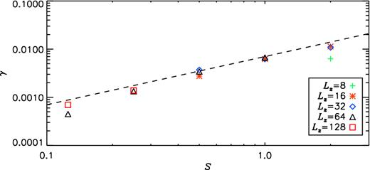
Growth rate of Brms, γ, plotted as a function of the shear rate, S. The dashed line indicates the linear S dependence of γ.
Table displaying the input and output parameters of the simulations performed in this study. Superscripts on lB and By/x indicate that the quantities were calculated for the kinematic (k), the large-scale (l), the small-scale (s) regime, respectively.
| Run | S | Lz | Nz | τf | τs | γ | |$B_{y/x}^{\rm k}$| | |$l_B^{\rm k}$| | |$B_{y/x}^{\rm l}$| | |$l_B^{\rm l}$| | |$B_{y/x}^{\rm s}$| | |$l_B^{\rm s}$| | |
|---|---|---|---|---|---|---|---|---|---|---|---|---|---|
| S0125L64 | 0.125 | 64 | 2048 | 67000 | 35000 | 0.0005 | 10.59 | 12.86 | 219.86 | 57.84 | – | – | |
| S0125L128 | 0.125 | 128 | 4096 | 15000 | – | 0.0007 | 10.52 | 12.82 | – | – | – | – | |
| S025L64 | 0.25 | 64 | 2048 | 40000 | 14000 | 0.0013 | 10.80 | 10.27 | 187.42 | 50.20 | – | – | |
| S025L128 | 0.25 | 128 | 4096 | 25000 | 12000 | 0.0015 | 10.79 | 10.58 | 259.46 | 52.19 | – | – | |
| S05L16 | 0.5 | 16 | 512 | 25000 | 7000 | 0.0028 | 11.28 | 7.44 | 48.03 | 11.94 | – | – | |
| S05L32 | 0.5 | 32 | 1024 | 25000 | 5000 | 0.0037 | 11.41 | 7.91 | 119.35 | 23.35 | – | – | |
| S05L64 | 0.5 | 64 | 2048 | 16000 | 4500 | 0.0036 | 11.29 | 7.92 | 508.56 | 51.48 | – | – | |
| S1L8 | 1 | 8 | 256 | 5000 | – | <0 | – | – | – | – | – | – | |
| S1L16 | 1 | 16 | 512 | 6000 | 3000 | 0.0062 | 11.85 | 5.56 | 68.32 | 10.75 | 4.76 | 1.92 | |
| S1L32 | 1 | 32 | 1024 | 7000 | 2500 | 0.0062 | 12.05 | 5.55 | 285.80 | 23.62 | 4.69 | 1.87 | |
| S1L64 | 1 | 64 | 2048 | 5000 | 2400 | 0.0069 | 11.91 | 5.64 | 164.57 | 21.01 | – | – | |
| S2L8 | 2 | 8 | 256 | 4000 | 2400 | 0.0063 | 12.09 | 3.85 | 62.15 | 6.85 | 4.20 | 1.77 | |
| S2L16 | 2 | 16 | 512 | 3000 | 1500 | 0.0113 | 12.11 | 4.11 | 75.16 | 7.27 | 5.73 | 1.80 | |
| S2L32 | 2 | 32 | 1024 | 3000 | 1300 | 0.0128 | 12.88 | 4.28 | 79.25 | 7.87 | 5.80 | 1.85 |
Structures averaged over the short domains, x and y, are of particular interest because we expect to find large-scale structures appearing in the long domain, z. Such structures do indeed appear, and they are found to wander in space (i.e. z) and time (Fig. 2 for t < 5000, or Fig. 3 for t < 1600) epitomising the non-cyclic behaviour found earlier in this uniform shear case. We find no great qualitative differences between our results and those of Yousef et al. (2008a) indicating that their results are representative of the whole linear regime before the field saturates and Lorentz forces become important. The properties of the linear regime have also recently been confirmed independently by Squire & Bhattacharjee (2015b).
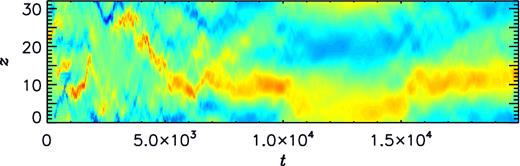
By, averaged over x and y and normalized using Brms, as a function of z and t for simulation S05L32.
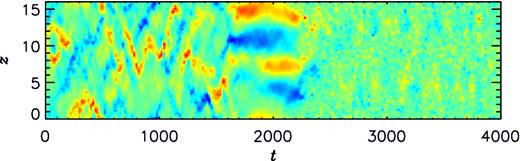
By, averaged over x and y and normalized using Brms, as a function of z and t for simulation S2L16.
3.2 Saturated regime
As the simulations are run further we are able to observe the saturated (i.e. non-linear) regime where the magnetic field equilibrates. In this regime the value of Brms has become large enough for the effect of the Lorentz forces on the velocity field to be important. The time taken to reach the end of the linear regime (τs in Table 1) is, of course, a function of the growth rate and thus varies across the simulations. The quantity τf is the final time that has been reached in each simulation, thus far.
As the magnetic energy ceases to grow, it saturates at an O(1) value, similar to the kinetic energy. At this time we find an immediate growth in the lengthscale of the z-structure of the field in all simulations where it has been possible to reach this time. This is evidenced by the values of |$l_B^{\rm l}$| given in Table 1 as well as graphically in Fig. 4. Fig. 2 (for t > 8000) and Fig. 3 (for 1600 < t < 2200) clearly show that the scale of the field is larger than in the linear regime (cf. with earlier times in the same figures). We find that although the field continues to wander in z-space as time progresses it now does so more slowly. Figs 5 and 6 show the x and y-components of the magnetic field and velocity, respectively, at three different times in the simulation S2L16. Curves are displayed in each plot for specific x and y values as well as averaged over x and y. The averaged z-components are omitted in these plots since the solenoidal conditions stipulate that |$u_z^<=0=B_z^<$|. The z-components at specific x and y values are extremely similar to the x-components and are also omitted in the plots to aid readability. By comparing Fig. 5(a) and (b) we can again see the change in lengthscale of the magnetic field between the regimes.
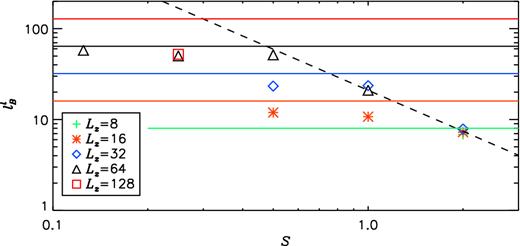
|$l_B^{\rm l}$|, plotted as a function of the shear rate, S, for the large-scale saturated regime. The dashed line indicates a possible S−3/2 dependence of lB. Horizontal lines indicate extent of the box in the z-direction for each Lz.
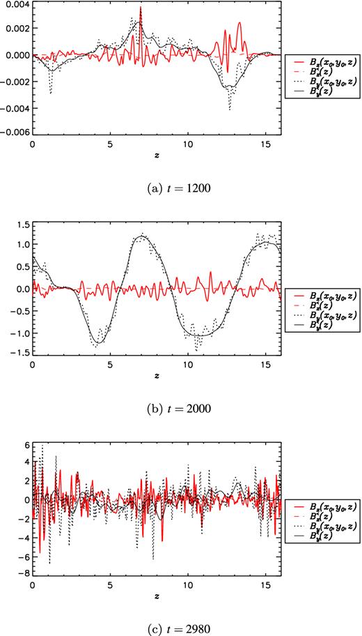
Snapshots of Bx, By (at randomly chosen values of x and y), |$B_x^<$| and |$B_y^<$| as functions of z for simulation S2L16 at three times.
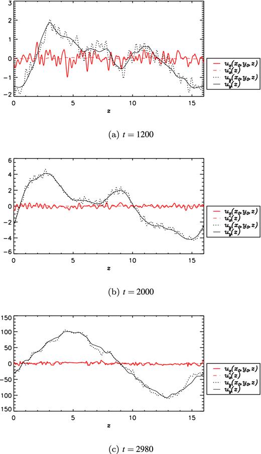
Snapshots of ux, uy (at randomly chosen values of x and y), |$u_x^<$| and |$u_y^<$| as functions of z for simulation S2L16 at three times.
Fig. 4 indicates that an inverse dependence of |$l_B^{\rm l}$| on S (in the form of |$l_B^{\rm l}\sim S^{-3/2}$|, at least for large S) is retained in this regime. However, there is now also some dependence on the box size of the simulation – larger boxes can lead to larger structures. The size of the domain in the z-direction, of course, ultimately limits the size of the structures as |$l_B^{\rm l}$| approaches Lz. The scale of the solution has saturated in the cases S ≥ 1 evidenced by the saturation of |$l_B^{\rm l}$| as the box size is increased. However, for S < 1, larger boxes are required to determine the lengthscale of the field. Unfortunately these computationally expensive simulations are outside the scope of this current work. It therefore seems that, in certain parameter regimes, the aspect ratios chosen by Yousef et al. (2008a) for their original study are not adequate for the non-linear regime. If we assume that the possible lB ∼ S−3/2 dependence shown in Fig. 4 is accurate then we could expect Lz = 64 to be sufficient at S = 0.5 but Lz > 128 is certainly required for S ≤ 0.25.
The transition to a very large-scale field is typical upon entering the non-linear regime across our suite of simulations. The behaviour is also reminiscent of structures in By recently reported by Squire & Bhattacharjee (2015a,b) where it is argued that the coherent large-scale features are driven by small-scale magnetic fluctuations. In their work they either have a small-scale dynamo operating (Squire & Bhattacharjee 2015a) or they force the magnetic field in the same manner as the velocity (Squire & Bhattacharjee 2015b). This is in contrast to our work where Rm is below the threshold value for the onset of a fluctuation (in this regime) and there is no artificial emf imposed – we have time integrated the simulation through the linear regime. Thus the structures we display do not arise as result of small-scale magnetic fluctuations but rather they are a characteristic of the equipartition of the fields in the non-linear regime.
For the majority of simulations the very large-scale field regime persists for the remainder of the duration of time-integration that has (so far) been possible. However, when the shear is large enough we find that a rather different regime can arise typified by a complete destruction of large-scale field (Fig. 3 for t > 2300). Values of |$B^{\rm s}_{y/x}$| and |$l_B^{\rm s}$| are displayed in Table 1 for simulations for which this behaviour has been observed. During the aforementioned large-scale saturated regime the velocity field grows rapidly whilst the magnetic field remains at a saturated value. Most of the kinetic growth is in uy which is organized into the form of a large-scale sinusoidal pattern in z-space (the beginnings of which can be observed in Fig. 6b). This creates a shearing effect in z-space – note that this shear is different from that imposed in the basic state which, by contrast, is linear and dependent on x rather than z. However, there is additional growth in small-scale velocity fluctuations, evidenced by Fig. 7, which has been filtered of the largest lengthscales. The magnitude of the small-scale velocity in the saturated regime (t > 2300) clearly exceeds that of the linear regime (t < 1500). Indeed the rms value of the small-scale velocity is approximately 15 compared with a linear regime value urms ∼ 1 (as found both here and by Yousef et al. 2008a). A larger value of urms consequently leads to a larger Rm and hence the assumption made by Yousef et al. (2008a) that Rm ∼ 5 appears to be invalid in the non-linear regime.

uy, averaged over x and y and bandpass filtered of the three largest modes, as a function of z and t for simulation S2L16.
Once uy becomes large enough, large-scale structure in |$\boldsymbol {B}$| is destroyed enabling a state to develop that is characterized by large-scale structure in |$\boldsymbol {u}$| (Fig. 6c) yet small-scale structure in |$\boldsymbol {B}$| (Fig. 5c). Given that the increase in magnitude of the small-scale velocity is likely to result in Rm exceeding the critical value for the onset of the fluctuation dynamo (Schekochihin et al. 2004, 2007) we postulate that the small-scale nature of the magnetic field in the late saturated regime is the appearance of such a fluctuation dynamo.
4 CONCLUSIONS
In this work we have observed the saturated regime of the shear dynamo problem for a range of parameters similar to those of the original kinematic study (Yousef et al. 2008a). We have found two regimes within the saturated state. The first, which is exhibited in all simulations, is typified by very large-scale structure in By, the magnetic field in the direction of the imposed shear. Structures here are even larger than those found in the kinematic regime (|$l_B^{\rm l}>l_B^{\rm k}$|) although the wandering of field in z-space is reduced. The second regime subsequently appears only in simulations with large imposed shear (S ≥ 1) and displays a drastic reduction in large-scale field. Small-scale field now dominates as the kinetic energy grows rapidly to a new saturated value. While this energy growth is predominantly in the form of a strong z-dependent sinusoidal velocity shear, there is also growth in small-scale velocity structures which consequently increases the value of Rm. It appears likely that the large-scale field previously observed is then overwhelmed by small-scale field generated by a fluctuation dynamo as the value of the magnetic Reynolds number exceeds its required critical value (∼60 for Pm ≥ 1, Schekochihin et al. 2007).
We should note that it is possible that the very large-scale regime found at the onset of saturation may be a intermediate regime at all values of the shear. So far we have only observed a transition to the small-scale regime for S ≥ 1 but that does not preclude the possibility that, with further time-integration, the runs with smaller S could also display such behaviour. Indeed in large boxes with S = 0.5 there is evidence of growth in the kinetic energy similar to that seen at S = 2 which may indicate a progression towards a small-scale regime. Conversely at S = 0.5 with Lz = 16 there is no evidence of kinetic growth despite the total simulation time being over seven times the period of the kinematic regime – such a time period was more than enough to observe the transition in the S = 2 runs. It may be the case that the saturated value of urms in this simulation never becomes large enough for Rm to exceed the critical threshold for the onset of the fluctuation dynamo. However, the value of Rm also depends on, for instance, the magnetic Prandtl number. Hence varying other parameters may allow a fluctuation dynamo to operate at values of S and Lz for which we do not currently see small-scale field in the saturated regime. For S < 0.5 it has not been possible to probe the saturated regime deeply enough to ascertain its behaviour. It is clear from the above discussion that further integration of the simulations, as well as an increase in the aspect ratio of the box, is required to determine the prevalence of the small-scale regime across all values of S, and indeed other parameters. Such simulations are currently too computationally demanding and are left to future work.
Possible inaccuracies in the classical mean-field theory under solar conditions have motivated interest in other dynamo mechanisms such as the shear dynamo. However, if this model with a uniform shear is unable to sustain large-scale field at large, and potentially all, shear rates then its position as a viable alternative to the α-effect may have to be re-examined. There is the option to increase complexity in the current model as a way of potentially negating the undesirable effects leading to the destruction of large-scale field. For instance, Tobias & Cattaneo (2013) have demonstrated in a 2.5D model that an imposed sinusoidal (rather than linear) shear can suppress the generation of small-scale field allowing for the development of large-scale dynamo waves. Such models, however, must be treated with caution until an investigation of the associated non-linear regime is performed, as the results of our current work indicate. An alternative possibility would be to vary the shear along the long domain as a way of adding to the inhomogeneity of the system. Such an extension would be relevant to the Sun where there is known to be a strong differential rotation between the poles and the equator. The ideas discussed here will form the basis of future investigations.
This work was supported by the Science and Technology Facilities Council, grant ST/L000636/1.
REFERENCES
