


Abstract
Cores of relaxed galaxy clusters are often disturbed by AGN. Their Chandra observations revealed a wealth of structures induced by shocks, subsonic gas motions, bubbles of relativistic plasma, etc. In this paper, we determine the nature and energy content of gas fluctuations in the Perseus core by probing statistical properties of emissivity fluctuations imprinted in the soft- and hard-band X-ray images. About 80 per cent of the total variance of perturbations on ∼8–70 kpc scales in the core have an isobaric nature, i.e. are consistent with subsonic displacements of the gas in pressure equilibrium with the ambient medium. The observed variance translates to the ratio of energy in perturbations to thermal energy of ∼13 per cent. In the region dominated by weak ‘ripples’, about half of the total variance is associated with isobaric perturbations on scales of a few tens of kpc. If these isobaric perturbations are induced by buoyantly rising bubbles, then these results suggest that most of the AGN-injected energy should first go into bubbles rather than into shocks. Using simulations of a shock propagating through the Perseus atmosphere, we found that models reproducing the observed features of a central shock have more than 50 per cent of the AGN-injected energy associated with the bubble enthalpy and only about 20 per cent is carried away with the shock. Such energy partition is consistent with the AGN-feedback model, mediated by bubbles of relativistic plasma, and supports the importance of turbulence in the cooling–heating balance.
1 INTRODUCTION
Cores of clusters of galaxies are often perturbed by powerful jets from central supermassive black holes. Interacting with intracluster gas, these jets inflate bubbles of relativistic plasma, which expel the hot gas, producing cavities in the X-ray images of clusters (e.g. Boehringer et al. 1993; Churazov et al. 2000; McNamara et al. 2000; McNamara & Nulsen 2007; Bîrzan et al. 2012; Fabian 2012; Hlavacek-Larrondo et al. 2012). The initial rapid expansion of the bubbles may drive shocks that propagate through intracluster medium (ICM) and heat the gas (e.g. Fabian et al. 2003; Forman et al. 2007; Randall et al. 2015; Reynolds, Balbus & Schekochihin 2015). With time, rapid expansion decelerates and the bubbles continue to grow subsonically until they start rising buoyantly in the cluster atmosphere, uplifting cool gas, exciting gravity waves, and driving turbulence (Churazov et al. 2002; Omma et al. 2004; Zhuravleva et al. 2014a). One of the alternative scenarios is that the bubbles themselves are composed of hot thermal plasma and efficiently mix with the ICM, heating the gas (e.g. Hillel & Soker 2014; Soker, Hillel & Sternberg 2015). However, magnetic fields present in the ICM are likely to stabilize the bubbles and prevent their mixing with the surrounding thermal gas (e.g. Ruszkowski et al. 2007). A combination of turbulent heating and turbulent mixing has also been considered (Kim & Narayan 2003; Dennis & Chandran 2005; Sharma et al. 2009) as well as heating of the gas by cosmic rays through the excitation of Alfvén waves (Pfrommer 2013).
The X-ray-brightest nearby galaxy cluster, the Perseus Cluster, provides a textbook example of radio-mode AGN feedback. Deep Chandra observations of the cluster unveiled distinct perturbations in the hot gas in the innermost ∼100 kpc region, where the physical properties of the gas are governed by the powerful central AGN (Fabian et al. 2011). Namely, we clearly see bubbles of relativistic plasma, shocks, cold filaments and fluctuations induced by motions of the gas. The most recent summary of the observed features in the Perseus core can be found in Fabian et al. (2011). The statistical analysis of the fluctuations was presented in Zhuravleva et al. (2015). In this paper, we attempt to understand how the outflow energy from the central AGN is partitioned between different observed phenomena.
In this paper, we apply a statistical approach to compare the amplitude of emissivity fluctuations in two different energy bands in the Perseus Cluster by measuring the power spectra of fluctuations in both bands and their cross-spectrum. We aim to establish the nature of the observed perturbations in the cluster core, which are induced by the central AGN, and to constrain the energy content associated with each type of perturbation. This work is accompanied by a recent analysis of fluctuations in the Virgo/M87 Cluster (Arévalo et al. 2016) and is the third paper in a series devoted to the statistical analysis of fluctuations in Perseus (see Zhuravleva et al. 2014a, 2015).
2 ISOBARIC, ADIABATIC AND ISOTHERMAL FLUCTUATIONS
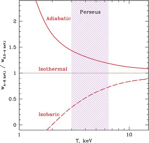
The ratio (equation 6) of emissivity perturbations in two energy bands, 0.5–4 keV and 4–8 keV, as a function of gas temperature, assuming that the perturbations are pure isobaric, isothermal or adiabatic. The purple dotted region shows the range of gas temperatures in the Perseus Cluster. Redshift, galactic H i column density and the abundance of heavy elements Z = 0.5 Z⊙ (relative to the solar abundance of heavy elements; see Anders & Grevesse (1989)) of Perseus are used.
In practice, we are dealing not with the 3D emissivity fluctuation field, but with the projection of this field on to the plane of the sky. However, for a nearly isothermal cluster, the ratio of surface brightness fluctuations in two energy bands is expected to follow equation (6), provided that a single type of perturbation is dominating a region of interest (e.g. Churazov et al., in preparation). The residual images (the initial images divided by the best-fitting spherically symmetric β-models of the surface brightness) of the Perseus Cluster in 0.5–4 keV and 4–8 keV bands, Fig. 2 (see Section 3 for details), show that the amplitude of the spiral-like feature is larger in the soft band than in the hard band, hinting at an isobaric nature of this feature (see Fig. 1). However, in some regions around the central bubbles, the amplitude of perturbations is larger in the hard band, suggesting they have an adiabatic nature. Such visual examination allows us to guess the nature of large-scale and large-amplitude fluctuations. For the less prominent fluctuations that we cannot easily identify in the images, a different, statistical approach is needed.
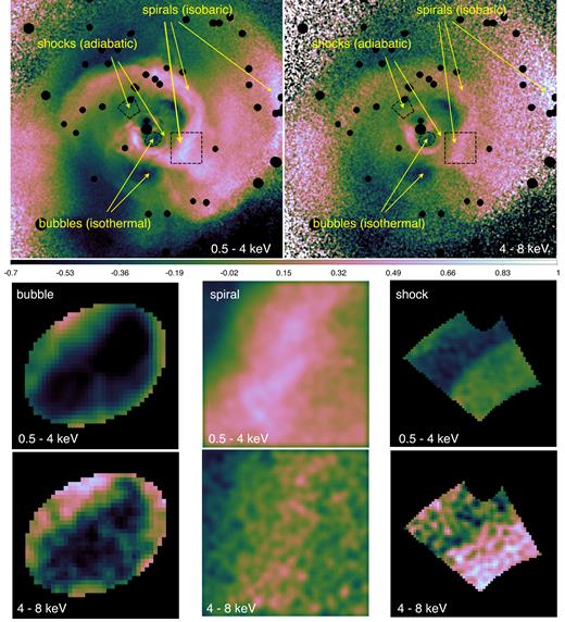
Chandra images of the core (≈200 × 200 kpc, or 9.6 × 9.6 arcmin) of the Perseus Cluster divided by the spherically symmetric β-model in the 0.5–4 keV (top left) and 4–8 keV (top right) bands. Point sources and the central AGN are excised. Arrows point to the prominent features identified in previous studies. Dashed regions indicate selected regions with a shock, a bubble and a spiral. They are enlarged in the middle and bottom panels. The colour scales of the image pairs are the same. For display purposes, all images are lightly smoothed with a 2 arcsec Gaussian.
Since |$\alpha _{\rm isob.}^2+\alpha _{\rm adiab.}^2+\alpha _{\rm isoth.}^2=1$|, the maps of the expected values C and R can be calculated as functions of two parameters αisob. and αadiab., setting |$\alpha _{\rm isoth.}=\sqrt{1-\alpha ^2_{\rm isob.}-\alpha ^2_{\rm adiab.}}$| for any combination of the three types of perturbations. Then, measuring C and R through the observed power and cross-spectra of emissivity fluctuations, equations (9) and (10), and finding these values on C and R maps, the relative contribution of each type of perturbations to the observed total variance of the fluctuations at a given wavenumber k can be obtained.
If the amplitude of fluctuations is large, ∼ few tens per cent, C and R in adiabatic and isobaric cases may differ from those shown in Fig. 1. Our simulations (see Appendix B) show that as long as the amplitude of density fluctuations is ≲ 15 per cent in gas with temperature >3 keV, the ratio is consistent with the values in the limit of small-amplitude perturbations.
3 DATA PROCESSING, IMAGES AND POWER SPECTRA
We use public Chandra data of the Perseus Cluster with total cleaned exposure ≈1.4 Ms. We assume the redshift of the Perseus Cluster z = 0.01755 and the angular diameter distance 71.5 Mpc. 1 arcmin corresponds to a physical scale 20.81 kpc. The total Galactic H i column density is 1.35 × 1021 cm−2 (Dickey & Lockman 1990; Kalberla et al. 2005). The initial data reduction, the details of image processing and the treatment of point sources are described in detail in Zhuravleva et al. (2015, Section 2). Both images, in the 0.5–4 keV and 4–8 keV bands, are treated identically. Masking out point sources and the central AGN, the best-fitting spherically symmetric β-models of surface brightness are obtained. Their parameters are rc = 1.28 (1.48) arcmin and β = 0.53 (0.49) in the soft (hard) band. The images of Perseus divided by the corresponding underlying β-models in both bands are shown in Fig. 2. There are many structures produced by gas perturbations of different nature. The large-scale structures whose nature was identified through ‘X-arithmetic’ analysis (Churazov et al., in preparation) are marked with arrows.
The power and cross-spectra of surface brightness fluctuations in the X-ray images are measured using the modified Δ variance method (Ossenkopf et al. 2008; Arévalo et al. 2012). Subtracting Poisson noise and correcting for the suppression factor associated with 2D → 3D deprojection, which depends only on the global geometry of the cluster, the 3D power spectra of the volume emissivity fluctuations in both bands, Pk, aa and Pk, bb, and the cross-spectrum Pk, ab are calculated. Instead of power spectra, we will show the characteristic amplitude defined as |$A_{k,ab}=\sqrt{4\pi P_{k,ab}k^3}$| (similarly for Ak, aa and Ak, bb) that is a proxy for the rms of emissivity fluctuations δf/f at a given wavenumber k = 1/l. For the data set considered below, the values of Pk, ab are always positive.
Similar analysis was already applied to the analysis of density fluctuations in the AWM7 Cluster (Sanders & Fabian 2012), the Coma Cluster (Churazov et al. 2012), the Perseus Cluster (Zhuravleva et al. 2015), the Virgo Cluster (Arévalo et al. 2016) and the Centaurus Cluster (Walker, Sanders & Fabian 2015). Slightly different approaches have been used to measure pressure fluctuations in the Coma Cluster (Schuecker et al. 2004) and temperature fluctuations in a sample of clusters (Gu et al. 2009). The only difference here from our previous analyses is that here the 2D → 3D deprojection is calculated at each pixel instead of averaged over an area of interest. The underlying β-models are slightly different in two bands since the gas temperature changes with radius. Therefore, we calculate the geometrical correction (the suppression factor) individually for each band. Uncertainties associated with the choice of the underlying β-model and inhomogeneous exposure coverage (see details in Zhuravleva et al. 2015, Section 6) are estimated and taken into account for each fluctuation spectrum presented here.
The analysis of X-ray surface brightness fluctuations directly measures fluctuations of the volume emissivity convolved with Chandra response. In the soft band a, where the temperature dependence of X-ray emissivity is weak, Pk, aa ≈ 4Sk, aa, provided that δn/n ≪ 1 (Churazov et al. 2012). In the hard band, the temperature dependence is significant, and, therefore, the spectrum of the emissivity fluctuations does not correspond to the spectrum of pure density fluctuations.
4 RESULTS
Here we first test our analysis technique in selected regions of the Perseus Cluster that are dominated by prominent, previously identified structures, such as a shock, a bubble or a spiral (Section 4.1). Next, we apply the same analysis to fluctuations in the central (7 × 7 arcmin) region, strongly perturbed by AGN activity, as well as in the region dominated by ripple-like structures (Section 4.2). For each of these cases, we investigate the effects of systematic uncertainties, such as inhomogeneous exposure coverage and the choice of the underlying model (for details, see section 6 of Zhuravleva et al. 2015). We use a uniform weighting scheme when calculating rms of fluctuations present in filtered images, and a spherically symmetric β-model as the underlying model. Our experiments show that various systematic uncertainties do not change our conclusions, although some specific numbers may differ for different weightings or underlying models.
We also tested the cross-spectra technique on simulated X-ray images containing shocks and sound waves (see Appendix C). These tests show that our analysis is able to recover the nature of the dominant type of fluctuation even if the amplitude of the fluctuations is small, ∼ a few per cent.
4.1 Special cases: shock, bubble, spiral
Residual images of three selected regions are shown in Fig. 2. All three regions are within the innermost 30 kpc, where the number of photon counts is large and the gas temperature is ≈3–3.4 keV. For a mean temperature of 3.2 keV, we calculate the C and R maps for all possible combinations of isothermal, adiabatic and isobaric perturbations (Fig. 3, bottom panels). Amplitudes of the volume emissivity fluctuations in the soft and hard bands and cross-amplitude as functions of wavenumber are shown in the top panels of Fig. 3.
![Results of the cross-spectra analysis in regions with the shock (top left), bubble (top middle) and spiral (top right) (see Fig. 2). Top row: amplitude of the volume emissivity fluctuations, in the soft, Ak, aa, (purple) and hard, Ak, bb, (blue) bands and the cross-amplitude, Ak, ab, (black dashed curve); coherence C and ratio R obtained from the observed spectra [equations (9) and (10)]. Blue and purple dotted regions show 1σ statistical and stochastic uncertainties. For clarity, we do not plot the uncertainties on the cross-amplitudes. Our conservative estimates of statistical uncertainties on the measured C and R are shown with the dotted red regions. Bottom row: maps of coherence C (left) and ratio R (right) for a mixture of isobaric, adiabatic and isothermal perturbations in the 3.2 keV gas. Colour bars show the values of C and R [equations (11) and (12)]. The dashed grid shows the values of αi, associated with each type of fluctuation (see Section 2). X-axis: contribution of adiabatic fluctuations αadiab.; Y-axis: contribution of isobaric fluctuations αisob.. The contribution of isothermal fluctuations is $\alpha _{\rm isoth.}=\sqrt{1-\alpha _{\rm adiab.}^2-\alpha _{\rm isob.}^2}$. The maps are schematically divided into three regions where one of the types of perturbations is dominant in terms of total variance. Ellipses show the regions of αisob., αadiab. and αisoth. that correspond to the values of R and C taken from the figures in the top row. Black ellipse: the region with shock, blue ellipse: bubble, white ellipse: spiral. The size of each ellipse reflects the uncertainties associated with Poisson noise, the choice of the underlying model and the choice of the weighting scheme in calculating the power spectra. The locus of C and R is in the adiabatic area if measured in the region with the shock in Perseus, in the isobaric area if obtained from the region with spiral structure and in the isothermal area when the region with the bubble is considered.](https://oup.silverchair-cdn.com/oup/backfile/Content_public/Journal/mnras/458/3/10.1093_mnras_stw520/2/m_stw520fig3.jpeg?Expires=1749849906&Signature=YAB72aSOE2Ezb7O4AvdQQGq6JTJ94UAz4DI9VW1QVpPDzHk7uHZ0hBoJql29Od9TX4H6F98gIOjvZWmNb15xPEjqWndnvaK1TRVOkgdQ-hb-dkTvuEjoGIzQjRv3~k1dtmmlc26qLUsJRXAw2p5QxsQqLAbr4NPD29sHCEhch4vl~qAxrGHqPulqt0lhR9mzka3RN9NL7jfI52TFjwgADnfTJD2ZhrJ8ZyZ4RPbzORJIGQjzSLyHccLGbg33B0~NZLLrSVnBJNpwjPrpDjmuh7XjxNL4BtPzqqhIv7Hnrc~PdyjsWNB-KS~SLA-lHRw8VB3atPqFjnzPRGO~ICrtnA__&Key-Pair-Id=APKAIE5G5CRDK6RD3PGA)
Results of the cross-spectra analysis in regions with the shock (top left), bubble (top middle) and spiral (top right) (see Fig. 2). Top row: amplitude of the volume emissivity fluctuations, in the soft, Ak, aa, (purple) and hard, Ak, bb, (blue) bands and the cross-amplitude, Ak, ab, (black dashed curve); coherence C and ratio R obtained from the observed spectra [equations (9) and (10)]. Blue and purple dotted regions show 1σ statistical and stochastic uncertainties. For clarity, we do not plot the uncertainties on the cross-amplitudes. Our conservative estimates of statistical uncertainties on the measured C and R are shown with the dotted red regions. Bottom row: maps of coherence C (left) and ratio R (right) for a mixture of isobaric, adiabatic and isothermal perturbations in the 3.2 keV gas. Colour bars show the values of C and R [equations (11) and (12)]. The dashed grid shows the values of αi, associated with each type of fluctuation (see Section 2). X-axis: contribution of adiabatic fluctuations αadiab.; Y-axis: contribution of isobaric fluctuations αisob.. The contribution of isothermal fluctuations is |$\alpha _{\rm isoth.}=\sqrt{1-\alpha _{\rm adiab.}^2-\alpha _{\rm isob.}^2}$|. The maps are schematically divided into three regions where one of the types of perturbations is dominant in terms of total variance. Ellipses show the regions of αisob., αadiab. and αisoth. that correspond to the values of R and C taken from the figures in the top row. Black ellipse: the region with shock, blue ellipse: bubble, white ellipse: spiral. The size of each ellipse reflects the uncertainties associated with Poisson noise, the choice of the underlying model and the choice of the weighting scheme in calculating the power spectra. The locus of C and R is in the adiabatic area if measured in the region with the shock in Perseus, in the isobaric area if obtained from the region with spiral structure and in the isothermal area when the region with the bubble is considered.
In the region with a shock (spiral), the amplitude in the hard band is larger (smaller) than in the soft band over a broad range of scales. Emissivity fluctuations have comparable amplitudes in both bands in the ‘bubble’ region.
Fluctuations associated with the shock region have C ≃ 0.90–0.98 and R ≃ 1.3–1.8 on scales between 8 and 20 kpc. On these scales we are effectively comparing the density and temperature of the pre-shock gas to those in the shock-heated gas. The shell has a thickness of ∼8 kpc. The locus of these values on the C and R maps is shown with the black ellipses. They lie within the area dominated by adiabatic perturbations.
Emissivity fluctuations in the region containing the bubble have C ≃ 0.92–0.98 and R ≃ 0.90–1.05 on scales between 4 and 10 kpc. The locus of these values (blue ellipse in Fig. 3) reveals a predominantly isothermal nature of these perturbations with small contamination of adiabatic and isobaric fluctuations, associated with the shock around the bubble and displaced gas, respectively, imprints of which remain in the selected region.
In the region with a spiral structure, we find C ≃ 0.8–0.9 and R ≃ 0.50–0.51 on 10–20 kpc scales. The locus of these values (white ellipse in Fig. 3) confirms the isobaric nature of these fluctuations.
These experiments show that even if the uncertainties are large, the cross-spectra method robustly identifies the dominant type of fluctuations in the X-ray emissivity.
4.2 Central, AGN-dominated region
We now proceed with the analysis of the central r = 3.5 arcmin (≈70 kpc) region, which appears to be disturbed by several types of perturbations and is dominated by a prominent spiral structure and bubbles (Fig. 4). Masking out point sources and the central AGN, we measure the amplitude of the volume emissivity fluctuations in both 0.5–4 keV and 4–8 keV bands, the coherence C and the ratio R shown in the top panels in Fig. 5. Black ellipse on the C − R map in the bottom panel in Fig. 5 shows the locus of the measured values C ≃ 0.80–0.93 and R ≃ 0.50–0.55 on scales ∼8–70 kpc. The approximate centre of the locus gives αadiab. ≃ 0.28, αisob. ≃ 0.88 and the corresponding |$\alpha _{\rm isoth.}=\displaystyle \sqrt{1-\alpha _{\rm adiab.}^2-\alpha _{\rm isob.}^2}\simeq 0.38$|. Therefore, |$\alpha _{\rm isob.}^2\approx 80$| per cent of the total variance can be attributed to isobaric type of fluctuations, less than |$\alpha _{\rm adiab.}^2\approx 8$| per cent of the variance to adiabatic and |$\alpha _{\rm isoth.}^2\approx 14$| per cent to isothermal perturbations. Exclusion of the innermost bubbles and shocks from the central r = 3.5 arcmin region tilts the results towards even larger isobaric fraction.
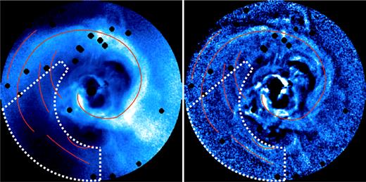
Image of the central r = 3.5 arcmin (≈70 kpc) region of the Perseus Cluster divided by the spherically symmetric β-model of the surface brightness (left) and additionally filtered with the high-pass filter (right); see details in section 6.1 in Zhuravleva et al. (2014a). Point sources and the central AGN are excised. The most prominent ripples are schematically highlighted with red curves. A selected region of the cluster with ripples and without obvious bubbles, central shock, filaments or prominent spiral structure, is shown with dotted boundaries. This region is used in Section 4.2 to test the properties of this subset of ripples.

Results of the cross-spectra analysis in the core of the Perseus Cluster shown in Fig. 4. Left: results from the entire central r ∼ 3.5 arcmin (∼70 kpc) region. Right: results from the selected dotted region (Fig. 4). Top row: amplitude of the volume emissivity fluctuations in the soft and hard bands, cross-amplitudes, measured coherence C and ratio R. Bottom row: the corresponding C and R maps. Notation and colour coding are the same as in Fig. 3. The ellipses show a range of parameters that lead to the observed values of C and R. The sizes of the ellipses reflect statistical and systematic uncertainties. Black ellipse: the entire r = 3.5 arcmin region, white ellipse: the selected dotted region (Fig. 4). The fluctuations in the central region are predominantly isobaric.
The unsharp masking of the Perseus image shows approximate concentric features, so-called ripples, that are narrow in the radial direction and wide in the azimuthal direction (Fabian et al. 2006; Sanders & Fabian 2007). The width of the ripples in the radial direction is roughly 5–15 kpc (see e.g. Fig. 4). Some of the ripples are associated with the brightest and most clearly defined parts of the spiral structure and have an isobaric nature. However, the nature of those ripples that are not associated with the spiral structure is not clear. Two possible scenarios for their origin have been discussed: weak shocks and sound waves propagating through the gas (see e.g. Sanders & Fabian 2007; Graham, Fabian & Sanders 2008a; Fabian et al. 2011, and references therein) or stratified turbulence (Zhuravleva et al. 2014b, 2015). Aiming to understand the physical origin of the ripples, we repeated the cross-spectra analysis of the emissivity fluctuations in the region from which we excised the ripples associated with prominent spiral, bubbles, shocks and filaments (see the dotted region in Fig. 4). The results, shown in Fig. 5 (white ellipse), reveal that the mean value of αadiab. ≃ 0.23, αisob. ≃ 0.7 and αisoth. ≃ 0.67. Therefore, |$\alpha _{\rm isob.}^2\approx 50$| per cent of the total variance is associated with isobaric, |$\alpha _{\rm adiab.}^2\approx 5$| per cent with adiabatic and |$\alpha _{\rm isoth.}^2\approx 45$| per cent with isothermal perturbations on scales ∼12–30 kpc. In other words, the variance presumably induced by the slow motions of the gas in the cluster atmosphere and bubbles constitutes the largest fraction of the total energy in this region on scales larger than 12 kpc. This conclusion does not exclude the presence of ripples associated with shocks and sound waves. However, energetically such perturbations appear to be subdominant. An interesting question would be to understand the nature of fluctuations on smaller scales, less than 12 kpc. Currently, the high level of Poisson noise in the hard band limits our ability to measure the amplitude of emissivity fluctuations on such small scales. For the same reason, it is difficult to perform the analysis for individual ripples. To address these questions, at least twice longer Chandra observations would be needed.
Similar analysis applied to a region outside the inner part of Perseus, the annulus at 3.5–6 arcmin, shows that isobaric fluctuations are again the dominant contributor to the total variance on scales ∼20–50 kpc. In this annulus, the photon statistics in the hard band are too low to constrain the nature of perturbations on smaller scales.
5 DISCUSSION
5.1 Energetics of AGN-driven perturbations and their dissipation time-scale
The measured variance of the volume emissivity fluctuations can be translated into the total energy Epert associated with AGN-induced perturbations in the gas, which we write as Epert = Eb + Esw + Egw, where Eb is the energy in the fluctuations due to bubbles of relativistic plasma (isothermal perturbations), Esw is the energy associated with sound waves and shocks (adiabatic perturbations) and Egw is the energy in fluctuations induced by gravity waves, turbulence or any other slow displacements of the gas (isobaric perturbations). All other contributions are ignored for simplicity. It is convenient to compare these energies to the thermal energy of the gas Eth = PV/(γ − 1) = 3PV/2, where P is its pressure and V is the volume of the region under consideration. Clearly, for each type of perturbation |$E/E_{\rm th}\sim \langle (\delta n/n)^2\rangle \approx \frac{1}{4} \langle (\delta f/f)^2\rangle$| if δf/f is measured in soft (density) band and the perturbation amplitude is small. Let us estimate the proportionality coefficient between E/Eth and δn/n in each case.
5.2 The partition of energy from the central AGN outburst
We showed above that isobaric perturbations are energetically dominant in the inner region of the Perseus Cluster, where gas properties are strongly affected by the central AGN. If these isobaric perturbations are associated with slow gas displacements induced by buoyantly rising and expanding bubbles of relativistic plasma, then the energy from the AGN outburst should be partitioned so that the largest fraction of it goes to the bubbles rather than to shocks or the compressed, shock-heated gas around the bubbles. The partition of the energy depends on the duration of the outburst and on the total outburst energy. Forman et al. (2015) discuss two extreme scenarios: a short-duration outburst, which produces small bubbles surrounded by hot, low-density gas and strong shocks, which carry out most of the AGN energy, and a long-duration outburst, which produces weaker shocks and larger bubbles, which store most of the AGN energy surrounded by the cooler gas. Using 1D numerical simulations of a spherical shock propagating into the gas, Forman et al. (2015) showed that the observational properties of the most prominent shock in the centre of the M87/Virgo Cluster are best described with a long-outburst model with total energy outburst ∼5 × 1057 erg lasting ∼2 Myr. In this model, ≈50 per cent of the injected energy goes into the thermal energy of the bubble and ≈20 per cent is carried away by the shock. Admittedly, the modelling is done under strong assumptions about the source geometry, initial density and temperature profiles, (non-) constant energy injection rate, etc. However, Forman et al. (2015) estimated that the expected uncertainties are only a factor of a few. Below we perform similar analysis for the central shock and bubble in the Perseus Cluster, aiming to understand whether indeed most of the AGN energy is injected into the bubbles. This energy can potentially be later transferred to the gas in the form of isobaric perturbations.
There are several features revealed by deep Chandra observations of the innermost region in Perseus produced by the outburst (Fig. 6a): inner bubbles with size r ≈ 7.5 kpc, distinct shock around one of the bubbles at r ≈ 15 kpc from the bubble centre and a shell of shock-heated gas between the bubble and the front. Modelling of the observed properties of X-ray cavities in the central ∼25 kpc in the Perseus Cluster induced by the relativistic particles of the jet implies a time-averaged nuclear power of the order of 1045 erg s−1(e.g. Heinz et al. 1998; Churazov et al. 2000; Fabian et al. 2000). The deprojection analysis of the gas density shows a density jump at the shock front is 1.25–1.27 (Graham et al. 2008b). Using simulations with a 1D Lagrangian code3 of a spherical shock propagating through the Perseus atmosphere, we will try to reproduce these observed features and check the energy partition that results in these simulations.
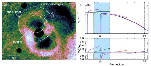
Features produced by the AGN outburst in the innermost region in the Perseus Cluster. (a) the image of the innermost region of the Perseus Cluster (∼60 × 60 kpc) in the 4–8 keV band divided by the best-fitting β-model. Point sources and the central AGN are excised. Dashed circles indicate one of the inner bubbles with the size r ≈ 7.5 kpc and a shock front around it at r ≈ 15 kpc from the bubble centre. (b) Snapshots of simulated density profiles perturbed by a spherical shock, which propagates through the gas in the Perseus Cluster. The shock is driven by an outburst with power 3 × 1044 erg s−1. Black curve shows the initial (unperturbed) density profile, while the colour curves show the profiles at different times after the energy injection starts. The dotted vertical lines indicate the radii of 15 and 60 kpc. The former corresponds to the position of the shock around the inner bubble in Perseus, while the latter shows the approximate location of the distinct ripples. For the shock at ≈15 kpc, the size of the region with the shock-heated gas (shell) is indicated with the shaded blue region. The ratio of the perturbed density to the initial one is shown in the bottom panel.
As initial, unperturbed radial profiles of the gas density and temperature in Perseus, we used the deprojected ones from Zhuravleva et al. (2013). Of course, the initial profiles that might have existed more than 10 Myr ago are quite uncertain. However, if the supermassive black hole is able to maintain a quasi-equilibrium between heating and radiative cooling and the cluster atmosphere has not undergone major changes recently, then we can hope that the present gas distribution is not far from the typical conditions at the time of the outburst. The power of the AGN is chosen so that the size of the density jump at the shock front and the ratio of the shell size to the bubble size rshell/rb approximately match the observed values. Namely, we assume a constant energy injection rate into the bubble LX = 3 × 1044 erg s−1 (roughly consistent with earlier estimates ≈5 × 1044 erg s−1 per bubble; see e.g. Heinz et al. 1998) lasting for 2 × 10⁷ yr. The energy injection is quenched when the bubble expansion becomes subsonic and the bubble size is r ≈ 10 kpc. Subsequently, the shock propagates passively through the cluster atmosphere. As an illustrative example, we show the snapshots of the density radial profiles at different time-steps and the ratio of the perturbed density to the initial one in Fig. 6(b). At Δtinject. = 1.1 × 10⁷ yr after the injection started, the parameters of the simulated features are the closest to the observed ones (see Table 1). Accounting for uncertainties in measurements of the observed features, our conservative estimate of the lower limit on the duration of energy injection is 7 Myr. Note that 5 per cent uncertainties in the density jump and bubble size translate into ≈20 uncertainties in the injected power.
| Observed | Simulated | |
|---|---|---|
| Injected jet power per bubble, LX | ≈5 × 1044 erg s−1(1) | 3 × 1044 erg s−1 |
| Position of the shock front relative to the bubble centre | ≈15 kpc(2) | 15 kpc |
| Amplitude of the density jump at the shock front | 1.25–1.27(3) | 1.25 |
| Ratio of the shell (shock-heated gas) size to the bubble size, rshell/rb | ≈2(2) | 1.9 |
Our simulations provide information about the redistribution of the injected outburst energy at each time-step. When the shock is at 15 kpc from the bubble centre, the total energy released by the AGN is ≈1059 erg. This energy is partitioned so that it gives an excess of thermal energy within the bubble of ≈5 × 1058 erg and in the shock-heated gas of ≈4 × 1058 erg (Fig. 7). After the shock propagation, the total gravitational energy increases by ≈4 × 1057 erg and the total kinetic energy is ≈9.5 × 1057 erg in the entire r = 15 kpc region. This kinetic energy is mostly associated with the kinetic energy of the heated and compressed gas. Note that ≈50 per cent of the outburst energy goes into the excess thermal energy (compared to initial thermal energy) of the bubble and ≈38 per cent, to the excess thermal energy of the compressed and shock-heated gas. The energy in the bubble is larger than in the shell by a factor of 1.3 (the factor is 2.6 if one assumes that the gas inside the bubble is relativistic with the adiabatic index γ = 4/3.). Such energy partition supports the slow-outburst scenario of the energy injection and bubble inflation.4 Finally, the energy carried by the shock is twice larger than the kinetic energy of the heated gas, namely ≈1.9 × 1058 erg, or ≈18 per cent of the injected energy from the AGN (additional energy is associated with the thermal energy of the compressed gas). Note that although the energetics and parameters of the jet, shock and bubble are different from those in the Virgo Cluster (Forman et al. 2015), the way the energy from the central AGN is injected into the gas is the same in both clusters.
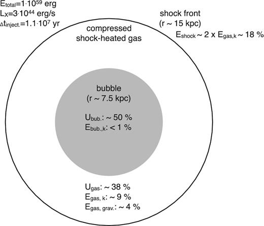
Sketch of the AGN-injected energy partition in the inner 15 kpc in the Perseus Cluster Δtinject. = 1.1 × 10⁷ yr after the injection started. The results are based on 1D simulations of a spherical shock propagating through the cluster atmosphere. The energy is injected at a constant rate LX = 3 × 1044 erg s−1. The total energy released by the AGN up until this moment (when the shock is at 15 kpc from the bubble centre) is Etotal ≈ 1059 erg. The input parameters are shown in the top left corner. About 50 and 38 per cent of the outflow energy is channelled to the excess thermal energies in bubble and in shock-heated gas, respectively. See Section 5.2 for details.
Our modelling implies that indeed the largest fraction of the outburst energy is stored in bubbles and a smaller fraction is transported by a shock. This result relies on the assumption that our 1D approximation and initial conditions provide a reasonable description of the cavity dynamics and the energy partition can be estimated directly from the model. A somewhat different conclusion was reached by Graham et al. (2008a), who used an extrapolation of the pressure profile from the unshocked region to smaller radii to estimate the excess energy. Their approach yields a significantly larger fraction of energy in the shock, suggesting that shock/sound waves dominate transport of energy to the ICM. Our results instead provide support to the bubble-mediated AGN feedback model (Churazov et al. 2000; McNamara et al. 2000; Forman et al. 2007; Nulsen et al. 2007; Bîrzan et al. 2012; Fabian 2012; Hlavacek-Larrondo et al. 2012). Namely, most of the energy is first stored as the enthalpy of the bubbles. As the bubbles rise buoyantly they transfer their energy to the ICM. As we show here, isobaric perturbations dominate the total variance of fluctuations, suggesting that the energy stored within the bubbles could be channelled to the ICM through gravity waves and gas motions induced during the bubble expansion and buoyant rise. The energy of the gas bulk motions eventually dissipates, providing enough heat to offset radiative cooling (Zhuravleva et al. 2014a). The data of future high-energy-resolution missions starting from ASTRO-H will be instrumental in differentiating between the two energy-transporting scenarios mentioned above.
We also looked at the properties of a sound wave produced by the central AGN propagating through the Perseus atmosphere after the energy release is quenching. Simulations show that the amplitude of a passively propagating sound wave leads to density jumps of ≈5 per cent at a distance of 60 kpc, which are consistent with those associated with the ripples in Perseus. At this moment, the energy is partitioned so that the contribution of the kinetic energy of these waves to the total injected energy is small, less than 8 per cent.
We emphasize that these are simple simulations and our analysis neglects many potentially important physical effects, including (but not limited to): heat conduction and viscosity (e.g. Fabian et al. 2005; Ruszkowski & Oh 2011; Gaspari et al. 2014), effects associated with shock propagation through inhomogeneous ICM (e.g. Heinz & Churazov 2005), MHD effects (e.g. Dolag, Bartelmann & Lesch 2002; Mogavero & Schekochihin 2014), the role of cosmic rays (e.g. Pfrommer et al. 2007; Brunetti & Jones 2014). Numerical and theoretical studies showed that these physical processes may strongly affect the gas properties especially on small spatial scales. For instance, strong conduction and/or large viscosity would boost the dissipation of the wave energy as it propagates through the gas, while cosmic rays could change the compressibility of the ICM, tap and redistribute the energy of the shock. However, at present it is difficult to reliably estimate the magnitude of these effects. Current results are valid in the situation when additional physical effects play a subdominant role.
6 CONCLUSIONS
In this work, we investigated the nature of AGN-driven perturbations in the core of the Perseus Cluster and determined the energetically dominant type of perturbations based on the statistical analysis of the X-ray emissivity fluctuations in soft- and hard-band images obtained from deep Chandra observations. We also examined how energy injected by the AGN is partitioned between different feedback channels using 1D hydro-simulations of a shock wave propagating through the Perseus Cluster atmosphere. Our main results are summarized below.
The analysis of cross-spectra is able to recover the dominant type of fluctuations responsible for the fluctuations in the X-ray emissivity even if their amplitude is small, of the order of a few per cent. This is confirmed by various tests that we have carried out using both simulated and observed data.
Most of the emissivity fluctuations induced by the central AGN in the inner ≈140 × 140 kpc region have an isobaric nature (≈80 per cent of the total variance) on scales ∼8–70 kpc, i.e. are consistent with entropy variations that can result from slow displacements of the gas.
In the selected region where there are distinct ripples least contaminated by other structures, about 50 per cent of the total variance of the fluctuations is associated with isobaric perturbations on scales ∼12–30 kpc, supporting the stratified turbulence nature of the ripples (Zhuravleva et al. 2014a). This conclusion does not exclude the presence of ripples associated with shocks or sound waves; however, they are energetically subdominant (≈5 per cent). In order to investigate the nature of individual ripples as well as to probe smaller scales using the cross-spectra analysis, at least twice longer Chandra observations are required. Currently, low photon statistics in the hard band limit the analysis.
Using the fact that the total variance of perturbations is proportional to the energy in perturbations, we estimated that the energy in perturbations is ∼13 per cent of the thermal energy in the inner r = 70 kpc region.
We also estimated the time needed to dissipate the energy from the observed fluctuations into heat to balance radiative cooling. This time is ≈6 × 10⁷–4 × 10⁸ yr.
Simulating the observed properties of the inner shock, bubble and shock-heated gas around the bubble in Perseus, we found that ≈50 per cent of the AGN-injected energy goes into the excess thermal energy of the bubble, ≈40 per cent goes into the compression and heating of the gas between the bubble and the shock front and ≈20 of the injected energy is carried away by the shock. These results are consistent with the bubble-mediated AGN feedback model and support our main results from the cross-spectrum analysis, i.e. the energetically dominant role of slow gas motions that could be induced by the bubbles through the AGN feedback.
Our simulations of the propagating shock show that the contribution of sound waves at distance of 60 kpc from the cluster centre (ripples) to the total excess energy is small, less than 8 per cent. However, a typical amplitude of the simulated ripples of a few per cent is consistent with observations.
The small number of photons, especially in the hard band, limits the analysis presented in this work. The full potential of this method will be unveiled with future X-ray observations that have large effective area (a few tens of times larger than Chandra), such as Athena5 and X-ray Surveyor.6 Having arcsec angular resolution with a few eV spectral resolution, both provided by X-ray Surveyor, will be especially helpful for probing the physics of fluctuations.
Support for this work was provided by the NASA through Chandra award number AR4-15013X issued by the Chandra X-ray Observatory Center, which is operated by the Smithsonian Astrophysical Observatory for and on behalf of the NASA under contract NAS8-03060. IZ thanks A.C. Fabian and J. Sanders for important comments and discussions. EC and AAS are grateful to the Wolfgang Pauli Institute, Vienna, for its hospitality. PA acknowledges support from FONDECYT grant 1140304 and Centro de Astrofisica de Valparaiso. EC and RS are partly supported by grant No. 14-22-00271 from the Russian Scientific Foundation. We are grateful to Hans-Thomas Janka for the provision of a one-dimensional Lagrangian hydrodynamics code, initially used for supernovae explosion calculations.
As the number of photons in the soft band is often larger than in the hard band, the power spectrum of fluctuations in the soft band Pk, aa is used in the denominator in equation (10).
Possibly a continuum of values of ζi in equation (6).
The explicit (first order in space and time) Lagrangian code was provided by H.-T. Janka. The code was initially used for supernova explosion calculations and was adopted to a cluster setup by the authors (see Forman et al. 2007).
Our experiments showed that for a given total injected energy ∼1059 erg, the shortening of the outburst duration leads to a stronger heating of the shock-heated gas. Time-scales shorter than 106 yr correspond to the limiting case of the short-outburst scenario.
REFERENCES
APPENDIX A: CHOICE OF ENERGY BANDS
APPENDIX B: C and R in the case of large-amplitude fluctuations
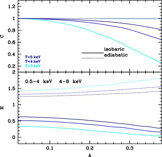
Coherence C and ratio R of emissivity fluctuations in two energy bands, 0.5–4 keV and 4–8 keV, as a function of a parameter A, which characterizes the amplitude of lognormal density fluctuations modelled by equation (B1), for three different gas temperatures in the cases of pure isobaric or adiabatic fluctuations. Note that in the adiabatic case, C does not vary much with the amplitude of fluctuations (as expected) or with gas temperature, in contrast to the isobaric case. For A ≲ 0.15 both C and R only weakly depend on A if the gas is hotter than 3 keV.
APPENDIX C: CROSS-SPECTRA ANALYSIS OF SIMULATED IMAGES WITH SHOCK AND SOUND WAVES
An interesting question is whether the cross-spectra method is able to determine correctly the dominant type of perturbations if their amplitude is small, viz., a few per cent. Using simulated density and temperature radial profiles shown in Fig. 6(b), we obtained the X-ray images in soft and hard bands when the shock was at 15 and 60 kpc (see Section 5.2). Fig. C1 shows the radial profiles of the X-ray surface brightness in both cases. Note a clear discontinuity in the surface brightness when the shock is at 15 kpc and a barely noticeable kink when the shock is at 60 kpc.
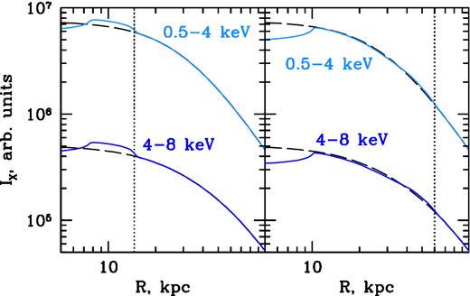
Simulated radial profiles of the X-ray surface brightness IX in the 0.5–4 keV and 4–8 keV bands, calculated from the density and temperature radial profiles modified by the propagating spherical shock in the Perseus Cluster (see Fig. 6b). The unperturbed profiles are shown with black dashed curves. Left: shock at 15 kpc from the bubble centre. Right: shock at 60 kpc.
We fit the profiles with β-models, obtained the residual images of the surface brightness fluctuations and repeated the cross-spectra analysis by measuring the amplitude of the volume emissivity fluctuations in both bands, the cross-amplitude, the correlation C and the ratio R. The results are shown in Fig. C2.
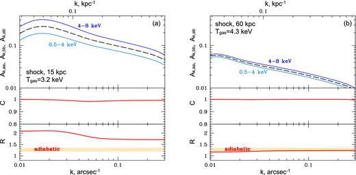
Cross-spectra analysis of simulated images with a shock/sound wave (see Figs 6 b and C1). The amplitude of emissivity fluctuations in both bands and the cross-amplitude are shown in the top panels. Correlation coefficient C and ratio R are shown in the middle and bottom panels, respectively. Expected R (Fig. 1) for pure adiabatic fluctuations is shown with orange regions. (a) Shock at 15 kpc. The analysis is done in the annulus around the shock with the width 0.8 arcmin. (b) Sound wave at 60 kpc. The width of the annulus used for the analysis is 1.6 arcmin. The cross-spectra analysis captures the adiabatic nature of the perturbation in both cases, even if the amplitude of the emissivity fluctuations is small (a few per cent).
First, we analysed fluctuations in the annulus with a width of 0.8 arcmin around the shock at 15 kpc. The annulus width roughly matches the size of the region with the shock in the observed images that we considered earlier (see Fig. 2). The amplitude of emissivity fluctuations is ≈26 per cent and ≈14 per cent (Fig. C2) at ∼10 kpc scales in the soft and hard bands, respectively. These values are close to those obtained from observations in the extraction region of similar size. If wider annulus is used, the amplitudes derived from simulations go down compared to observations because in the latter, other perturbations besides the shock front contribute to the surface-brightness fluctuations. In contrast, the measured coherence and ratio are very stable. The measured coherence C ≈ 1 (Fig. C2) confirms the presence of only one type of perturbations. The ratio R ∼ 1.9 at 10 kpc scale is slightly higher than the predicted value 1.4–1.6 (Fig. 1). This deviation can be due to the temperature variations in the chosen region and the relatively large amplitude of emissivity fluctuations. Also the choice of the underlying model may affect the results, especially on large scales. Nevertheless, we can confidently exclude perturbations of an isothermal (R = 1) or isobaric (R < 0.4) nature.
For the sound wave at 60 kpc, we consider a broader annulus of width 1.6 arcmin, which roughly matches the size of the dotted region in Fig. 4. The measured amplitudes of the emissivity fluctuations are ∼4.5 and ∼6 per cent on scales of ∼20 kpc in the soft and hard bands, respectively (Fig. C2), which are lower than the observed value, ∼12 per cent, in Perseus (Fig. 5). The measured amplitude strongly depends on the size of the region analysed. However, both C ≈ 1 and R ≈ 1.2 robustly confirm the adiabatic nature of the perturbations. This test shows that the cross-spectra analysis is powerful enough to determine the dominant type of perturbations even if the amplitude of emissivity fluctuations is only a few Per cent.
