


Abstract
We present the first reported case of the simultaneous metallicity determination of a gamma-ray burst (GRB) host galaxy, from both afterglow absorption lines as well as strong emission-line diagnostics. Using spectroscopic and imaging observations of the afterglow and host of the long-duration Swift GRB 121024A at z = 2.30, we give one of the most complete views of a GRB host/environment to date. We observe a strong damped Lyα absorber (DLA) with a hydrogen column density of log |$N({\rm H\,{\small I}})\,=\,21.88\pm 0.10$|, H2 absorption in the Lyman–Werner bands (molecular fraction of log(f) ≈−1.4; fourth solid detection of molecular hydrogen in a GRB-DLA), the nebular emission lines Hα, Hβ, [O ii], [O iii] and [N ii], as well as metal absorption lines. We find a GRB host galaxy that is highly star forming (SFR ∼ 40 M⊙ yr−1), with a dust-corrected metallicity along the line of sight of [Zn/H]corr = −0.6 ± 0.2 ([O/H] ∼ −0.3 from emission lines), and a depletion factor [Zn/Fe] = 0.85 ± 0.04. The molecular gas is separated by 400 km s−1 (and 1–3 kpc) from the gas that is photoexcited by the GRB. This implies a fairly massive host, in agreement with the derived stellar mass of log(M★/M⊙) = |$9.9^{+0.2}_{-0.3}$|. We dissect the host galaxy by characterizing its molecular component, the excited gas, and the line-emitting star-forming regions. The extinction curve for the line of sight is found to be unusually flat (RV ∼ 15). We discuss the possibility of an anomalous grain size distributions. We furthermore discuss the different metallicity determinations from both absorption and emission lines, which gives consistent results for the line of sight to GRB 121024A.
1 INTRODUCTION
The study of gamma-ray burst (GRB) afterglows has proven to be a powerful tool for detailed studies of the interstellar medium (ISM) of star-forming galaxies, out to high redshifts (e.g. Vreeswijk et al. 2004; Prochaska et al. 2007; Ledoux et al. 2009; Sparre et al. 2014). With quickly fading emission spanning the entire electromagnetic spectrum, GRB afterglows offer a unique opportunity to probe the surrounding environment. The intrinsic spectrum of the afterglow is well fitted with simple power-law segments, so the imprints of the intergalactic medium (IGM) as well as the ISM surrounding the burst are relatively easy to distinguish from the afterglow in the observed spectrum. Moreover, with absorption and emission-line analysis it is possible to determine parameters such as H i column density, metallicity, dust depletion, star formation rate (SFR) and kinematics of the GRB host galaxy.
Metallicity is a fundamental parameter for characterizing a galaxy and it holds important information about its history. Metallicity might also play a crucial role in the GRB production mechanism. For GRB hosts, the metallicity is measured either from hydrogen and metal absorption lines, or by using diagnostics based on the fluxes of strong nebular emission lines, calibrated in the local Universe. Different calibrations are in use leading to some discrepancy (e.g. Kudritzki et al. 2012), and the different diagnostics have their strengths and weaknesses (e.g. less sensitive to reddening, multiple solutions, or more sensitive at high metallicities). The absorption lines probe the ISM along the line of sight, while the nebular line diagnostics determine the integrated metallicity of the H ii regions of the host. For GRB damped Lyα absorbers (GRB-DLAs, N(H i)>2 × 1020 cm−2; Wolfe, Gawiser & Prochaska 2005), a direct comparison of metallicity from the two methods is interesting because it can either provide a test of the strong-line methods or alternatively allow a measurement of a possible offset in abundances in H ii regions and in the ISM. So far, this comparison has only been carried out for a few galaxy counterparts of DLAs found in the line of sight of background QSOs (QSO-DLAs, e.g. Bowen et al. 2005; Noterdaeme et al. 2012; Péroux et al. 2012; Fynbo et al. 2013; Jorgenson & Wolfe 2014). To our knowledge, a comparison for GRB-DLAs has not been reported before. For both emission and absorption measurements to be feasible with current instrumentation, the observed host needs to be highly star forming, to have strong nebular lines, and at the same time be at a redshift high enough for the Lyα transition to be observed (at redshifts higher than z ≈ 1.5 the Lyα absorption line is redshifted into the atmospheric transmission window). GRB 121024A is a z = 2.30 burst hosted by a highly star-forming galaxy. We measure abundances of the GRB host galaxy in absorption and compare them with the metallicity determined by strong-line diagnostics using observed nebular lines from [O ii], [O iii], [N ii] and the Balmer emission lines.
Apart from the absorption features from metal lines, we also detect the Lyman–Werner bands of molecular hydrogen. Molecular hydrogen is hard to detect in absorption, because it requires high S/N and mid-high resolution. As long duration GRBs (tobs > 2 s) are thought to be associated with the death of massive stars (e.g. Hjorth et al. 2003; Stanek et al. 2003; Sparre et al. 2011; Cano 2013; Schulze et al. 2014), they are expected to be found near regions of active star formation, and hence molecular clouds. In spite of this, there are very few detections of molecular absorption towards GRBs (see e. g Tumlinson et al. 2007). Ledoux et al. (2009) found that this is likely due to the low metallicities found in the systems observed with high-resolution spectrographs (R = λ/Δλ ≳ 40 000). Typically, mid/high-resolution spectroscopy at a sufficient S/N is only possible for the brighter sources. As is the case for QSO-DLAs, lines of sight with H2 detections will preferentially be metal-rich and dusty. The observed spectra are therefore UV-faint and difficult to observe (GRB 080607 is a striking exception, where observations were possible thanks to its extraordinarily intrinsic luminosity and rapid spectroscopy; see Prochaska et al. 2009). Now with X-shooter (Vernet et al. 2011) on the Very Large Telescope (VLT), we are starting to secure spectra with sufficient resolution to detect H2 for fainter systems resulting in additional detections (Krühler et al. 2013; D'Elia et al. 2014).
Throughout this paper, we adopt a flat Λ cold dark matter cosmology with H0 = 71 km s−1 and ΩM = 0.27, and report 1σ errors (3σ limits), unless otherwise indicated. Reference solar abundances are taken from Asplund et al. (2009), where either photospheric or meteoritic values (or their average) are chosen according to the recommendations of Lodders, Palme & Gail (2009). Column densities are in cm−2. In Section 2, we describe the data and data reduction used in this paper, in Section 3 we present the data analysis and results, which are then discussed in Section 4.
2 OBSERVATIONS AND DATA REDUCTION
On 2012 October 24 at 02:56:12 ut the Burst Alert Telescope (BAT; Barthelmy et al. 2005) onboard the Swift satellite (Gehrels et al. 2004) triggered on GRB 121024A. The X-Ray Telescope (XRT) started observing the field at 02:57:45 ut, 93 s after the BAT trigger. About 1 min after the trigger, Skynet observed the field with the Panchromatic Robotic Optical Monitoring and Polarimetry Telescopes (PROMPT) telescopes located at CTIO in Chile and the 16 arcsec Dolomites Astronomical Observatory telescope (DAO) in Italy (Reichart et al. 2005) in filters g′, r′, i′, z′ and BRi. Approximately 1.8 h later, spectroscopic afterglow measurements in the wavelength range of 3000–25 000 Å were acquired (at 04:45 ut), using the cross-dispersed, echelle spectrograph X-shooter (Vernet et al. 2011) mounted at ESO's VLT. Then at 05:53 ut, 3 h after the burst, the Gamma-Ray burst Optical/NIR Detector (GROND; Greiner et al. 2007, 2008) mounted on the 2.2 m MPG/ESO telescope at La Silla Observatory (Chile), performed follow-up optical/NIR photometry simultaneously in g′, r′, i′, z′ and JHK. About 1 yr later (2013 November 07), VLT/HAWK-I imaging of the host was acquired in the J (07:02:13 ut) and K (06:06:47 ut) band. To supplement these, B-, R- and i-band imaging was obtained at the Nordic Optical Telescope (NOT) at 2014 January 06 (i) and February 10 (R) and 19 (B). Gran Telescopio Canarias (GTC) observations in the g and z band were optioned on 2014 February 28. For an overview see Tables 1–3. Linear and circular polarization measurements for the optical afterglow of GRB 121024A have been reported in Wiersema et al. (2014).
X-shooter observations.
| tobs (ut)a | tGRB (min)b | texp. (s) | Mean Airmass | Seeing |
|---|---|---|---|---|
| 04:47:01 | 116 | 600 | 1.23 | 0.6–0.7 arcsec |
| 04:58:35 | 127 | 600 | 1.19 | 0.6–0.7 arcsec |
| 05:10:12 | 139 | 600 | 1.16 | 0.6–0.7 arcsec |
| 05:21:46 | 151 | 600 | 1.13 | 0.6–0.7 arcsec |
| tobs (ut)a | tGRB (min)b | texp. (s) | Mean Airmass | Seeing |
|---|---|---|---|---|
| 04:47:01 | 116 | 600 | 1.23 | 0.6–0.7 arcsec |
| 04:58:35 | 127 | 600 | 1.19 | 0.6–0.7 arcsec |
| 05:10:12 | 139 | 600 | 1.16 | 0.6–0.7 arcsec |
| 05:21:46 | 151 | 600 | 1.13 | 0.6–0.7 arcsec |
Notes.aStart time of observation on 2012 October 24.
bMid-exposure time in seconds since GRB trigger.
X-shooter resolution.
| Arm | Slit | R = λ/Δλ |
|---|---|---|
| NIR | 0.9 arcsec | 6800 |
| VIS | 0.9 arcsec | 13 000 |
| UVB | 1.0 arcsec | 7100 |
| Arm | Slit | R = λ/Δλ |
|---|---|---|
| NIR | 0.9 arcsec | 6800 |
| VIS | 0.9 arcsec | 13 000 |
| UVB | 1.0 arcsec | 7100 |
X-shooter resolution.
| Arm | Slit | R = λ/Δλ |
|---|---|---|
| NIR | 0.9 arcsec | 6800 |
| VIS | 0.9 arcsec | 13 000 |
| UVB | 1.0 arcsec | 7100 |
| Arm | Slit | R = λ/Δλ |
|---|---|---|
| NIR | 0.9 arcsec | 6800 |
| VIS | 0.9 arcsec | 13 000 |
| UVB | 1.0 arcsec | 7100 |
Photometric observations.
| Instrument | Timea | Filter | Exp. time (s) | Seeing | Mag (Vega) |
|---|---|---|---|---|---|
| MPG/GROND | 3.0 h | g′ | 284 | 1.55 arcsec | 20.79 ± 0.07 |
| MPG/GROND | 3.0 h | r′ | 284 | 1.40 arcsec | 19.53 ± 0.05 |
| MPG/GROND | 3.0 h | i′ | 284 | 1.26 arcsec | 19.05 ± 0.07 |
| MPG/GROND | 3.0 h | z′ | 284 | 1.39 arcsec | 18.66 ± 0.08 |
| MPG/GROND | 3.0 h | J | 480 | 1.36 arcsec | 17.84 ± 0.09 |
| MPG/GROND | 3.0 h | H | 480 | 1.29 arcsec | 16.98 ± 0.10 |
| MPG/GROND | 3.0 h | Ks | 480 | 1.21 arcsec | 16.07 ± 0.11 |
| VLT/HAWK-I | 355.2 d | J | 240 × 10 | 0.6 arcsec | 22.4 ± 0.1 |
| VLT/HAWK-I | 355.1 d | K | 240 × 10 | 0.5 arcsec | 20.8 ± 0.2 |
| NOT/ALFOSC | 483.9 d | B | 5 × 480 | 1.3 arcsec | 24.2 ± 0.2 |
| NOT/ALFOSC | 475.0 d | R | 9 × 265 | 1.1 arcsec | 23.8 ± 0.3 |
| NOT/ALFOSC | 440.0 d | i | 9 × 330 | 0.9 arcsec | 23.8 ± 0.3 |
| GTC/OSIRIS | 491.3 d | g′ | 3 × 250 | 1.6 arcsec | 24.9 ± 0.1 |
| GTC/OSIRIS | 491.3 d | z′ | 10 × 75 | 1.4 arcsec | 23.2 ± 0.3 |
Notes.aTime since the GRB trigger (observer's time frame).
For the afterglow measurements time is given in hours, while for the host galaxy, it is shown in days.
2.1 X-shooter NIR / Optical / UV spectroscopy
The X-shooter observation consists of four nodded exposures with exposure times of 600 s each, taken simultaneously by the ultraviolet/blue (UVB), visible (VIS) and near-infrared (NIR) arms. The average airmass was 1.18 with a median seeing of ∼0.7 arcsec. The spectroscopy was performed with slit-widths of 1.0, 0.9 and 0.9 arcsec in the UVB, VIS and NIR arms, respectively. The resolving power R = λ/Δλ is determined from telluric lines to be R = 13 000 for the VIS arm. This is better than the nominal value due to the very good seeing. Following Fynbo et al. (2011), we then infer R = 7100 and 6800 for the UVB and NIR arms, see Table 2 for an overview.
X-shooter data were reduced with the ESO/X-shooter pipeline version 2.2.0 (Goldoni et al. 2006), rectifying the data on an output grid with a dispersion of 0.15 Å pixel−1 in the UVB, 0.13 Å pixel−1 in the VIS and 0.5 Å pixel−1 in the NIR arm. The wavelength solution was obtained against arc-lamp frames in each arm. Flux-calibration was performed against the spectrophotometric standard GD71 observed during the same night. We further correct the flux-calibrated spectra for slit-losses by integrating over filter curves from GROND photometry shifted to X-shooter observation times (assuming a slope of α = 0.8). For the UVB arm, only the g′ band photometry is available, which covers the DLA (see Section 3.1), making this calibration less secure. Wavelengths are plotted in vacuum and corrected for heliocentric motion.
2.2 NOT, GTC and VLT/HAWK-I imaging
To derive physical parameters of the host of GRB 121024A via stellar population synthesis modelling, we obtained late-time photometry from VLT / HAWK-I, NOT and GTC. Exposure times and seeing can be found in Table 3.
J- and K-band images were observed with HAWK-I on the Yepun (VLT-UT4) telescope at the ESO Paranal Observatory in Chile. HAWK-I is a near-infrared imager with a pixel scale of 0.106 arcsec pix−1 and a total field of view of 7.5 arcmin × 7.5 arcmin. B, R and i images were obtained with the ALFOSC optical camera on the NOT. The photometric calibration was carried out by observing the standard star GD71 at a similar airmass to the GRB field. g′- and z′-band host galaxy images were taken with the 10.4 m GTC. The images were acquired with the OSIRIS instrument which provides an unvignetted field of view of 7.8 arcmin × 7.8 arcmin and a pixel scale of 0.25 arcsec pix−1 (Cepa et al. 2000). Images were taken following a dithering pattern. The z′-band images were defringed by subtracting an interference pattern which was constructed based on the dithered individual frames. The photometric calibration was carried out by observing the standard star SA95-193 (Smith et al. 2002). NOT and GTC are located at the observatory of Roque de los Muchachos, La Palma, Spain.
All images were dark-subtracted and flat-fielded using iraf standard routines.
2.3 GROND and Skynet photometry
GROND data was reduced using standard iraf tasks (Tody 1997; Krühler et al. 2008). The afterglow image was fitted using a general point spread function (PSF) model obtained from bright stars in the field. The optical images in g′, r′, i′, z′ were calibrated against standard stars in the SDSS catalogue, with an accuracy of ±0.03 mag. The NIR magnitudes were calibrated using stars of the 2MASS catalogue, with an accuracy of ±0.05 mag. Skynet obtained images of the field of GRB 121024A on 2012 October 24–25 with four 16 arcsec telescopes of the PROMPT array at CTIO, Chile, and the 16 arcsec DAO in Italy. Exposures ranging from 5 to 160 s were obtained in the BVRI (PROMPT) and g′, r′, i′ (DAO) bands, starting at 02:57:07 ut (t = 55 s since the GRB trigger) and continuing until t = 7.3 h on the first night, and continuing from t = 20.7–25.5 h on the second night. Bias subtraction and flat-fielding were performed via Skynet's automated pipeline. Post-processing occurred in Skynet's guided analysis pipeline, using both custom and iraf-derived algorithms. Differential aperture photometry was performed on single and stacked images, with effective exposure times of 5 s–20 min on the first night, and up to ∼4 h on the second night. Photometry was calibrated to the catalogued B, V, g′, r′, i′ magnitudes of five APASS DR7 stars in the field, with g′, r′, i′ magnitudes transformed to RI using transformations obtained from prior observations of Landoldt stars (Henden et al., in preparation). The Skynet magnitudes can be seen in Appendix A.
3 ANALYSIS AND RESULTS
3.1 Absorption lines
The most prominent absorption feature is the Lyα line. We plot the spectral region in Fig. 1. Overplotted is a Voigt-profile fit to the strong Lyα absorption line yielding log |$N({\rm H\,{\small I}})=21.88\pm 0.10$|. The error takes into account the noise in the spectrum, the error on the continuum placement and background subtraction at the core of the saturated lines. Table 4 shows the metal absorption lines identified in the spectrum. To determine the ionic column densities of the metals, we model the identified absorption lines with a number of Voigt-profile components, as follows. We use the Voigt-profile fitting software vpfit1 version 9.5 to model the absorption lines. We first normalize the spectrum around each line, fitting featureless regions with zero- or first-order polynomials. To remove the contribution of atmospheric absorption lines from our Voigt-profile fit, we compare the observed spectra to a synthetic telluric spectrum. This telluric spectrum was created following Smette, Sana & Horst (2010) as described by De Cia et al. (2012) and assuming a precipitable water-vapour column of 2.5 mm. We systematically reject from the fit the spectral regions affected by telluric features at a level of >1 per cent.2 None of the absorption lines that we include are severely affected by telluric lines. The resulting column densities are listed in Tables 4 and 5 for lines arising from ground-state and excited levels, respectively. We report formal 1σ errors from the Voigt-profile fitting. We note that these do not include the uncertainty on the continuum normalization, which can be dominant for weak lines (see e.g. De Cia et al. 2012). We hence adopt a minimum error of 0.05 dex to account for this uncertainty. The error on the redshifts of each component is 0.0001. The Voigt-profile fits to the metal lines are shown in Figs 2 and 3.
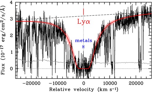
The UVB spectrum centred on the DLA line at the GRB host galaxy redshift. For clarity purposes, the spectrum has been smoothed with a median filter with a sliding window width of 3 pixels. A neutral hydrogen column density fit (log |$N({\rm H\,\,\small {I}})\,=\,21.88\pm 0.10$|) to the damped Lyα line is shown with a solid line (red), while the 1σ errors are shown with the shaded area (also red). In blue is shown the velocity range of the metal absorption lines. The dashed line shows the continuum placement, while the grey line near the bottom shows the error spectrum.
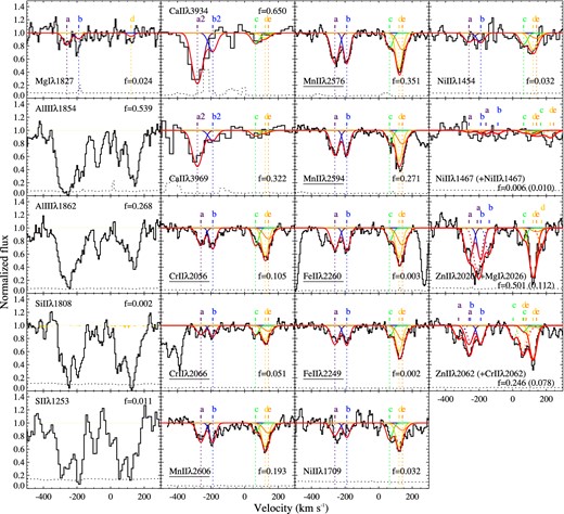
Velocity profiles of the metal resonance lines. Black lines show the normalized spectrum, with the associated error indicated by the dashed line at the bottom. The Voigt-profile fit to the lines is marked by the red line, while the single components of the fit are displayed in several colours (vertical dotted lines mark the centre of each component). The decomposition of the line-profile was derived by modelling only the underlined transitions. The oscillator strength ‘f’, is labelled in each panel. Saturated lines have not been fitted with a Voigt-profile, so for these we show only the spectrum.
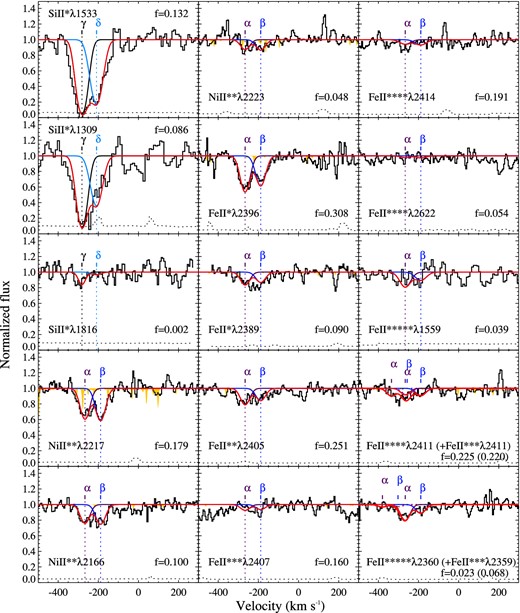
The same as Fig. 2, but for fine-structure lines. Telluric features are highlighted in yellow.
Ionic column densities of the individual components of the line profile. The transitions used to derive column densities are reported in the second column. Transitions marked in bold are those unblended and unsaturated lines that we use to determine the line-profile decomposition. The results for the ground state and excited levels are listed in the top and bottom part of the table, respectively. Velocities given are with respect to the [O iii] λ5007 line (z = 2.3015). (b)/(s) indicate that the line is blended/saturated. The error on the redshifts of each component is 0.0001.
| Component | Transition | a | b | c | d | e |
|---|---|---|---|---|---|---|
| z | – | 2.2981 | 2.2989 | 2.3017 | 2.3023 | 2.3026 |
| b (km s−1) | – | 26 | 21 | 20 | 22 | 35 |
| v (km s−1) | – | −264 | −191 | 64 | 118 | 145 |
| log(N) | ||||||
| Mg i | λ1827, λ2026(b) | 13.97 ± 0.05 | 13.57 ± 0.05 | <13.4 | 13.57 ± 0.07 | <13.4 |
| Al iii | λ1854(s), λ1862(s) | – | – | – | – | – |
| Si ii | λ1808(s) | – | – | – | – | – |
| S ii | λ1253(s) | – | – | – | – | – |
| Ca ii | λ3934, λ3969 | 13.25 ± 0.16a | 12.50 ± 0.16b | 12.20 ± 0.16 | 11.90 ± 0.16 | 11.20 ± 0.16 |
| Cr ii | |$\boldsymbol{\lambda }$|2056, λ2062(b), |$\boldsymbol{\lambda }$|2066 | 13.47 ± 0.05 | 13.48 ± 0.05 | 13.39 ± 0.05 | 13.67 ± 0.05 | 13.34 ± 0.09 |
| Mn ii | |$\boldsymbol{\lambda }$|2576, |$\boldsymbol{\lambda }$|2594, |$\boldsymbol{\lambda }$|2606 | 13.15 ± 0.05 | 13.07 ± 0.05 | 12.71 ± 0.05 | 13.21 ± 0.05 | 12.93 ± 0.05 |
| Fe ii | λ1611, |$\boldsymbol{\lambda }$|2260, |$\boldsymbol{\lambda }$|2249 | 15.15 ± 0.05 | 15.09 ± 0.05 | 14.81 ± 0.05 | 15.27 ± 0.05 | 15.12 ± 0.05 |
| Ni ii | λ1345, λ1454, λ1467.3, λ1467.8, λ1709 | 13.91 ± 0.10 | 13.88 ± 0.10 | 13.95 ± 0.09 | 14.17 ± 0.10 | 13.73 ± 0.29 |
| Zn ii | λ2026(b), λ2062(b) | 13.14 ± 0.05 | 13.05 ± 0.05 | 12.50 ± 0.08 | 13.40 ± 0.05 | 12.19 ± 0.40 |
| Component | – | α | β | – | – | – |
| z | – | 2.2981 | 2.2989 | – | – | – |
| b (km s−1) | – | 28 | 30 | – | – | – |
| v (km s−1) | – | −264 | −191 | – | – | – |
| log(N) | ||||||
| Fe ii* | λ2389, λ2396(b) | 13.25 ± 0.05 | 13.16 ± 0.05 | – | – | – |
| Fe ii** | λ2396(b), λ2405(b), λ2607 | 12.92 ± 0.05 | 12.80 ± 0.05 | – | – | – |
| Fe ii*** | λ2405(b), λ2407, λ2411(b) | 12.63 ± 0.05 | 12.58 ± 0.07 | – | – | – |
| Fe ii**** | λ2411(b), λ2414, λ2622 | 12.53 ± 0.06 | 12.61 ± 0.05 | – | – | – |
| Fe ii***** | λ1559, λ2360 | 13.95 ± 0.08 | 13.68 ± 0.13 | – | – | – |
| Ni ii** | λ2166, λ2217, λ2223 | 13.43 ± 0.05 | 13.47 ± 0.05 | – | – | – |
| Si ii* | λ1309, λ1533, λ1816e | 14.98 ± 0.11c | 14.39 ± 0.05d | – | – | – |
Notes.aredshift: 2.2979, b-value: 30 km s−1, see main text
bredshift: 2.2989, b-value: 23 km s−1, –
credshift: 2.2979, b-value: 20 km s−1, –
dredshift: 2.2987, b-value: 30 km s−1, –
eThe column density of the α component of Si ii* has been determined solely from the λ 1816 line.
Total column densities (summed among individual velocity components and including excited levels) and abundances with respect to H and Fe.
| Ion | log(N/cm−2)tot | log(N/cm−2)a + b | log(N/cm−2)c + d + e | [X/H]tot | [X/Fe] | [X/Fe]a + b | [X/Fe]c + d + e |
|---|---|---|---|---|---|---|---|
| H i | 21.88 ± 0.10 | – | – | – | – | – | – |
| Mg i | <14.31 | 14.11 ± 0.03 | <13.86 | – | – | – | – |
| Al iii | >14.11 | – | – | – | – | – | – |
| Si ii | >16.35 | – | – | >−1.0 | >0.53 | – | – |
| S ii | >15.90 | – | – | >−1.1 | >0.46 | – | – |
| Ca ii | 13.37 ± 0.12 | 13.32 ± 0.13a | 12.40 ± 0.12 | −2.9 ± 0.2 | −1.29 ± 0.13 | −0.97 ± 0.14a | −2.02 ± 0.11 |
| Cr ii | 14.18 ± 0.03 | 13.78 ± 0.04 | 13.97 ± 0.03 | −1.3 ± 0.1 | 0.22 ± 0.05 | 0.18 ± 0.05 | 0.24 ± 0.04 |
| Mn ii | 13.74 ± 0.03 | 13.41 ± 0.04 | 13.47 ± 0.03 | −1.6 ± 0.1 | −0.01 ± 0.05 | 0.03 ± 0.05 | −0.04 ± 0.04 |
| Fe ii | 15.82 ± 0.05 | 15.45 ± 0.05 | 15.58 ± 0.03 | −1.6 ± 0.1 | – | – | – |
| Ni ii | 14.70 ± 0.06 | 14.33 ± 0.05 | 14.47 ± 0.06 | −1.4 ± 0.1 | 0.17 ± 0.08 | 0.02 ± 0.08 | 0.16 ± 0.06 |
| Zn ii | 13.74 ± 0.03 | 13.40 ± 0.03 | 13.47 ± 0.04 | −0.7 ± 0.1 | 0.85 ± 0.06 | 0.88 ± 0.05 | 0.83 ± 0.05 |
Notes.aDifferent a and b broadening parameter and redshift for Ca ii, see Section 3.1.
The fit to the absorption lines from ground-state levels is composed of five components (a–e). We consider the redshift of the [O iii] λ5007 emission-line centroid z = 2.3015, as the reference zero-velocity. Components ‘a’ through ‘e’ are shifted −264, −191, 64, 118 and 145 km s−1, respectively. Given the resolution of the instrument of 23 km s−1 (VIS arm), the individual components are blended, and therefore the profile decomposition is not unequivocal. However, regardless of the properties (and numbers) of the individual components, they are clearly divided into two well separated groups: a+b and c+d+e. When forcing more components to the fit of each group, the resultant total column density are consistent with the previous estimate for each of the two groups. We stress that the resultant b-values are not physical, but likely a combination of smaller unresolved components. First, we determine redshift z and broadening parameter b (purely turbulent broadening) of the individual components of the line profile, by considering only a master-sample of unblended and unsaturated lines (shown in bold in Table 4), with b and z tied among transitions of different ions. Values for z and b were then frozen for the rest of the absorption lines, and the column densities were fitted. We report 3σ lower and upper limits for the saturated and undetected components, respectively. For the saturated lines Al iii, Si ii and S ii, we do not report column densities from the Voigt-profile fit, but instead from the measured equivalent widths (EWs), converted to column densities assuming a linear regime. For these, we only report the total column density for all the components together.
At the H i column density that we observe, we expect most elements to be predominantly in their singly ionized state (Wolfe et al. 2005). We hence expect much of the Mg to be in Mg ii (for this reason we do not report the abundance of Mg i in Table 5). Ca ii seems to have a different velocity composition than the rest of the lines. One possibility is that Ca ii may extend to a slightly different gas phase, as its ionization potential is the lowest among the observed lines (less than 1 Ryd = 13.6 eV). Alternatively, since the Ca ii lines are located in the NIR arm, a small shift in the wavelength solution with respect to the VIS arm could cause the observed difference. However, a positive comparison between the observed and synthetic telluric lines rules out any shift in the wavelength calibration. We have allowed z and b to have different values for the two Ca ii lines. This resulted in a slightly different a+b component, but the same c+d+e component as for the rest of the sample.
The fine-structure lines show a different velocity profile composed only of two components, α and β, see Table 4. The redshift of α and β are the same as for component a and b found for the resonance lines (but different broadening parameters). Remarkably, no fine-structure lines are detected at the position of components c+d+e. The Si ii* lines are poorly fitted when tied together with the rest of the fine-structure lines, so we allow their z and b values to vary freely. These components are then referred to as γ and δ, which are quite similar to components α and β, respectively, see Fig. 2 . The column density for component γ of the stronger Si ii* line appears strongly saturated, so only the λ1816 line has been used to determine the column density in this component.
The total ionic column densities (summed over individual components and including excited levels when necessary) are given in Table 5. We also report the column densities of the groups of component a+b and c+d+e, which are well resolved from each other, unlike the individual components. Our first metallicity estimate is from Zn, as this element is usually not heavily depleted into dust (see e.g. Pettini et al. 1994). We derive [Zn/H]=−0.7 ± 0.1 (the other non-refractory elements Si and S are saturated, but the limits we find are consistent). This is in agreement with the value reported in Cucchiara et al. (2015).
We note that high-ionization lines from Si iv as well as C iv are detected, but are highly saturated, see Fig. 4.
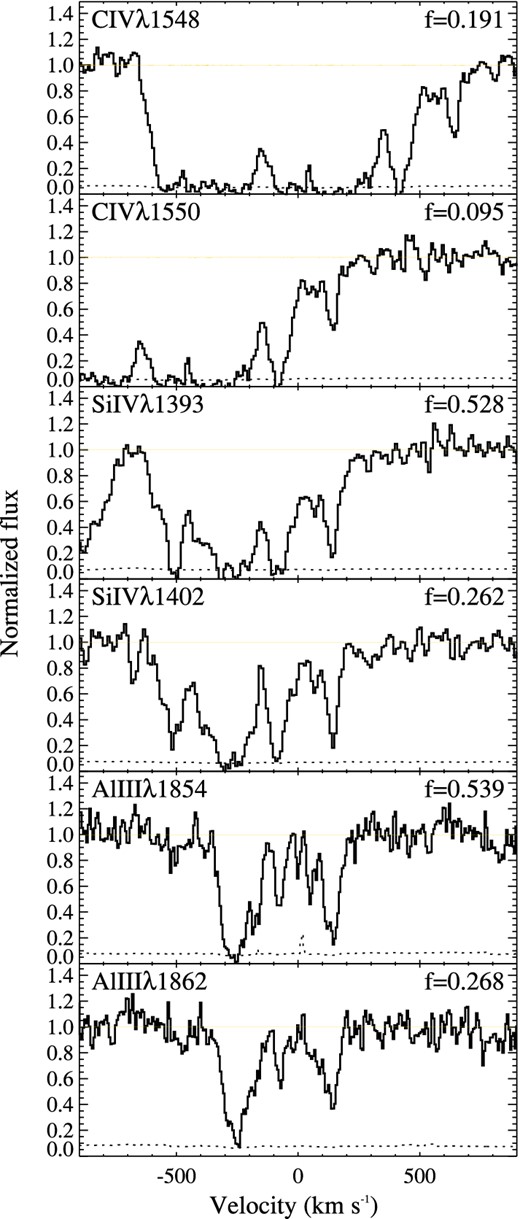
High-ionization lines. These lines are highly saturated. See Fig. 2 for details.
3.2 Dust depletion
Refractory elements, such as Fe, Ni, and Cr, can be heavily depleted into dust grains (e.g. Savage & Sembach 1996; Ledoux, Srianand & Petitjean 2002, De Cia et al. in preparation), and thus can be missing from the gas-phase abundances. A first indicator of the level of depletion in the ISM is the relative abundance [Zn/Fe] (referred to as the depletion factor), because Zn is marginally if not at all depleted into dust grains, and its nucleosynthesis traces Fe. We measure [Zn/Fe] =0.85 ± 0.06. This value is among the highest for QSO-DLAs, but typical at the observed metallicity of [Zn/H] =−0.7 ± 0.1 (e.g. Noterdaeme et al. 2008, De Cia et al. in preparation). Following De Cia et al. (2013), we calculate a column density of Fe in dust-phase of log N(Fe)dust = 16.74 ± 0.17 and a dust-corrected metallicity of [Zn/H]corr = −0.6 ± 0.2, indicating that even Zn is mildly depleted in this absorber, by ∼0.1 dex. This is not surprising given the level of depletion, as also discussed by Jenkins (2009).
We also compare the observed abundances of a variety of metals (namely Zn, S, Si, Mn, Cr, Fe, and Ni) to the depletion patterns of a warm halo (H), warm disc+halo (DH), warm disc (WD) and cool disc (CD) types of environments, as defined in Savage & Sembach (1996). These are fixed depletion patterns observed in the Galaxy and calculated assuming that Zn is not depleted into dust grains. We fit the observed abundances to the depletion patterns using the method described in Savaglio (2001). We find that none of the environments are completely suitable to describe the observed abundances. The fits to CD and WD patterns are displayed in Fig. 5 (|$\chi ^{2}_\nu$|=1.18 and 1.58, respectively, with 4 degrees of freedom). For the CD, the lower limit on the Si column density is not very well reproduced, while the fit for the WD overestimates the Mn abundance. The real scenario could be somewhere in between these two environments. Alternatively, the actual depletion pattern is different than what has been observed by Savage & Sembach (1996), or there are some nucleosynthesis effects which we cannot constrain for our case.

The dust-depletion pattern fit for a cold disc (red solid curve) and a WD (red dashed curve) to the observed abundances measured from absorption-line spectroscopy (diamonds and arrows, for the constrained and 3σ limits, respectively).
Another quantity that is very useful to derive from the observed dust depletion is the dust-to-metals ratio (DTM, normalized by the Galactic value). Constraining the DTM distribution on a variety of environments can indeed shed light on the origin of dust (e.g. Mattsson et al. 2014). Based on the observed [Zn/Fe] and following De Cia et al. (2013), we calculate DTM =1.01 ± 0.03, i.e. consistent with the Galaxy. From the depletion-pattern fit described above we derive similar, although somewhat smaller, DTM =0.84 ± 0.02 (CD) and DTM =0.89 ± 0.02 (WD). These values are in line with the distribution of the DTM with metallicity and metal column densities reported by De Cia et al. (2013), and are also consistent with those of Zafar & Watson (2013). Following Zafar & Watson (2013), we calculate DTM =0.1 now based on the dust extinction AV that we model from the SED fit (Section 3.9). Due to the small amount of reddening in the SED, this DTM(AV) value is a factor of 10 lower than expected at the metal column densities observed. This will be discussed further in Section 4.3.
At the metallicity of GRB 121024A (∼1/3 solar), it is not possible to draw further conclusions on the dust origin based on the DTM. Both models of pure stellar dust production and those including dust destruction and grain growth in the ISM converge to high (Galactic-like) DTM values at metallicities approaching solar (Mattsson et al. 2014).
3.3 Distance between GRB and absorbing gas
The most likely origin of the fine-structure transitions observed in the a+b (α+β) component, is photoexcitation by UV photons from the GRB afterglow itself (see e.g. Prochaska, Chen & Bloom 2006; Vreeswijk et al. 2007). Assuming the afterglow to be the only source of excitation, we model the population of the different levels of Fe and Ni, closely following Vreeswijk et al. (2013). Using an optical light curve to estimate the luminosity of the afterglow, we can then determine how far the excited gas must be located from the GRB site, for the afterglow to be able to excite these levels. We model the total column density from component a+b (α+β) of all observed levels (ground state and excited states) of Ni ii and Fe ii. We input the optical light curve from Skynet, see Fig. 6 and tables in Appendix A, which is extrapolated to earlier times using the power-law decay observed. We use the broadening parameters b derived from the Voigt-profile fits, and the same atomic parameters (see Vreeswijk et al. 2013).
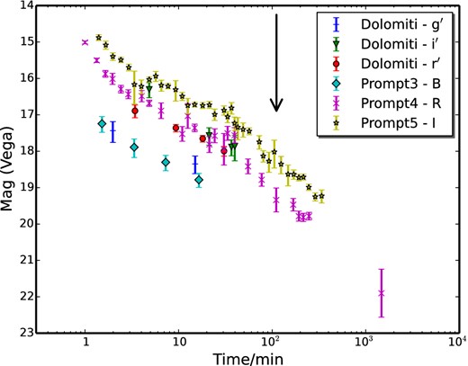
GRB-afterglow light curve from the Skynet instruments, used as input for the population modelling. The legend gives the instrument and observational band. The black arrow indicates the starting point of the X-shooter observations. Observations started 55 s after the GRB trigger.
The best fit (see Fig. 7) is obtained with a distance of 590 ± 100 pc between the cloud and burst, and a cloud size of <333 pc (1σ). The resultant fit is rather poor (χ2/d.o.f=40.6/4). As can be seen in Figs 2 and 3, the column densities of the ground level of Ni ii (as probed by Ni ii λλλ 1709, 1454, 1467) and fifth excited level of Fe ii (as probed by Fe ii 5s λλ 1559, 2360) are not very well constrained due to the observed spectrum having a low S/N ratio near those features. The formal errors from the Voigt profile fit are likely an underestimate of the true error for these column densities. This, in turn, results in the χ2 of the excitation model fit being overestimated. Furthermore, the lack of spectral time series means the resultant parameters are not well constrained. For the c+d+e component, we are able to set a lower limit of 1.9 kpc on the distance to the burst using Fe ii, and 3.5 kpc using Si ii (3σ). Since Si ii is saturated, we use the EW to determine the column density, but that only gives the total value of all components together. Hence, for the c+d+e component we fitted using vpfit and compared the total column density with what we get from the EWs. After establishing that both methods yield the same result, we feel confident in using the column density of logN(Si ii)c + d + e > 15.99 together with a detection limit logN(Si ii*)c + d + e < 12.80 on the 1265 Å line, as this is the strongest of the Si ii* lines. The lack of vibrationally excited H2 in the spectra, see below, is in agreement with a distance ≫100 pc, see Draine (2000).
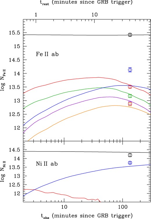
Best-fitting model for the excited-level populations of the a+b (α+β) column densities of Fe ii (top panel) and Ni ii (bottom). Black lines show the fit to the resonance level. For Fe ii, from the lower levels and up, excited-level population are shown with red, green, purple, orange and blue. For Ni ii, the red line shows the first excited level, while the blue line shows the second. Open circles show the actual values from Voigt-profile fits.
3.4 Molecular hydrogen
We detect Lyman- and Werner-band absorption lines of molecular hydrogen at redshift z = 2.3021 (corresponding to metal-line component ‘c+d+e’) in rotational levels J =0, 1, 2 and 3, see Fig. 8. The fitting and analysis of the molecular hydrogen transition lines follow Ledoux et al. (2002), Ledoux, Petitjean & Srianand (2003) and Krühler et al. (2013). We performed a Voigt-profile fit of lines mainly from the Lyman bands L0–0 up to L3–0, as these are found in the less noisy part of the spectrum (a few J = 2 and 3 lines from the Lyman bands L4–0 and L5–0 were also fitted). J = 0 and 1 lines are strong and fairly well constrained by the presence of residual flux around them, hinting at damping wings in L ≥ 1. Given the low spectral resolution of the data and the possibility of hidden saturation, we tested a range of Doppler parameters. The estimated H2 column densities, log N(H2) are given in Table 6 for Doppler parameter values of b = 1 and 10 km s−1 resulting in log N(H2) = 19.8–19.9. Using the column density of neutral hydrogen for component ‘c+d+e’ of log |$N({\rm H\,\,\small {I}})=21.6$|, calculated assuming the same Zn metallicity for the two main velocity components (‘a+b’ and ‘c+d+e’), this results in a molecular fraction of the order of log f ∼ −1.4, where f ≡ 2N(H2)/(N(H i)+2N(H2)). For the component ‘a+b’ at redshift z ∼ 2.2987, we report log N(H2) < 18.9 as a conservative upper limit on detection. A more detailed analysis is not possible because of the high noise-level. The implications of this detection are discussed in Section 4.4.
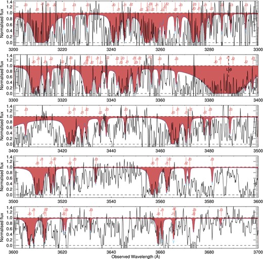
X-shooter spectrum showing Lyman- and Werner-band absorption. The shaded area shows the synthetic spectrum from a fit with Doppler parameter b = 1 km s−1, while the blue-dotted line shows the fit for b = 10 km s−1. J0 marks the transitions from the J = 0 rotational level, and likewise for higher J.
Estimated column densities for H2 for broadening parameter values b = 10 and 1 (km s−1).
| Rotational level | log(N(H2)/cm−2) | |
|---|---|---|
| b = 10 km s−1 | b = 1 km s−1 | |
| J = 0 | 19.7 | 19.7 |
| J = 1 | 19.2 | 19.3 |
| J = 2 | 16.1 | 18.3 |
| J = 3 | 16.0 | 18.2 |
| Total | 19.8 | 19.9 |
| Rotational level | log(N(H2)/cm−2) | |
|---|---|---|
| b = 10 km s−1 | b = 1 km s−1 | |
| J = 0 | 19.7 | 19.7 |
| J = 1 | 19.2 | 19.3 |
| J = 2 | 16.1 | 18.3 |
| J = 3 | 16.0 | 18.2 |
| Total | 19.8 | 19.9 |
We searched for vibrationally excited H2 by cross-correlating the observed spectrum with a theoretical model from Draine (2000) and Draine & Hao (2002) similar to the procedure outlined in Krühler et al. (2013). There is no evidence for H|$_{2}^{*}$| in our data, neither through the cross-correlation nor for individual strong transitions, and we set an upper limit of 0.07 times the optical depth of the input model. This approximately corresponds to log N(H|$_{2}^{*})<15.7$|. A column density of H|$_2^*$| as high as seen in e.g. GRBs 120815A or 080607 (Sheffer et al. 2009) would have been clearly detected in our data.
We furthermore note that CO is not detected. We set a conservative limit of log N(CO) < 14.4, derived by using four out of the six strongest CO AX bandheads with the lowest six rotational levels of CO. The wavelength range of the other two bandheads are strongly affected by metal lines, and thus do not provide constraining information.
3.5 Emission lines
In the NIR spectrum, we detect Hα, Hβ, the [O ii] λλ3727, 3729 doublet, [N ii] λ6583 (highest redshift [N ii] detection published for a GRB host) and the two [O iii] λλ4959, 5007. Table 7 shows the fluxes (extinction-corrected, see Section 3.8). The reported fluxes are derived from Gaussian fits, with the background tied between the [O iii] doublet and Hβ, and between Hα and [N ii], assuming a slope of the afterglow spectrum of 0.8. [O ii] is intrinsically a doublet, so we fit a double Gaussian with a fixed wavelength spacing based on the wavelength of the rest-frame lines. Using the GROND photometry, we estimate a slit-loss correction factor of 1.25 ± 0.10. Fig. 9 shows the emission-line profiles, the 2D as well as the extracted 1D spectrum. The figure shows a Gaussian fit to the lines, after subtracting the PSF for the continuum (done by fitting the spectral trace and PSF as a function of wavelength locally around each line, see Møller 2000, for details). For the weaker [N ii], a formal χ2 minimization is done by varying the scale of a Gaussian with fixed position and width. The noise is estimated above and below the position of the trace (marked by a horizontal dotted line in Fig. 9). We assign the zero-velocity reference at the redshift of the [O iii] λ5007 line. For the weaker [N ii] line, we fix the Gaussian-profile fit to be centred at this zero-velocity.
![Emission lines detected from the GRB 121024A host. Each panel shows the 2D spectrum after continuum PSF subtraction on top. The bottom part shows the extracted 1D spectrum. The blue line shows the Gaussian fit to the line profile. The abscissa shows the velocity dispersion with respect to the [O iii] λ5007 reference frame. The [N ii] spectrum has been smoothed and binned differently than the other lines, and the fit has been performed with the Gaussian profile centre frozen at 0 km s−1 with respect to the reference frame, as indicated with the dashed line in the figure. [O ii] has been fit as a doublet for the flux estimate.](https://oup.silverchair-cdn.com/oup/backfile/Content_public/Journal/mnras/451/1/10.1093/mnras/stv960/2/m_stv960fig9.jpeg?Expires=1750435483&Signature=GDUQdHIUHwwt7-UeeFXTlPKkNe-eqdMe-VSVn2CS6TsM-Si5W1IWHnrbNe6eLG1nW6N46bb~0VQzsCoUJkMfY7ZmgLPWHL2YcUX5nfX2no~K-ED8fSjmqOricG87UoaOSu9nClMr3BfZKUL~EgsDwiaJ7JTCePkAZu4OAkQIS3T1ev~sb1M0RP1Dznu~2d-jIVtqQOvhXDm4nl-25-tCnpJGRPNJcuetsc8FJC07PM6wK44~9nPJT-yp19-XuQzQVBU--v2gGrmCkXeHK3bLsXo5azkpNyCNMM~Iw9HT6OpzXMsVf8vlHSNLcaCQaIchKL5Cpd6gDqW00hMFbkrHzA__&Key-Pair-Id=APKAIE5G5CRDK6RD3PGA)
Emission lines detected from the GRB 121024A host. Each panel shows the 2D spectrum after continuum PSF subtraction on top. The bottom part shows the extracted 1D spectrum. The blue line shows the Gaussian fit to the line profile. The abscissa shows the velocity dispersion with respect to the [O iii] λ5007 reference frame. The [N ii] spectrum has been smoothed and binned differently than the other lines, and the fit has been performed with the Gaussian profile centre frozen at 0 km s−1 with respect to the reference frame, as indicated with the dashed line in the figure. [O ii] has been fit as a doublet for the flux estimate.
Measured emission-line fluxes.
| Transition | Wavelengtha | Fluxb | Widthc | Redshift |
|---|---|---|---|---|
| |$[{O\,{\small II}}]$| | 3726.03, 3728.82 | 14.5 ± 1.2 | –d | 2.3015e |
| Hβ | 4861.33 | 7.4 ± 0.4 | 218 ± 12 | 2.3012 |
| |$[{O\,{\small III}}]$| | 4958.92 | 9.0 ± 0.4 | 194 ± 28 | 2.3017 |
| |$[{O\,{\small III}}]$| | 5006.84 | 27.2 ± 0.7 | 192 ± 7 | 2.3010 |
| Hα | 6562.80 | 21.0 ± 1.5 | 279 ± 17 | 2.3010 |
| |$[{N\,{\small II}}]$| | 6583.41 | 1.9 ± 0.7 | ∼140 | 2.3015f |
Notes.aWavelengths in air in units of Å.
bExtinction corrected flux in units of 10−17 erg s−1 cm−2.
cFWHM of line (after removing instrumental broadening) in units of km s−1. Errors do not include uncertainty in continuum.
d[O ii] is intrinsically a doublet, which is not fully resolved here, so we do not give the width.
eCalculated using a weighted wavelength average of 3727.7 Å.
fThe Gaussian fit shown of [N ii] has a redshift frozen to that of the [O iii] λ5007 line.
3.6 Star formation rate
The SFR can be derived from the emission line fluxes of Hα and [O ii]. Using conversion factors from Kennicutt (1998), but converted from a Salpeter initial mass function (IMF) to Chabrier (Treyer et al. 2007), we report extinction corrected (see Section 3.8) values of SFRHα = 42 ± 11 M⊙ yr−1 from the Hα flux and an |${\rm SFR}_{[{O\,{\small II}}]}=53\pm 15$| M⊙ yr−1 derived from [O ii]. For a comparison with results from the stellar population synthesis modelling see Section 3.10.
3.7 Metallicity from emission lines
We determine the gas-phase metallicity of the GRB host galaxy using the strong-line diagnostics R23 (using the ratio ([O ii] λλ3727 + [O iii] λλ4959, 5007)/Hβ), O3N2 (using ([O ii]/Hβ)/([N ii]/Hα)) and N2 (using [N ii]/Hα; for a discussion of the different diagnostics see e. g. Kewley & Ellison 2008). Note that different metallicity calibrators give different values of metallicity. R23 appears to be consistently higher than O3N2 and N2. The R23 diagnostic has two branches of solutions, but the degeneracy can be broken using the ratios [N ii]/Hα or [N ii]/[O ii]. In our case [N ii]/Hα = 0.09±0.02 and [N ii]/[O ii] = 0.13 ± 0.03, which places the R23 solution on the upper branch (though not far from the separation). Because of the large difference in wavelength of the emission lines used for R23, this method is sensitive to the uncertainty on the reddening. Both O3N2 and N2 use lines that are close in wavelength, so for these we expect the reddening to have a negligible effect. Instead, they then both depend on the weaker [N ii] line, which has not got as secure a detection. We derive 12 + log(O/H) = 8.6 ± 0.2 for R23 (McGaugh 1991), 12 + log(O/H) = 8.2 ± 0.2 for O3N2 and 12 + log(O/H) = 8.3 ± 0.2 for N2 (both from Pettini & Pagel 2004). The errors include the scatter in the relations (these values are from Kewley & Ellison 2008, and references therein), though the scatter in N2 is likely underestimated. See Section 4.1 for a comparison with absorption-line metallicity.
3.8 Balmer decrement
The ratio of the Balmer lines Hα and Hβ can be used to estimate the dust extinction. We use the intrinsic ratio found I(Hα)/I(Hβ) = 2.86 (Osterbrock 1989), for star-forming regions (and case B recombination, meaning photons above 13.6 eV are not re-absorbed), where we expect GRBs to occur. The ratio we measure is 2.98 which, assuming the extinction law of Calzetti et al. (2000),3 results in E(B − V) = 0.04 ± 0.09 mag. We note that adopting a different extinction law (from e.g. Pei 1992) results in the same reddening correction within errors, because there is little difference within the wavelength range of the Balmer lines.
3.9 Broad-band SED
We fitted the broad-band afterglow data from XRT and GROND (without the g′-band, due to possible DLA contamination), where simultaneous data exist (11 ks after the trigger). The fit was performed within the isis software (Houck & Denicola 2000) following the method of Starling et al. (2007). The XRT data were extracted using Swift tools. We use single and broken power-law models. For the broken power law, we tie the two spectral slopes to a fixed difference of 0.5. Such spectral feature is known as the cooling break of GRB afterglows (e.g. Sari 1998), and is observed to be the best-fitting model for most burst Zafar et al. (2011), with the exception of GRB 080210 (De Cia et al. 2011; Zafar et al. 2011). We fit with two absorbers, one Galactic fixed at |$N({\rm H})_{{\rm X}}^{{\rm Gal}}=7.77\times 10^{20}$| cm−2 (Willingale et al. 2013), and one intrinsic to the host galaxy.4 An Small Magellanic Cloud (SMC) dust-extinction model (the average extinction curve observed in the SMC) was used for the host, while the reddening from the Milky Way (MW) was fixed to E(B − V) = 0.123 (Schlegel, Finkbeiner & Davis 1998). A single power law is preferred statistically (χ2 / d.o.f = 1.07), see Fig. 10, but the two models give similar results.
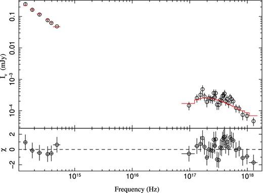
NIR-to-X-ray SED and model for the afterglow at 11 ks after the trigger. The solid red line shows the model. g′-band magnitude is not included in the fit, due to possible contribution from the Lyα transition.
The best-fitting parameters for the single power-law SMC absorption model are |$N({\rm H})_{\rm X}=(1.2^{+0.8}_{-0.6})\times 10^{22}$| cm−2 and E(B − V) =0.03 ± 0.02 mag at a redshift of z = 2.298, and a power-law index of β = 0.90 ± 0.02 (90 per cent confidence limits), see Table 8. Large Magellanic Cloud (LMC) and MW (the average extinction curves observed in the LMC and the MW) model fits result in the same values within errors. For a discussion on the extinction see Section 4.3.
Best-fitting parameters from the broad-band SED, for a single power-law SMC absorption model.
| N(H)X | |$(1.2^{+0.8}_{-0.6})\times 10^{22}$| cm−2 |
| E(B − V) | 0.03 ± 0.02 mag |
| Power-law index β | 0.90 ± 0.02 |
| N(H)X | |$(1.2^{+0.8}_{-0.6})\times 10^{22}$| cm−2 |
| E(B − V) | 0.03 ± 0.02 mag |
| Power-law index β | 0.90 ± 0.02 |
3.10 Stellar population synthesis modelling
Using our photometry of the host, see Table 3, we perform stellar population synthesis modelling of the host galaxy. We use a grid of stellar evolution models with different star formation time-scales, age of stellar population and extinction, to compute theoretical magnitudes and compare them to the observed photometry. For the model input, we assume stellar models from Bruzual & Charlot (2003), based on an IMF from Chabrier (2003) and a Calzetti dust attenuation law (Calzetti et al. 2000). Table 9 lists the galaxy parameters resulting from the best-fitting to the HAWK-I, NOT and GTC data. The best fit is obtained with a χ2 = 8 for the seven data points used in the modelling. Most of the contribution to the χ2 comes from the B-band observations. This data point lies ≈ 3σ above the best-fitting and the g-band measurement, which probes a very similar wavelength range. The reported value of the SFR takes into account the uncertainty in the dust attenuation, and thus has large error bars. We observe a significant Balmer break, which is well fitted with starburst ages between 50 and 500 Myr. The SFR of ∼40 M⊙ yr−1 is consistent with the results from Section 3.6.
Host galaxy parameters from stellar population synthesis modelling.
| Starburst age (Myr) | ∼250 |
| Extinction (mag) | 0.15 ± 0.15 |
| MB | −22.1 ± 0.2 |
| log (M*/M⊙) | |$9.9^{+0.2}_{-0.3}$| |
| SFR (M⊙ yr−1) | |$40^{+80}_{-25}$| |
| Starburst age (Myr) | ∼250 |
| Extinction (mag) | 0.15 ± 0.15 |
| MB | −22.1 ± 0.2 |
| log (M*/M⊙) | |$9.9^{+0.2}_{-0.3}$| |
| SFR (M⊙ yr−1) | |$40^{+80}_{-25}$| |
3.11 Kinematics
The X-shooter spectrum contains information both on the kinematics of the absorbing gas along the line of sight to the location of the burst inside the host galaxy, as well as kinematics of the emitting gas in H ii regions probed by the emission lines. The emission lines have a full width at half-maximum (FWHM) of around 210 km s−1 from a Gaussian fit, see Table 7. We do not observe signs of rotation in the two-dimensional spectrum. One possibility is that the galaxy could be dominated by velocity dispersion, as observed for galaxies of similar mass and properties (Förster et al. 2009). The velocity width that encloses 90 per cent of the optical depth (as defined by Ledoux et al. 2006) is 460 km s−1 based on the Si ii λ1808 line. This is consistent with the correlation between absorption line width and metallicity for GRB host galaxies of Arabsalmani et al. (2015). The velocity for each absorption component, with respect to the emission lines, is given in Table 4. The characteristics of different gas components are discussed in Section 4.5.
3.12 Intervening systems
We identify three intervening systems along the line of sight, at redshifts z = 2.0798, 1.959, and 1.664. Table 10 lists the observed lines along with the measured EWs. Furthermore only at z = 1.959 do we observe the Lyα line, but blended with a Si iv line. The intervening systems will not be discussed further in this work.
EWs of intervening systems.
| EWs/Å | |||
|---|---|---|---|
| Transition | z = 2.0798 | z = 1.959 | z = 1.664 |
| C iv, λ1548 | 0.43 ± 0.10 | 3.64 ± 0.15 | – |
| C iv, λ1550 | 0.38 ± 0.10 | 3.11 ± 0.14 | – |
| Fe ii, λ2382 | – | 0.72 ± 0.10 | 0.36 ± 0.05 |
| Mg ii, λ2796 | – | 3.73 ± 0.08 | 1.29 ± 0.05 |
| Mg ii, λ2803 | – | 2.53 ± 0.11 | 1.02 ± 0.05 |
4 DISCUSSION AND IMPLICATIONS
4.1 Abundance measurements from absorption and emission lines
The metallicity of GRB hosts is usually determined either directly through absorption line measurements, or via the strong-line diagnostics using nebular-line fluxes. The two methods probe different physical regions; the ISM of the host galaxy along the line of sight as opposed to the ionized star-forming H ii regions emission – weighted over the whole galaxy. Hence, the two methods are not necessarily expected to yield the same metallicity, see for instance Jorgenson & Wolfe (2014). The line of sight towards the GRB is expected to cross star-forming regions in the GRB host. Thus, the absorption and emission lines may probe similar regions. Local measurements from the solar neighbourhood show a concurrence of the two metallicities in the same region, see e. g. Esteban et al. (2004). Only a few cases where measurements were possible using both methods have been reported for QSO-DLAs (see e.g. Bowen et al. 2005; Jorgenson & Wolfe 2014) but never for GRB-DLAs. The challenge is that the redshift has to be high enough (z ≳ 1.5) to make Lyα observable from the ground, while at the same time the host has to be massively star forming to produce sufficiently bright emission lines. Furthermore, the strong-line diagnostics are calibrated at low redshifts, with only few high redshift cases available (see for instance Christensen et al. 2012).
The spectrum of GRB 121024A has an observable Lyα line as well as bright emission lines. We find that the three nebular line diagnostics R23, O3N2 and N2 all find a similar oxygen abundance of 12 + log(O/H) = 8.4 ± 0.4. Expressing this in solar units, we get a metallicity of [O/H] ∼−0.3 (or slightly lower if we disregard the value found from the R23 diagnostic, given that we cannot convincingly distinguish between the upper and lower branch). This is indeed consistent with the absorption line measurement from the low-depletion elements (dust-corrected value) [Zn/H]corr = −0.6 ± 0.2, though the large uncertainty in the strong-line diagnostics hinders a more conclusive comparison.
Krogager et al. (2013) find a slightly lower metallicity from absorption lines in the spectrum of quasar Q2222-0946, compared to the emission-line metallicity. However, this is easily explained by the very different regions probed by the nebular lines (6 kpc above the galactic plane for this quasar) and the line of sight, see also Péroux et al. (2012). QSO lines of sight intersect foreground galaxies at high-impact parameters, while the metallicity probed with GRB-DLAs are associated with the GRB host galaxy. Interestingly, Noterdaeme et al. (2012) find different values for the metallicities, even with a small impact parameter between QSO and absorber, for a QSO-DLAs. A comparison of the two metallicities is also possible for Lyman break galaxies (LBGs), see for instance Pettini et al. (2002) for a discussion on the metallicity of the galaxy MS 1512–cB58. They find that the two methods agree for a galaxy with an even larger velocity dispersion in the absorbed gas than observed here (∼1000 km s−1). The line of sight towards GRB 121024A crosses different clouds of gas in the host galaxy, as shown by the multiple and diverse components of the absorption-line profiles. The gas associated with component a+b is photoexcited, indicating that it is the closest to the GRB. Given the proximity, the metallicity of this gas could be representative of the GRB birth site. Assuming the GRB exploded in an H ii region, the emission- and absorption-metallicities are expected to be similar, though if other H ii region are dominating the brightness, the GRB birth sight might contribute only weakly to the emission line-flux, see Section 4.5. Building a sample of dual metallicity measurements will increase our understanding of the metallicity distribution and evolution in galaxies.
4.2 The mass–metallicity relation at z ∼ 2
4.3 Grey dust extinction?
We determine the dust extinction/attenuation of the host galaxy of GRB 121024A both from the Balmer decrement (Section 3.8) and a fit to the X-ray and optical spectral energy distribution (SED, see Section 3.9), as well as from the stellar population synthesis modelling (Section 3.10). The first method determines the attenuation of the host H ii regions (from the X-shooter spectrum alone), while the SED fitting probes the extinction along the line of sight (using XRT+GROND data). The stellar population synthesis modelling models the host attenuation as a whole (using host photometry). All methods determine the amount of extinction/attenuation by comparing different parts of the spectrum with known/inferred intrinsic ratios, and attribute the observed change in spectral form to dust absorption and scattering. We find values that agree on a colour index E(B − V) ∼ 0.04 mag. This value is small, but falls within the range observed for GRB-DLA systems. However, low AV's are typically observed for the lowest metallicities. For our case, we would expect a much higher amount of reddening at our determined H i column density and metallicity. Using the metallicity of [Zn/H]corr = −0.6 ± 0.2, column density log |$N({\rm H\,{\small I}})=21.88\pm 0.10$|, DTM=1.01 ± 0.03 (see Section 3.2), and a reference Galactic DTM |$A_{V, \rm {Gal}}/N_{(H, \rm {Gal})}=0.45\times 10^{-21}$| mag cm2 (Watson 2011), we expect an extinction of AV = 0.9 ± 0.3 mag (De Cia et al. in preparation and Savaglio, Fall & Fiore 2003). This is incompatible with the determined reddening, as it would require RV > 15 (RV for the Galaxy is broadly in the range 2–5). For the Balmer decrement and SED fitting, we have examined different extinction curves (MW and LMC besides the SMC) and we have tried fitting the SED with a cooling break, neither option changing the extinction significantly. In an attempt to test how high a fitted reddening we can achieve, we tried fitting the SED with a lower Galactic |$N({\rm H\,{\small I}})$| and reddening. While keeping reasonable values (it is unphysical to expect no Galactic extinction at all), and fitting with the break, the resulting highest colour index is E(B − V) ∼ 0.06 mag. This is still not compatible with the value derived from the metallicity, so this difference needs to be explained physically.
One possibility to consider is that the host could have a lower DTM, and hence we overestimate the extinction we expect from the metallicity. However, we see no sign of this from the relative abundances, see Section 3.2. The metallicity is robustly determined from Voigt-profile fits and EW measurement of several lines from different elements (including a lower limit from the none Fe-peak element Si). The lines are clearly observed in the spectra, see Fig. 2, and the metallicity that we find is consistent with the mass–metallicity relation.
To examine the extinction curve, we perform a fit to the XRT (energy range: 0.3–10 keV) X-ray data alone and extrapolate the resultant best-fitting power law to optical wavelengths. We try both a single power law, as well as a broken power law with a cooling break in the extrapolation. The latter is generally found to be the best model for GRB extinction in optical fit (e.g. Greiner et al. 2011; Zafar et al. 2011; Schady et al. 2012). We calculate the range of allowed Aλ by comparing the X-shooter spectrum to the extrapolation, within the 90 per cent confidence limit of the best-fitting photon index, and a break in between the two data sets (X-ray and optical). The resulting extinction does not redden the afterglow strongly, so we cannot constrain the total extinction very well directly from the SED. However, the optical spectroscopy indicates a high metal column density. The strong depletion of metals from the gas phase supports the presence of dust at AV = 0.9 ± 0.3 mag (see Section 3.2). Fixing AV at this level, allows us to produce a normalized extinction curve (Fig. 11). This extinction curve is very flat, much flatter than any in the Local Group (Fitzpatrick & Massa 2005), with an RV > 9.
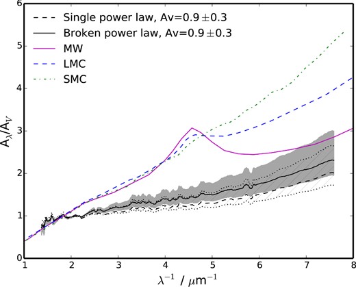
Extinction curves for the line of sight to GRB 121024A. We plot the extinction law assuming AV = 0.9 ± 0.3 mag as expected from the measured metallicity, H i column density and DTM. The solid black curve shows the extinction curve for a broken power law with AV = 0.9, while the grey-shaded area corresponds to the AV error-space. Likewise, the extinction curve for a single power law is plotted with the dashed black curve, and the hatched area displays the error-space. Overplotted, in colours, are extinction curves from Pei (1992).
The most likely physical scenario that can explain this shape of the curve is grey dust. If the dust extinction is ‘grey’, i.e. has a much weaker dependence on wavelength than in the local extinction laws, then a given visual extinction will be much less apparent in the SED (‘flat’ extinction curve) and thus underestimated in our analysis. Such grey extinction corresponds to larger RV and is physically interpreted with large grain sizes. A weak wavelength dependence in the extinction for GRBs has been suggested before. Savaglio & Fall (2004) reported an MW-like depletion pattern, but a very low reddening in the SED. Gao, Jiang & Li (2008) likewise claim a grey extinction law for GRB lines of sight determined by comparing observed spectra to intrinsic ones (by extrapolating from X-rays), arguing for grain growth through coagulation in the dense molecular clouds surrounding GRBs. The larger grains have an extinction that is less dependent on wavelength, because of the contribution of their physical cross-section to the opacity. Preferable destruction of the smaller grains by the GRB would be another possibility, but is unlikely in our case, because the absorbing gas is far from the GRB. We note that the other GRB-DLAs with molecular-hydrogen detection show the expected amount of reddening (using a standard extinction curve), though anomalies do exist in GRB observations. The most notable example to date is reported by Perley et al. (2008) for GRB 061126. As for the GRB 121024A afterglow, they observe a very flat optical-to-X-ray spectral index, arguing for large quantities of grey dust, or a separate origin of the optical and X-ray afterglow. To fit the extinction curve for GRB 061126, an RV ∼ 10 is needed. We find an RV even higher than this, making this case even more extreme than previously observed. We refer to future work on this problem (Friis et al., in preparation), as a deeper analysis is beyond the scope of this paper.
4.4 Molecular hydrogen in GRB-DLAs
The lack of detection of molecular hydrogen towards GRBs has puzzled astronomers (see e. g Tumlinson et al. 2007), given that long GRBs are associated with active star formation, and hence are expected to show signatures of molecular clouds. Compared to QSO-DLA line of sights then, we would expect the presence of H2 to be more common for GRB-DLAs, because the QSO-DLA line of sights have a higher probability to intersect the outskirts/halo of the intervening galaxy, where we would anticipate a low molecular content. Recently, a number of H2 detections in GRB afterglows have been reported (Prochaska et al. 2009; Krühler et al. 2013; D'Elia et al. 2014), making GRB121024A the fourth definite case. This detection supports the emerging picture that dust has played a major role in biasing past observations against molecular detection (e.g. Ledoux et al. 2009). Molecules are thought to form on the surface of dust grains, and once formed, shielded from Lyman–Werner photons by the grains. Krühler et al. (2013) suggest that it is likely this connection that is responsible for the low number of H2 detections towards GRB-DLAs. The high dust column density makes the GRB afterglow UV-faint, preventing high-resolution and high S/N spectroscopy, which is needed to identify the presence of molecular gas. Thus, the lack of H2 detections in most GRB-DLAs can be explained with an observational bias. They illustrate this argument by investigating the metallicity, N(H i) and dust depletion parameter space, showing that the GRB-DLAs with unsuccessful molecular searches fall outside the region where we would expect detections (with the only exception being GRB 050829A). This argument is supported by the observed log |$N({\rm H\,{\small I}})$|, metallicity and depletion factor of GRB 121024A, which lies inside the parameter space where molecular detections are expected.
The high level of dust depletion observed in this GRB-DLA (see Section 3.2), is consistent with molecular detections in QSO-DLAs (Noterdaeme et al. 2008; Krühler et al. 2013), where there is a strong preference for H2-bearing DLAs to have significant depletion factors. The dependence on the total neutral hydrogen column density is weak (although intrinsically weak molecular lines are better constrained in strong DLAs), whereas the parameter that seems to determine whether H2 is detected, is the column density of iron locked into dust. The log N(Fe)dust that we measure is 2 dex higher than the column density above which a significant presence of molecules has been observed in QSO-DLAs (Noterdaeme et al. 2008). Indeed De Cia et al. (2013) studied log N(Fe)dust and concluded that GRB hosts are promising sites for molecular detections.
D'Elia et al. (2014) find a molecular fraction for GRB 120327A of log(f) between −7 and −4 with a depletion factor of [Zn/Fe] = 0.56 ± 0.14, while for the dustier line of sight towards GRB 120815A, Krühler et al. (2013) reports a value of log(f) = −1.14 ± 0.15 ([Zn/Fe] = 1.01 ± 0.10). For GRB 121024A we find intermediate values, although with the high noise-level the numbers are consistent with those reported for GRB 120815A. For GRB 080607, Prochaska et al. (2009) only report limits on both the molecular fraction and the Zn+Fe column densities. Although the sample is too small to infer anything statistically, it appears that the H2 detection criteria in GRB afterglows follow the trend observed for QSO-DLAs. For a fair estimate of the molecular fraction, the column densities of both H2 and H i should be constrained for individual velocity components, while this is hardly the case for H i. Recent work (e.g. Balashev et al. 2015) indicates that the molecular fraction in QSO-DLAs can possibly be much higher than the line-of-sight average values usually measured.
4.5 Gas kinematics: dissecting the host components
One of the striking features of the metal absorption-line profiles observed towards GRB 121024A is that they consist of two widely separated groups of velocity components (a+b and c+d+e, see Section 3.1). The separation is of about 340 km s−1, which lies at the high end of the velocity distribution of Møller et al. (2013) and Ledoux et al. (2006). The latter is for QSO-DLAs, however Arabsalmani et al. (2015) showed that GRB-DLAs follow the velocity–metallicity distribution of QSO-DLAs. This suggests that either the two components belong to separate galaxies (see for instance Savaglio et al. 2012, on the GRB 090323 systems), or that this galaxy is fairly massive compared to the average GRB host of ∼109M⊙ (Savaglio, Glazebrook & Le Borgne 2009; Castro Cerón et al. 2010, but see also Perley et al. 2013 and Hunt et al. 2014). The scenario with separate galaxies is disfavoured, because the two absorption components show very similar relative abundances (see Table 4) and also because the emission lines are centred in between the two absorption components (unlike for GRBs 050820A and 060418; see Chen 2012). Thus, a likely possibility is that the two absorption components are probing different regions within the host. This is in agreement with the mass found in Section 3.10, of almost 1010 M⊙.
Furthermore, the blue (a+b) and the red (c+d+e) absorption components are associated with gas at different physical conditions. On one hand, Fe ii, Ni ii and Si ii fine-structure lines are detected only in the blue component. These lines are photoexcited by the GRB radiation at a distance of ∼600 pc. On the other hand, H2 molecules are detected in the red component only, indicating a gas that is not disturbed by the GRB (at a distance of minimum 3.5 kpc). Through absorption-line spectroscopy at the X-shooter resolution, these two different gas components could be located inside the host (with respect to the GRB) and characterized.
The observed emission component (arbitrarily set at v = 0) traces the brightest star-forming regions. Since GRBs tend to reside around the brightest star-forming regions in their host (Fruchter et al. 2006), one might expect to observe absorption components at velocities close to that of the emission as the line of sight passes through this gas. However, the gas around the GRB can be photoionized out to hundreds of parsecs (e.g. Ledoux et al. 2009; Vreeswijk et al. 2013); it is thus highly unlikely that the optical/UV absorption lines are probing the actual GRB environment. For GRB 121024A, this is further supported by the fact that the a,b component is located ∼600 pc away from the GRB. Given that giant molecular clouds have a maximum radius of ∼200 pc (Murray 2011), the a,b component is undoubtedly unrelated to the GRB surroundings.
Although GRBs are most often associated with the brightest star-forming regions, this is not always the case. GRB 980425 (e.g. Michałowski et al. 2009) is an example where the star-forming region in which the GRB occurred is quite faint compared to the larger and brighter star-forming regions in the host. A potentially similar scenario could hold for GRB 121024A as well, in which case the burst should not be identified with v = 0. In this situation, the possible interpretations of the kinematics would be different and lead to other geometric setups compared to those conceivable were the GRB localized close to v = 0. It should also be noted that we have not discussed transverse motion which could complicate the interpretation even further. Finally, since the host is most likely an irregular galaxy, indicating a 3D perturbed environment without a rotating disc, we find it appropriate not to draw further conclusions.
While the available data do not allow us to discriminate between possible scenarios, this work demonstrates how powerful GRB afterglow observations can be to start dissecting individual building-block components of star-forming galaxies at z ∼ 2 and above. This is especially true once we have gathered enough data to compile a statistical sample; see e.g. Fox et al. (2008) for previous work on VLT/UVES data and Fynbo et al. (in preparation) for upcoming VLT/X-shooter results on a large afterglow sample.
MF acknowledges support from the University of Iceland Research fund. ADC acknowledges support by the Weizmann Institute of Science Dean of Physics Fellowship and the Koshland Center for Basic Research. The Dark Cosmology Centre is funded by the DNRF. RLCS is supported by a Royal Society Dorothy Hodgkin Fellowship. JPUF acknowledge support from the ERC-StG grant EGGS-278202. CCT is supported by a Ramón y Cajál fellowship. The research activity of J. Gorosabel, CCT, and AdUP is supported by Spanish research project AYA2012-39362-C02-02. AdUP acknowledges support by the European Commission under the Marie Curie Career Integration Grant programme (FP7-PEOPLE-2012-CIG 322307). SS acknowledges support from CONICYT-Chile FONDECYT 3140534, Basal-CATA PFB-06/2007, and Project IC120009 ‘Millennium Institute of Astrophysics (MAS)’ of Iniciativa Científica Milenio del Ministerio de Economía, Fomento y Turismo. Part of the funding for GROND (both hardware as well as personnel) was generously granted from the Leibniz-Prize to professor G. Hasinger (DFG grant HA 1850/28-1). We thank Alain Smette for providing the telluric spectrum, and the referee for very constructive feedback.
Based on observations carried out under programme ID 090.A-0088(B) with the X-shooter spectrograph installed at the Cassegrain focus of the Very Large Telescope (VLT), Unit 2 – Kueyen, operated by the European Southern Observatory (ESO) on Cerro Paranal, Chile. Also used are observations made with the Nordic Optical Telescope, operated by the Nordic Optical Telescope Scientific Association, and the Gran Telescopio Canarias (programme GTC67-13B), both at the Observatorio del Roque de los Muchachos, La Palma, Spain, of the Instituto de Astrofisica de Canarias. HAWK-I imaging used is part of the programme 092.A-0076(B). This work made use of data supplied by the UK Swift Science Data Centre at the University of Leicester.
http://www.ast.cam.ac.uk/ rfc/vpfit.html
This procedure does not aim at reproducing the observed telluric spectrum, but simply reject suspect telluric lines from the Voigt-profile fit.
We assume solar metallicity, not to provide a physical description of the absorbers, but purely to let N(H)X conform to the standard solar reference. The reference solar abundances used are from Wilms, Allen & McCray (2000).
REFERENCES
APPENDIX A: SKYNET MAGNITUDE TABLES
Tables A1 –A6 give the magnitudes (not corrected for reddening) used for the optical light-curve input to model the distance between the excited gas (component a+b) and the burst itself.
Skynet – filter R.
| Filter | Time (h) | Exposure time | S/N | Mag. (Vega) |
|---|---|---|---|---|
| R | 0.016 56 | 1 × 10 s | 27.7 | 15.01 ± 0.04 |
| R | 0.022 32 | 1 × 10 s | 18.9 | 15.51 ± 0.06 |
| R | 0.027 60 | 1 × 10 s | 12.1 | 15.88 ± 0.09 |
| R | 0.032 88 | 1 × 10 s | 7.58 | |$16.0^{+0.2}_{-0.1}$| |
| R | 0.040 32 | 1 × 20 s | 10.7 | 16.3 ± 0.1 |
| R | 0.048 24 | 1 × 20 s | 9.35 | 16.4 ± 0.1 |
| R | 0.067 20 | 1 × 40 s | 7.45 | |$16.5^{+0.2}_{-0.1}$| |
| R | 0.080 88 | 1 × 40 s | 13.1 | |$16.68^{+0.09}_{-0.08}$| |
| R | 0.108 24 | 1 × 40 s | 5.47 | 16.9 ± 0.2 |
| R | 0.182 16 | 1 × 80 s | 5.82 | 17.5 ± 0.2 |
| R | 0.208 80 | 1 × 80 s | 3.58 | 17.0 ± 0.3 |
| R | 0.247 44 | 1 × 160 s | 10.9 | 17.4 ± 0.1 |
| R | 0.355 20 | 1 × 160 s | 5.37 | 17.8 ± 0.2 |
| R | 0.405 36 | 1 × 160 s | 6.08 | 17.6 ± 0.2 |
| R | 0.509 28 | 1 × 160 s | 2.86 | |$17.9^{+0.4}_{-0.3}$| |
| R | 0.555 84 | 1 × 160 s | 6.08 | 17.5 ± 0.2 |
| R | 0.660 00 | 1 × 160 s | 5.53 | 17.6 ± 0.2 |
| R | 0.919 92 | 3 × 160 s | 5.79 | 18.4 ± 0.2 |
| R | 1.287 12 | 4 × 160 s | 6.64 | 18.79 ± 0.2 |
| R | 1.840 08 | 9 × 160 s | 3.68 | 19.3 ± 0.3 |
| R | 2.797 68 | 7 × 160 s | 6.72 | |$19.5^{+0.2}_{-0.1}$| |
| R | 3.212 40 | 7 × 160 s | 8.31 | 19.8 ± 0.1 |
| R | 3.591 84 | 7 × 160 s | 10.1 | 19.8 ± 0.1 |
| R | 4.128 24 | 12 × 160 s | 10.7 | 19.8 ± 0.1 |
| R | 4.9908 | 18 × 160 s | 7.18 | 20.0 ± 0.1 |
| R | 24.5124 | 40 × 160 s | 1.94 | |$21.9^{+0.7}_{-0.4}$| |
Skynet – filter B.
| Filter | Time (h) | Exposure time | S/N | Mag. (Vega) |
|---|---|---|---|---|
| B | 0.025 20 | 2 × 10 s | 4.98 | 17.2 ± 0.2 |
| B | 0.055 92 | 2 × 20 s | 4.22 | |$17.9^{+0.3}_{-0.2}$| |
| B | 0.121 44 | 3 × 40 s | 5.10 | 18.3 ± 0.2 |
| B | 0.274 56 | 2 × 160 s | 5.61 | 18.8 ± 0.2 |
| B | 3.870 00 | 37 × 160 s | 5.96 | 21.2 ± 0.2 |
Skynet – filter I.
| Filter | Time (h) | Exposure time | S/N | Mag. (Vega) |
|---|---|---|---|---|
| I | 0.023 28 | 1 × 5 s | 13.4 | 14.88 ± 0.08 |
| I | 0.027 84 | 1 × 5 s | 9.57 | 15.1 ± 0.1 |
| I | 0.033 12 | 1 × 10 s | 10.2 | 15.4 ± 0.1 |
| I | 0.040 32 | 1 × 20 s | 14.6 | |$15.49^{+0.08}_{-0.07}$| |
| I | 0.048 96 | 1 × 20 s | 11.8 | |$15.70^{+0.1}_{-0.09}$| |
| I | 0.056 16 | 1 × 10 s | 2.34 | |$16.2^{+0.5}_{-0.4}$| |
| I | 0.066 72 | 1 × 40 s | 5.75 | 16.2 ± 0.2 |
| I | 0.080 88 | 1 × 40 s | 15.4 | 16.03 ± 0.07 |
| I | 0.095 04 | 1 × 40 s | 7.74 | 15.9 ± 0.1 |
| I | 0.108 96 | 1 × 40 s | 7.16 | |$16.2^{+0.2}_{-0.1}$| |
| I | 0.128 64 | 1 × 80 s | 15.1 | 16.21 ± 0.07 |
| I | 0.155 04 | 1 × 80 s | 3.84 | |$16.3^{+0.3}_{-0.2}$| |
| I | 0.182 16 | 1 × 80 s | 9.82 | 16.5 ± 0.1 |
| I | 0.208 80 | 1 × 80 s | 5.14 | 16.7 ± 0.2 |
| I | 0.247 44 | 1 × 160 s | 16.3 | 16.72 ± 0.07 |
| I | 0.301 44 | 1 × 160 s | 13.3 | |$16.74^{+0.09}_{-0.08}$| |
| I | 0.355 20 | 1 × 160 s | 11.3 | |$16.73^{+0.1}_{-0.09}$| |
| I | 0.405 36 | 1 × 160 s | 6.89 | |$17.0^{+0.2}_{-0.1}$| |
| I | 0.509 28 | 1 × 160 s | 8.51 | 16.9 ± 0.1 |
| I | 0.556 32 | 1 × 160 s | 7.10 | |$17.1^{+0.2}_{-0.1}$| |
| I | 0.612 48 | 1 × 160 s | 6.87 | |$16.8^{+0.2}_{-0.1}$| |
| I | 0.660 00 | 1 × 160 s | 5.78 | 17.2 ± 0.2 |
| I | 0.715 92 | 1 × 160 s | 3.53 | 17.3 ± 0.3 |
| I | 0.815 28 | 2 × 160 s | 5.50 | 17.4 ± 0.2 |
| I | 0.947 04 | 2 × 160 s | 11.4 | |$17.45^{+0.1}_{-0.09}$| |
| I | 1.213 68 | 1 × 160 s | 5.87 | 17.7 ± 0.2 |
| I | 1.338 72 | 2 × 160 s | 6.90 | |$18.1^{+0.2}_{-0.1}$| |
| I | 1.536 72 | 2 × 160 s | 3.92 | |$18.3^{+0.3}_{-0.2}$| |
| I | 1.755 60 | 1 × 160 s | 2.80 | |$18.0^{+0.4}_{-0.3}$| |
| I | 2.075 28 | 5 × 160 s | 4.51 | |$18.4^{+0.3}_{-0.2}$| |
| I | 2.464 80 | 5 × 160 s | 3.76 | 18.6 ± 0.3 |
| I | 2.830 80 | 6 × 160 s | 8.36 | 18.64 ± 0.1 |
| I | 3.215 04 | 7 × 160 s | 12.1 | 18.72 ± 0.09 |
| I | 3.594 96 | 7 × 160 s | 13.7 | 18.71 ± 0.08 |
| I | 4.103 28 | 11 × 160 s | 12.8 | |$18.99^{+0.09}_{-0.08}$| |
| I | 4.812 00 | 12 × 160 s | 9.54 | 193 ± 0.1 |
| I | 5.631 12 | 16 × 160 s | 6.02 | 19.2 ± 0.2 |
| I | 24.31 92 | 47 × 160 s | 1.89 | |$21^{+0.7}_{-0.4}$| |
Skynet – filter g′.
| Filter | Time (h) | Exposure time | S/N | Mag. (Vega) |
|---|---|---|---|---|
| g′ | 0.033 12 | 1 × 20 s | 3.76 | 17.4 ± 0.3 |
| g′ | 0.250 32 | 1 × 80 s | 4.45 | |$18.3^{+0.3}_{-0.2}$| |
| g′ | 0.699 12 | 1 × 80 s | 2.16 | |$19.5^{0.6}_{-0.4}$| |
| Filter | Time (h) | Exposure time | S/N | Mag. (Vega) |
|---|---|---|---|---|
| g′ | 0.033 12 | 1 × 20 s | 3.76 | 17.4 ± 0.3 |
| g′ | 0.250 32 | 1 × 80 s | 4.45 | |$18.3^{+0.3}_{-0.2}$| |
| g′ | 0.699 12 | 1 × 80 s | 2.16 | |$19.5^{0.6}_{-0.4}$| |
Skynet – filter r′.
| Filter | Time (h) | Exposure time | S/N | Mag. (Vega) |
|---|---|---|---|---|
| r′ | 0.056 88 | 1 × 20 s | 6.15 | 16.9 ± 0.2 |
| r′ | 0.155 76 | 1 × 80 s | 10.6 | 17.4 ± 0.1 |
| r′ | 0.301 68 | 1 × 160 s | 11.8 | |$17.66^{+0.1}_{-0.09}$| |
| r′ | 0.509 52 | 1 × 160 s | 8.21 | 18.0 ± 0.1 |
| r′ | 0.560 88 | 1 × 80 s | 5.14 | 18.0 ± 0.2 |
Skynet – filter i′.
| Filter | Time (h) | Exposure time | S/N | Mag. (Vega) |
|---|---|---|---|---|
| i′ | 0.080 88 | 1 × 20 s | 5.22 | 16.3 ± 0.2 |
| i′ | 0.353 28 | 1 × 80 s | 4.50 | |$17.6^{+0.3}_{-0.2}$| |
| i′ | 0.612 72 | 1 × 160 s | 4.91 | 17.9 ± 0.2 |
| i′ | 0.664 08 | 1 × 80 s | 3.06 | |$17.9^{+0.4}_{-0.3}$| |
| i′ | 21.992 88 | 38 × 160 s | 1.13 | |$20.9^{+1.2}_{-0.6}$| |
