


Abstract
The Kepler space mission and its K2 extension provide photometric time series data with unprecedented accuracy. These data challenge our current understanding of the metallic-lined A stars (Am stars) for what concerns the onset of pulsations in their atmospheres. It turns out that the predictions of current diffusion models do not agree with observations. To understand this discrepancy, it is of crucial importance to obtain ground-based spectroscopic observations of Am stars in the Kepler and K2 fields in order to determine the best estimates of the stellar parameters. In this paper, we present a detailed analysis of high-resolution spectroscopic data for seven stars previously classified as Am stars. We determine the effective temperatures, surface gravities, projected rotational velocities, microturbulent velocities and chemical abundances of these stars using spectral synthesis. These spectra were obtained with CAOS, a new instrument recently installed at the observing station of the Catania Astrophysical Observatory on Mt Etna. Three stars have already been observed during quarters Q0–Q17, namely: HD 180347, HD 181206 and HD 185658, while HD 43509 was already observed during K2 C0 campaign. We confirm that HD 43509 and HD 180347 are Am stars, while HD 52403, HD 50766, HD 58246, HD 181206 and HD 185658 are marginal Am stars. By means of non-LTE (local thermodynamic equilibrium) analysis, we derived oxygen abundances from O i λ7771–5 Å triplet and we also discussed the results obtained with both non-LTE and LTE approaches.
1 INTRODUCTION
Among the chemically peculiar stars of the main sequence, the Am sub-group shows Ca ii K-line too early for their hydrogen line types, while metallic lines appear too late, such that the spectral types inferred from the Ca ii K- and metal lines differ by five or more spectral sub-classes. The marginal Am stars (denoted with Am:) are those whose difference between Ca ii K- and metal-lines is less than five sub-classes. The commonly used classification for this class of objects includes three spectral types prefixed with k, h and m, corresponding to the K-line, hydrogen lines and metallic lines, respectively. The typical chemical pattern show underabundances of Ca and/or Sc and overabundances of the Fe-peak elements, Y, Ba and of rare earths elements (Adelman et al. 1997; Fossati et al. 2007).
It is commonly believed that the strength of the metal lines is due to the interplay between gravitational settling and radiative acceleration in an A-type star where magnetic field should be weak or absent. In this scenario, the Am stars should rotate slower than about 120 km s−1 to allow radiative diffusion to compete with meridional circulation (see, e.g. Charbonneau 1993, and references therein).
Most Am stars appear to be members of binary systems with periods between 2 and 10 d (e.g. Smalley et al. 2014).
One important open question in the framework of Am stars concerns the presence of pulsations. For many years it was thought that Am stars did not pulsate, since their He ii ionization zone should be fully depleted of helium due to atomic diffusion, i.e. radiative levitation and, in particular, gravitational settling, thus preventing the κ-mechanism to excite a δ Scuti-type pulsation. This scenario applies to Am stars as they rotate slowly. On the contrary, normal A stars are usually rapid rotators and remain mixed because of turbulence induced by meridional circulation; thus in their interiors the pulsations can be excited by the κ-mechanism (Cox, King & Hodson 1979; Turcotte et al. 2000).
This theoretical scenario has been recently questioned by intensive ground-based (SuperWASP survey; Smalley et al. 2011) and space-based (Kepler mission; Balona et al. 2011) observations which have clearly demonstrated that many Am/Fm stars do pulsate. Before these recent surveys, pulsations were observed only in two Am stars, namely HD 1097 (Kurtz 1989) and HD 13079 (Martinez et al. 1999). Smalley et al. (2011), for example, found that about 169, 30 and 28 Am stars out of a total of 1600 show δ Sct, γ Dor or Hybrid pulsations, respectively (see e.g. Grigahcène et al. 2010, for a definition of these classes). These authors found also that the positions in the Hertzsprung–Russel (HR) diagram of Am stars pulsating as δ Sct are confined between the red and blue radial fundamental edges, and this result has been also confirmed by Balona et al. (2011) and Catanzaro, Ripepi & Bruntt (2013). Pulsating Am stars show oscillations with lower amplitude than normal abundance δ Scuti stars. There is still not a satisfactory explanation for this amplitude difference.
Recently, Balona (2013) suggested that star-spots could be the origin of rotational-type variability found in a significant fraction of A stars, whereas Balona (2012, 2014) proposed that about 2 per cent of the A stars exhibit flares. As to Am stars, based on 50-d Kepler time series, Balona et al. (2011) found suspected rotational modulation in a sample of 10 stars. This result has been very recently confirmed by Balona et al. (2015), who analysed a sample of 15 Am stars with 4 yr of Kepler data plus 14 Am stars from the K2 Campaign 0 (C0) field1 finding that most of these objects show a rotational modulation due to star-spots whereas two stars exhibit flares.
In this context, this paper is a further step in our programme devoted to determine photospheric abundances in Am stars that lie in the Kepler field of view, by means of high-resolution spectra. Three papers have already been published on this topic: Balona et al. (2011), Catanzaro et al. (2013) and Catanzaro & Ripepi (2014), in which, for a total of 11 stars, fundamental astrophysical quantities, such as effective temperatures, gravities and metallicities have been derived. Such kind of studies are crucial in order (i) to put constraints on the processes occurring at the base of the convection zone in non-magnetic stars and (ii) to try to define the locus on the HR diagram occupied by pulsating Am stars.
With these goals in mind, we present a complete analysis of other seven stars previously classified as Am stars. Three targets have already been observed by Kepler during quarters Q0–Q17 (namely, HD 180347, HD 181206 and HD 185658), while the other five stars had been proposed for observations in the context of the K2 phase mission. However, only HD 43509 was actually targeted during K2 C0 campaign, because this star was the only one that fell on the silicon when the final C0 field centre was decided (see Balona et al. 2015, for details on the Kepler and K2 observations for the target stars). For our purposes high-resolution spectroscopy is the best tool principally for two reasons: (i) the blanketing due to the chemical peculiarities in the atmospheres of Am stars alters photometric colours and then fundamental stellar parameters based on them may not be accurate (see Catanzaro & Balona 2012) and (ii) the abnormal abundances coupled with rotational velocity result in a severe spectral lines blending which makes difficult the separation of the individual lines. Both problems could be overcome only by matching synthetic and observed spectra.
2 OBSERVATION AND DATA REDUCTION
Spectroscopic observations of our sample of seven stars (see Table 1 for the list of targets) were carried out with the new Catania Astrophysical Observatory Spectropolarimeter (CAOS) which is a fibre fed, high-resolution, cross-dispersed echelle spectrograph (Spanò et al. 2004, 2006; Leone et al., in preparation) installed recently at the Cassegrain focus of the 91 cm telescope of the ‘M. G. Fracastoro’ observing station of the Catania Astrophysical Observatory (Mt Etna, Italy).
Our spectra were obtained in 2014, between March and November. Exposure times have been tuned in order to obtain for the stars a signal-to-noise ratio of at least 100 in the continuum in the 390–800 nm, with a resolution of R = 45 000, as measured from ThAr and telluric lines.
The reduction of all spectra, which included the subtraction of the bias frame, trimming, correcting for the flat-field and the scattered light, extraction for the orders, and wavelength calibration, was done using the noao/iraf packages.2 Given the importance of Balmer lines in our analysis, we paid much more attention in the normalization of the corresponding spectral orders. In particular, we divided the spectral order containing Hβ by a pseudo-continuum obtained combining the continua of the previous and subsequent echelle orders, as already outlined by Leone, Catalano & Manfré (1993). This procedure was not necessary for the Hα, since spectral coverage of the order is wider than the line itself and it was possible to properly fix the continuum offset.
The iraf package rvcorrect was used to determine the barycentric velocity correcting the spectra for the Earth's motion.
3 SPECTRAL ENERGY DISTRIBUTIONS
With the unique goal of speeding up the spectroscopic investigation of the target stars, we estimated first guess stellar parameters by comparing the observed spectral energy distributions (SEDs) with selected model atmosphere. To this aim we adopted the vosa tool (Bayo et al. 2008). The first step was to collect the photometric data by means of the vosa package itself. The major sources of photometry were the TychoII (Høg et al. 2000), 2MASS (Skrutskie et al. 2006), WISE (Wright et al. 2010) catalogues, complemented with Strömgren (Hauck & Mermillod 1998), Sloan (Brown et al. 2011) and GALEX (Galaxy Evolution Explorer)3 photometry, when available. The second step consisted in estimating the extinction value for each target. This task was accomplished by adopting the values from Schlafly & Finkbeiner (2011) for all the stars with two exceptions: HD 43509 and HD 185658 for which the Schlafly & Finkbeiner (2011) value were too high for stars relatively close to the sun [i.e. E(B − V) ∼ 0.7 and E(B − V) ∼ 0.15 mag, respectively]. In these cases we first left vosa free to fit also the reddening. Afterwards, we redetermined this value a posteriori using the effective temperature and gravity estimated spectroscopically to find the expected intrinsic (B − V) colour as tabulated by e.g. Kenyon & Hartmann (1995). A simple comparison with the observed (B − V) provided the adopted reddening value. The same procedure was applied to the remaining five stars, allowing us to verify the reliability of the reddening values by Schlafly & Finkbeiner (2011) adopted for these objects. The E(B − V) values for each target are reported in coloumn (6) of Table 1. An additional parameter needed to build the SEDs is the distance of the star. As shown in coloumn (5) of Table 1: only three stars possess Hipparcos parallax (van Leeuwen 2007), for the remaining ones vosa assigned a reference distance of 10 pc.4 The observed SEDs for all the investigated objects are shown as filled circles in Fig. 1. Finally, vosa performed a least-squares fit to these SEDs by adopting the atlas9 Kurucz ODFNEW /NOVER models (Castelli, Gratton & Kurucz 1997) to obtain a first estimate of effective temperature, gravity and metallicity (see Fig. 1 and Table 1). Note that the uncertainties calculated by the vosa package on these quantities, only take into account for the internal error on SED-fitting procedure, resulting underestimated by at least a factor 2, mainly because of the intrinsic limits of the method when, as in our case, mainly optical and infrared data are available (see e.g. McDonald, Zijlstra & Boyer 2012). For this reason we have doubled the uncertainties on effective temperature, gravity and metallicity as listed in columns (8)–(10) of Table 1. However, we stress again that obtaining precise values for the stellar parameters and the relative uncertainties by means of the SED-fitting procedure is not the purpose of this paper, as we only aim at obtaining quick and approximate starting points for the spectroscopic analysis.

SED for the target stars (filled circles). The solid line represents the fit to the data obtained by means of the vosa tool (see text).
Main photometric data and physical parameters estimated from SED fitting for the target stars. The different columns show: (1) the HD number; (2) the EPIC or KIC identifier; (3) and (4) the adopted B and V magnitudes (σB, σV ∼ 0.020, 0.015 mag, respectively); (5) the parallax (van Leeuwen 2007); (6) the E(B − V) values (the uncertainty is ∼0.025 mag for all the stars); (7) the bolometric correction in the V band (after Bessell, Castelli & Plez 1998); (8–10) the estimated Teff, log g and [Fe/H] from the SED fitting (see the text for a discussion about errors); (11) and (12) the luminosity for two choices of the metal abundance Z = 0.014 and 0.03, respectively (see Section 7).
| HD | KIC/EPIC | B | V | π | E(B − V) | BCV | |$T^{{\rm SED}}_{\rm eff}$| | log gSED | [M/H]SED | log L/L⊙ | log L/L⊙ |
|---|---|---|---|---|---|---|---|---|---|---|---|
| (mag) | (mag) | (mas) | (mag) | (mag) | (K) | (cm s−2) | (dex) | (Z = 0.014a) | (Z = 0.03b) | ||
| (1) | (2) | (3) | (4) | (5) | (6) | (7) | (8) | (9) | (10) | (11) | (12) |
| 43509 | 202059336 | 9.185 | 8.907 | 0.09 | 0.094 | 7500 ± 250 | 3.50 ± 0.50 | −0.50 ± 0.50 | 1.28 ± 0.16 | 1.33 ± 0.16 | |
| 50766 | 209907943 | 7.924 | 7.783 | 0.075 | −0.059 | 9000 ± 250 | 4.50 ± 0.50 | 0.50 ± 0.30 | 1.68 ± 0.14 | 1.72 ± 0.14 | |
| 52403 | 209536243 | 7.165 | 7.038 | 6.52 ± 0.58 | 0.055 | 0.011 | 8750 ± 250 | 4.50 ± 0.50 | 0.50 ± 0.30 | 1.52 ± 0.08 | 1.52 ± 0.08 |
| 58246c | 7.590 | 7.291 | 7.55 ± 1.48 | 0.050 | 0.121 | 7750 ± 250 | 4.50 ± 0.50 | 0.50 ± 0.30 | 1.24 ± 0.17 | 1.24 ± 0.17 | |
| 180347 | 12253106 | 8.647 | 8.388 | 0.06 | 0.067 | 7750 ± 250 | 3.50 ± 0.50 | 0.20 ± 0.25 | 1.43 ± 0.10 | 1.47 ± 0.10 | |
| 181206 | 9764965 | 9.074 | 8.831 | 0.07 | 0.090 | 7750 ± 250 | 3.50 ± 0.50 | 0.50 ± 0.30 | 1.46 ± 0.11 | 1.50 ± 0.11 | |
| 185658 | 9349245 | 8.333 | 8.119 | 0.055 | 0.038 | 8250 ± 250 | 4.50 ± 0.50 | −0.50 ± 0.50 | 1.36 ± 0.38 | 1.41 ± 0.37 |
We also estimated the bolometric correction in the V band (BCV) for all our targets with the aim to locate the stars in the HR diagram (see Section 7). To calculate these values, we adopted the models by Bessell et al. (1998) where Mbol, ⊙ = 4.74 mag is assumed. We interpolated their model grids adopting the correct metal abundances as well as the values of Teff and log g derived spectroscopically (see next sections).
4 ATMOSPHERIC PARAMETERS
In this section we present the spectroscopic analysis of our sample of Am stars aimed at the determination of fundamental astrophysical quantities, such as effective temperatures, surface gravities, rotational and microturbulent velocities and chemical abundances.
We computed the v sin i of our targets by matching synthetic lines profiles from synthe to a significant number of metallic lines. To this purpose, the spectral region around Mg i triplet at λλ5167–5183 Å was particularly useful. The resulting vsin i values are listed in Table 2.
Results obtained from the spectroscopic analysis of the sample of Am stars presented in this work. The different columns show: identification; effective temperatures; gravity (log g); ODF value; microturbolent velocity (ξ); rotational velocity (v sin i).
| HD | Teff | log g | [ODF] | ξ | v sin i |
|---|---|---|---|---|---|
| (K) | (km s−1) | (km s−1) | |||
| 43509 | 7900 ± 150 | 3.97 ± 0.12 | 0.2 | 4.1 ± 0.4 | 28 ± 1 |
| 50766 | 9000 ± 200 | 3.90 ± 0.10 | 1.0 | 4.6 ± 0.9 | 28 ± 1 |
| 52403 | 8500 ± 200 | 3.50 ± 0.10 | 0.2 | 4.6 ± 0.7 | 17 ± 1 |
| 58246 | 8000 ± 150 | 3.70 ± 0.10 | 0.5 | 4.0 ± 0.5 | 55 ± 2 |
| 180347 | 7900 ± 140 | 3.85 ± 0.07 | 0.2 | 4.7 ± 0.4 | 12 ± 1 |
| 181206 | 7800 ± 140 | 3.80 ± 0.10 | 0.5 | 2.3 ± 0.5 | 87 ± 3 |
| 185658 | 8300 ± 200 | 4.00 ± 0.30 | 0.5 | 3.1 ± 0.5 | 80 ± 3 |
To determine stellar parameters as consistently as possible with the actual structure of the atmosphere, we have extended Leone & Manfré (1997) and Catanzaro, Leone & Dall (2004) iterative procedure to perform the abundances analysis.
Teff was estimated by computing the atlas9 model atmosphere which produces the best match between the observed Hα and Hβ lines profile and those computed with synthe. When Teff is greater than 8000 K, Balmer lines become sensitive also to log g. In these cases, we used another independent method to uniquely derive the temperature. For the hottest stars of our sample, namely HD 50766, HD 52403 and HD 185658, we refined the temperatures by requiring that abundances obtained from differing ionization stages of iron must agree, in particular we used the Fe i to Fe ii line ratio. As a first iteration, models were computed using solar opacity distribution function (ODF) table and Teff and log g derived in Section 3.
The simultaneous fitting of these two lines (as shown in Fig. 2) led to a final solution as the intersection of the two χ2 isosurfaces. An important source of uncertainties arose from the difficulties in continuum normalization as it is always challenging for Balmer lines in echelle spectra. We quantified the error introduced by the normalization to be at least 100 K, that we summed in quadrature with the errors obtained by the fitting procedure. The final results for effective temperatures and their errors are reported in Table 2.
The surface gravities were estimated by three different methods according to the effective temperature of each object; for stars with Teff greater than 8000 K (namely HD 50766, HD 52433, HD 58246 and HD 185658), we derived log g by fitting the wings of Balmer lines. For stars cooler than this value, the wings of the Balmer lines lose their sensitivity to gravity, hence we adopted two alternative methods. For HD 43509 and HD 180347 we exploited the ionization equilibrium Fe i/Fe ii (see Fig. 3), whereas for the fastest rotator of our sample, HD 181206, the iron lines are too shallow and blended with other features. Therefore, for this star, we modelled the broad lines of the Mg i triplet at λλ 5167, 5172, and 5183 Å, which are very sensitive to log g variations. In practice, we have first derived the magnesium abundance through the narrow Mg i lines at λλ 4571, 4703, 5528, 5711 Å (not sensitive to log g), and then we fitted the triplet lines by fine tuning the log g value. To accomplish this task is mandatory to take into account very accurate measurements of the atomic parameters of the transitions, i.e. log gf and the radiative, Stark and Van der Waals damping constants. Regarding log gf, we used the values of Aldenius et al. (2007), whereas the Van der Waals damping constant was taken from Barklem, Piskunov & O'Mara (2000, log γWaals = −7.37); the Stark damping constant is from Fossati et al. (2011, log γStark = − 5.44) and the radiative damping constant is from National Institute of Standards and Technology (NIST) data base (log γrad = 7.99). For the sake of clarity, in Fig. 4 (upper panel) we illustrated this procedure for the line Mg i λ 5183 Å. We computed seven synthetic spectral lines for different log g, from 3.5 to 4.1 dex, with a step of 0.1 dex, keeping constant temperature and magnesium abundance. The adopted value of log g was the one that minimized χ2 as shown in Fig. 4 (bottom panel).
For estimating the microturbulence velocities, we applied two methods according to the rotational velocities of our targets. For star with v sin i ≤ 50 km s−1, ξ was calculated by imposing that the derived abundance does not depend on the equivalent widths (EWs) measured from a number of Fe i lines for HD 43509, HD 50766, HD 52433 and HD 180347. For the three stars with high rotational velocities (HD 58246, HD 181206 and HD 185658), since the great rotational broadening makes difficult to find isolated lines, we built the so-called Blackwell diagram. In practice, for a sample of Fe i lines, we calculated the iron abundance for several values of ξ, and plotted the result versus ξ. The loci in common with all the lines give the microturbulence value (see Fig. 5). Recently Gebran et al. (2014) published a study in which they discussed the microturbulence in a sample of more than 170 A/F Am/Fm stars spread over a wide range of Teff from 6000 to 10 000 K. From their studies it appears that values of ξ ≈ 5 km s−1 are not uncommon in the range of temperatures typical of our stars. The adopted ξ values for all the target stars are listed in Table 2.
Uncertainties in Teff, log g, ξ and vsin i as shown in Table 2 were estimated by the change in parameter values which leads to an increases of χ2 by a unity (Lampton, Margon & Bowyer 1976).
As a second step we determined the abundances of individual species by spectral synthesis. Therefore, we divided each of our spectra into several intervals, 50 Å wide each, and derived the abundances in each interval by performing a χ2 minimization of the difference between the observed and synthetic spectrum. The minimization algorithm has been written in idl5 language, using the amoeba routine. We adopted lists of spectral lines and atomic parameters from Castelli & Hubrig (2004), who updated the parameters listed originally by Kurucz & Bell (1995).
If the metallicity obtained in the previous step, computed by averaging the abundances up to iron-peak elements, is different from the solar one, we repeated the calculations from scratch by adopting ODF close, as much as possible, to the derived metal abundances. See the papers by Leone & Manfré (1997), Catanzaro et al. (2004) on the importance of ODF in deriving abundances.
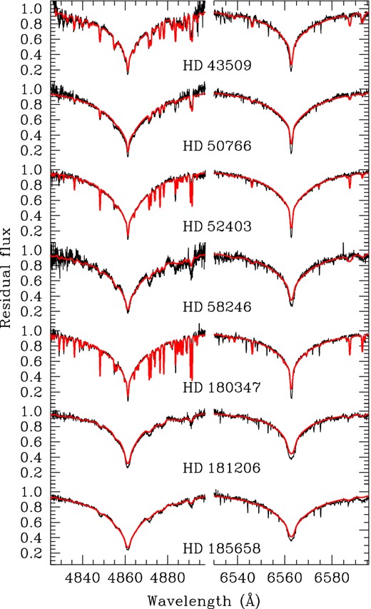
Portions of the spectral echelle orders centred around Hβ and Hα for the programme stars. Overimposed (red lines) are the synthetic spectra computed with the parameters reported in Table 2.
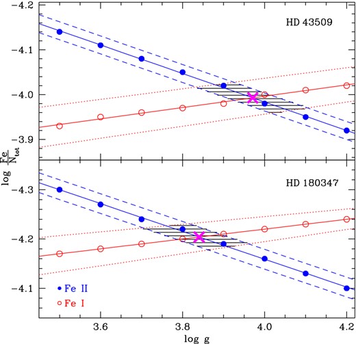
The ionization equilibrium of iron in the atmosphere of HD 43509 anf HD 180347. Open circles indicate abundances of Fe i and filled circles those of Fe ii, both plotted as a function of surface gravity. The dotted (for Fe i) and dashed (for Fe ii) lines are the 1σ bars, while the intersections at log ≈ 3.97 and log ≈ 3.85 are the adopted gravities.
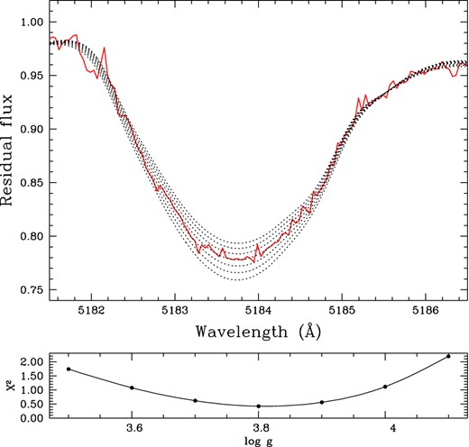
Example of fitting procedure to derive surface gravity for HD 181206 by using Mg i λ 5183 Å. Upper panel: comparison between observed (bold-red line) and synthetic lines (dotted) computed for seven different values of log g, from 3.5 to 4.1 dex (step 0.1 dex), with fixed temperature and abundance. Bottom panel: behaviour of χ2 as a function of log g.
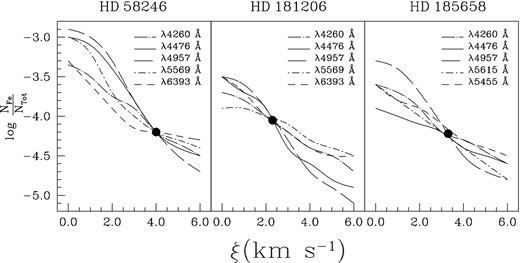
Blackwell diagrams plotted for Fe i lines, left-hand panel refers to HD 58246, central panel to HD 181206 and right-hand panel to HD 185658. The intersections of curves are the adopted microturbulence.
For each element, we calculated the uncertainty in the abundance to be the standard deviation of the mean obtained from individual determinations in each interval of the analysed spectrum. For elements whose lines occurred in one or two intervals only, the error in the abundance was evaluated by varying the effective temperature and gravity within their uncertainties given in Table 2, [Teff ± δTeff] and [log g ± δ log g], and computing the abundance for Teff and log g values in these ranges.
As an example of our spectral synthesis, Fig. 6 shows the fit obtained for our stars in the interval between 5130 and 5250 Å. In that figure stars have been ordered from top to bottom for increasing values of v sin i.
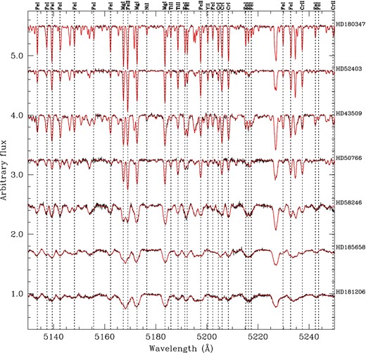
Example of our spectral synthesis in the range 5130–5250 Å. Stars have been ordered from top to bottom by increasing v sin i.
5 INDIVIDUAL STARS
In this section we present the results of the abundance analysis obtained for each star in our sample. The derived abundances and the estimated uncertainties, expressed as |$\log \frac{N_{\rm {el}}}{N_{\rm {Tot}}}$|, are reported in Table 3. The abundance patterns for each star, expressed in terms of solar values (Grevesse et al. 2010), are shown in Fig. 7 .
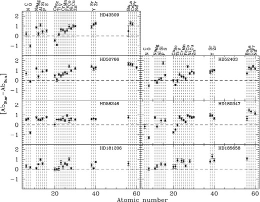
Chemical patterns derived for our targets. Horizontal dashed line corresponds to solar abundance (Grevesse et al. 2010).
Abundances inferred for the Am stars of our sample. Values are expressed in the usual form |$\log \frac{N_{\rm el}}{N_{\rm Tot}}$|. Errors indicated in italic refer to those elements for which spectral lines have been found in one or two intervals only (see text). The abundances reported for oxygen have been evaluated as discussed in Section 6.
| HD43509 | HD50766 | HD52403 | HD58246 | HD180347 | HD181206 | HD185658 | |
|---|---|---|---|---|---|---|---|
| C | −3.41 ± 0.20 | −2.90 ± 0.16 | – | −3.08 ± 0.08 | −3.77 ± 0.19 | −3.28 ± 0.17 | – |
| N | – | – | – | −3.58 ± 0.07 | – | – | – |
| O | −4.35 ± 0.10 | −3.45 ± 0.10 | −3.90 ± 0.10 | −4.15 ± 0.10 | −4.65 ± 0.10 | −3.15 ± 0.10 | −3.30 ± 0.10 |
| Na | −4.92 ± 0.07 | −4.58 ± 0.13 | −5.81 ± 0.01 | −5.08 ± 0.11 | −5.06 ± 0.10 | −5.70 ± 0.08 | −5.71 ± 0.13 |
| Mg | −4.22 ± 0.14 | −4.06 ± 0.14 | −4.63 ± 0.10 | −3.91 ± 0.07 | −4.60 ± 0.14 | −3.94 ± 0.03 | −4.10 ± 0.16 |
| Al | −4.48 ± 0.15 | – | −5.49 ± 0.15 | −5.07 ± 0.09 | – | −4.61 ± 0.15 | – |
| Si | −4.09 ± 0.15 | −3.61 ± 0.15 | −4.36 ± 0.12 | −3.92 ± 0.12 | −4.09 ± 0.16 | −3.97 ± 0.12 | −4.00 ± 0.13 |
| P | – | – | −4.87 ± 0.15 | – | – | – | – |
| S | −4.39 ± 0.12 | −3.92 ± 0.11 | −4.38 ± 0.08 | −4.15 ± 0.07 | −4.46 ± 0.14 | – | −4.42 ± 0.13 |
| Ca | −6.13 ± 0.12 | −5.22 ± 0.15 | −5.73 ± 0.12 | −5.67 ± 0.15 | −6.47 ± 0.07 | −5.70 ± 0.15 | −5.44 ± 0.07 |
| Sc | −9.78 ± 0.07 | −8.82 ± 0.15 | −9.35 ± 0.05 | −8.35 ± 0.10 | −9.37 ± 0.14 | −8.89 ± 0.09 | −8.60 ± 0.10 |
| Ti | −6.92 ± 0.11 | −6.50 ± 0.11 | −7.14 ± 0.12 | −6.55 ± 0.13 | −7.11 ± 0.10 | −7.02 ± 0.18 | −6.18 ± 0.16 |
| V | −7.46 ± 0.13 | −7.64 ± 0.10 | −7.48 ± 0.11 | −7.54 ± 0.10 | −7.31 ± 0.13 | −7.44 ± 0.19 | – |
| Cr | −5.78 ± 0.10 | −5.74 ± 0.13 | −6.00 ± 0.13 | −5.75 ± 0.17 | −5.80 ± 0.12 | −6.14 ± 0.14 | −5.53 ± 0.19 |
| Mn | −6.17 ± 0.15 | −5.82 ± 0.14 | −6.25 ± 0.19 | −6.16 ± 0.09 | −6.14 ± 0.08 | −6.03 ± 0.09 | −5.79 ± 0.18 |
| Fe | −3.94 ± 0.14 | −3.83 ± 0.15 | −4.38 ± 0.16 | −3.60 ± 0.11 | −4.23 ± 0.08 | −4.06 ± 0.08 | −4.20 ± 0.10 |
| Co | −6.00 ± 0.15 | −5.60 ± 0.11 | −5.66 ± 0.09 | −6.61 ± 0.17 | −6.12 ± 0.10 | −6.03 ± 0.12 | – |
| Ni | −5.05 ± 0.12 | −4.82 ± 0.09 | −5.12 ± 0.10 | −5.20 ± 0.15 | −4.99 ± 0.12 | −5.71 ± 0.09 | −5.00 ± 0.15 |
| Cu | −6.83 ± 0.13 | – | −6.93 ± 0.15 | – | −7.10 ± 0.15 | – | – |
| Zn | −6.49 ± 0.05 | −6.25 ± 0.12 | −6.72 ± 0.09 | −6.93 ± 0.12 | −6.70 ± 0.08 | – | – |
| Sr | −8.25 ± 0.13 | −7.74 ± 0.10 | −8.31 ± 0.14 | −8.57 ± 0.06 | −8.19 ± 0.12 | −8.74 ± 0.18 | −8.38 ± 0.13 |
| Y | −8.66 ± 0.12 | −8.65 ± 0.15 | −8.88 ± 0.18 | −9.18 ± 0.14 | −8.89 ± 0.12 | −9.72 ± 0.10 | −8.53 ± 0.18 |
| Zr | −8.18 ± 0.11 | −8.16 ± 0.15 | −8.43 ± 0.07 | −8.89 ± 0.07 | −8.80 ± 0.09 | −8.71 ± 0.06 | −8.56 ± 0.16 |
| Ba | −9.36 ± 0.51 | −8.23 ± 0.14 | −9.16 ± 0.12 | −9.09 ± 0.13 | −9.23 ± 0.19 | −9.27 ± 0.20 | −8.80 ± 0.12 |
| La | −9.64 ± 0.17 | −9.28 ± 0.12 | −9.64 ± 0.15 | – | −9.44 ± 0.11 | – | – |
| Ce | −9.25 ± 0.14 | −8.88 ± 0.13 | −9.29 ± 0.12 | – | −9.12 ± 0.14 | – | – |
| Pr | – | – | −9.89 ± 0.09 | – | – | – | – |
| Nd | – | −9.32 ± 0.12 | −9.44 ± 0.11 | – | −9.44 ± 0.13 | – | – |
5.1 HD 43509
Classified as Am star by Bidelman (1983), this object was never observed at high spectral resolution to date. Our study confirms the Am peculiarity of HD 43509, since we obtained calcium and scandium, respectively, ≈0.5 and ≈1.0 dex under the solar value, and iron-peak elements generally overabundant by 1.0 dex.
5.2 HD 50766
The only previous spectral classification of this star is contained in a paper published in late 70s by Claunsen & Jensen (1979), in which the object is classified as an Am star with spectral peculiarity kA2mA7. No other analysis has been published to date.
Usually Am stars are defined as objects with enhanced iron-peak elements and solar or underabundance of calcium and/or scandium. In our analysis we found overabundance of iron-peak and heavy elements such as strontium, yttrium, zirconium and barium (almost 2 dex larger than the corresponding solar values), while scandium are almost normal in content.
Thus, rather that Am star we can classify this object more properly as a marginal metallic star (Am:).
5.3 HD 52403
This object was also observed by Claunsen & Jensen (1979), who have derived a spectral classification of kA2mA8. A recent spectral classification A1 iii, given by Abt (2004), is in agreement with our results for what concerns the value of log g = 3.5 ± 0.1 dex, corresponding to a moderately evolved star. Our effective temperature is somewhat lower than that corresponding to a spectral type A1 as derived by Abt (2004), but it is in good agreement, at least within the errors, to the determination given by McDonald et al. (2012), who derived Teff = 8216 K by modelling its SED.
Our analysis shows clear evidence that this star could be considered as a marginal Am star. In fact, we derived normal abundance of calcium and light elements, an underabundance of ≈0.5 dex of scandium, while iron-peak and heavy elements show overabundance up to 1 dex.
5.4 HD 58246
HD 58246 is the primary component of a visual double system identified as Am stars by Olsen (1980) and later classified as kA5hF2mF2 by Abt (2008). McDonald et al. (2012) derived Teff = 8323 K by modelling its SED reconstructed by using several literature data; this value is in agreement with the one reported by us in Table 2.
The abundance analysis shows a slight overabundance of metals (≈0.5 dex), while calcium is solar in content. This result is consistent with a classification of marginal Am star.
5.5 HD 180347
This star listed in the Catalogue of Ap, HgMn and Am stars (Renson & Manfroid 2009), is one of the 15 Am stars present in the Kepler field of view. Smalley et al. (2011) observed pulsations in this object with a maximum amplitude less than 0.01 mmag. Later on, McDonald et al. (2012) deriving Teff = 7685 K by modelling its SED, quite in agreement with our result.
Our analysis highlighted a chemical pattern typical of Am stars, with underabundance of calcium (≈0.7 dex) and scandium (≈0.5 dex) and overabundances of iron-peak and heavy elements. Carbon, oxygen, magnesium and titanium display a solar-like abundance, while some light elements like nitrogen, sodium and phosphorus are clearly overabundant. Slight overabundances of silicon and sulphur (≈0.5 dex) have been observed as well.
5.6 HD 181206
Reported as Am star in the Catalogue of Ap, HgMn and Am stars (Renson & Manfroid 2009, spectral type A5 derived from K-line), HD 181206 has been found pulsating in the superWASP survey by Smalley et al. (2011). It is also in the Kepler field of view. Recently this star has been investigated by Tkachenko et al. (2012), who found Teff = 7478 ± 41 K, log g = 3.74 ± 0.18 dex and ξ = 3.55 ± 0.24 km s−1. By using the spectrum synthesis method described in their paper, they also obtained [Fe/H] = −0.30 ± 0.10 dex and a general trend of the chemical pattern under the solar standard composition, with underabundance up to −0.45 dex in the case of titanium. These chemical abundances are then not compatible to those typical of Am stars.
Besides Teff and log g estimated in this work are very close or even consistent (in the case of gravity, within the experimental errors) with those reported by Tkachenko et al. (2012); our results do not support their conclusions about the non-Am nature of HD 181206. In fact, we found slight overabundances (from 0.5 up to 1 dex) of Fe and iron-peak elements, as vanadium, cobalt and nickel, as well as strontium, zirconium and barium. In particular we found [Fe/H] = 0.47 ± 0.10 dex. Our calcium and scandium abundances are instead solar in content.
Given the discrepancy between our results and those obtained by Tkachenko et al. (2012), we tried to derive the iron abundance using an independent method. Elemental abundance of Fe was derived from the measurements of line EWs using the 2013 version of MOOG (Sneden 1973) and assuming LTE conditions. Model atmosphere was computed with atlas9, by using the values of Teff, log g and ξ found by Tkachenko et al. (2012). With these parameters, we obtained [Fe/H] = 0.29 ± 0.17 dex, which is consistent within the errors with the results of our spectral synthesis.
Thus, our results confirm the marginal metallic (Am:) nature of this object, in agreement with what is reported in Renson & Manfroid (2009).
5.7 HD 185658
Reported as Am star in the Catalogue of Ap, HgMn and Am stars (Renson & Manfroid 2009), this star was not detailed studied up to date, at least to our knowledge.
From our work, we can classify this target as a marginal metallic star (Am:), with calcium and scandium solar in content and overabundances of iron-peak and heavy elements.
6 OXYGEN ABUNDANCE
The oxygen abundance, one of the α elements, in the stellar atmospheres is in general an important quantity in the scenario of the Galactic evolution, as well as in the stellar structure and evolution theories. With the exception of the infrared O i λ7771–5 Å triplet, the oxygen lines present in our spectral range are weak and, in the case of rapid rotators, they are blended with other lines or even confused with the continuum. For instance, left-hand side of Fig. 8 shows observed O i λ6155–8 Å triplet (marked with dashed vertical lines) with overimposed the LTE synthetic spectrum computed as described in Section 4. The IR triplet is instead a strong feature easily measured also when high rotational velocity makes difficult the detection of weak lines, see for clarity right-hand side of Fig. 8. Moreover, these lines lie in a clean part of the spectrum (telluric lines are not present) and they do not suffer any kind of blending, nor from atomic or molecular lines. Despite their strength places them in the saturation part of the curve of growth which, however, is not yet completely flat and still provides a sufficient abundance sensitivity for these lines. All these considerations make the O i λ7771–5 Å triplet a good candidate to derive oxygen abundances in our targets. As to Am stars, this triplet has already been used in literature to derive oxygen abundance (see for instance van't Veer-Menneret et al. 1989; Takeda & Sadakane 1997), and the general behaviour is an underabundance with respect to the solar value.
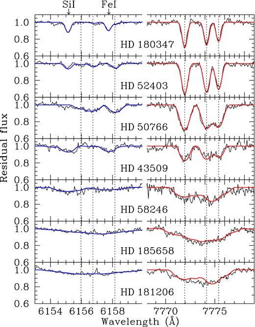
Left-hand side: LTE synthetic spectra computed with atlas9+synthe for O i λ6155–8 Å triplet (blue line) overimposed with the observations (black line). Arrows on top mark the positions of two lines possibly blended with oxygen – Si i λ6155.693 Å and Fe i λ6157.729 Å, respectively. Right-hand side: non-LTE synthetic spectra computed with atlas9+synspec for the O i λ7771–5 Å triplet (red line) overimposed with the observations (black lines). Dashed vertical lines mark the positions of triplets. Stars are ordered from top to bottom for increasing projected rotational velocities.
Previously many authors noticed that this triplet gives systematically higher abundance when compared to those obtained from other lines, in some cases even by one order of magnitude. One reason is that the IR O i lines are formed under conditions far from LTE. In fact, non-LTE spectral synthesis leads to a strengthening of lines and to a decrease in the abundances derived from these lines, as a natural consequence. In the case of A-type main-sequence stars, the usage of non-LTE does not solve the problem, and we still have abundances from λ7771–5 Å triplet higher than those derived from visible lines. This problem has been investigated in the study by Sitnova et al. (2013), who performed non-LTE calculations for this triplet by using model atom by Przybilla et al. (2000), modified according to the calculations of cross-sections for the excitation of O i transitions under collisions with electrons, performed by Barklem (2007). According to their results, they suggested that the introduction of a scaling factor of 1/4 to the rate coefficients for collisions with electrons can reconcile the oxygen abundance derived from different lines.
For the stars of our sample, we explored the possibility of deriving the oxygen abundance by spectral synthesis of the IR triplet at λ7771–5 Å. We also compared the results obtained both with LTE and non-LTE approaches. The LTE analysis has been performed as for the other elements by using atlas9+synthe, while for what concerns non-LTE analysis we used atlas9+synspec (Hubeny & Lanz 2000). synspec reads the same input model atmosphere previously computed using atlas9 and solves the radiative transfer equation, wavelength by wavelength in a specified spectral range. synspec also reads the same Kurucz list of lines we used for the metal abundances. synspec permits to compute the line profiles considering an approximate non-LTE treatment, by means of the second-order escape probability theory (for details see the paper by Hubeny, Harmanec & Stefl 1986).
For each star, the oxygen abundance was calculated by fitting the observed triplet to the synthetic one computed as described before. Model atom has been taken from synspec web site.6 The atomic parameters for the spectral lines were taken from VALD data base (Kupka et al. 1999). The values that best reproduced the observed triplets are reported in Table 3, while the synthetic profiles are shown in Fig. 8. As an additional check, we also compared in Fig. 9, our non-LTE corrections, i.e. Δnon-LTE = log ϵnLTE − log ϵLTE, with the theoretical predictions computed by Sitnova et al. (2013) for various effective temperature, log g = 4.0, solar chemical composition, oxygen abundance fixed to −3.21, and ξ = 2 km s−1. The behaviour of our Δnon-LTE as a function of Teff reflects the one computed by latter authors.

In our sample of stars, oxygen appears to show sub-solar abundances up to ≈1 dex in the case of the two Am stars HD 43509 and HD 180347, moderate underabundances for HD 50766, HD 52403 and HD 58246, while it is solar or slight overabundant for HD 185658 and HD 181201, respectively. This is in agreement with the previous literature results.
7 POSITION IN THE HR DIAGRAM
An accurate location of the Am star in the HR diagram is useful to investigate possible systematic differences in the region occupied by these objects with respect to normal A stars as well as to properly constrain the pulsation instability strip when these stars are pulsating as δ Sct and/or γ Dor variables (see Smalley et al. 2011; Catanzaro & Ripepi 2014).
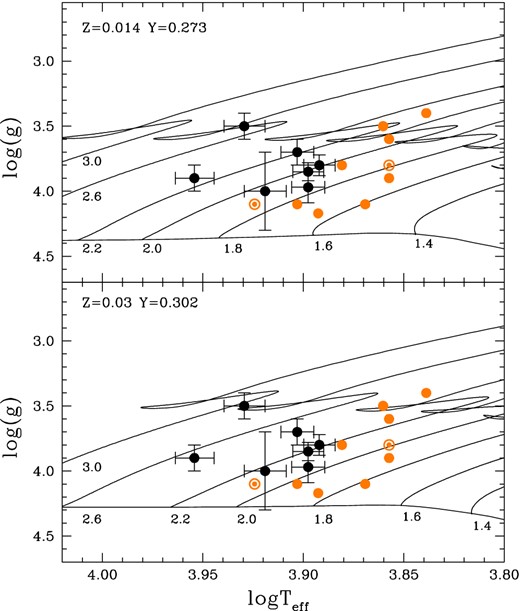
Both top and bottom panels show the log Teff–log g diagram for the seven stars investigated in this paper (black filled circles). Similarly, the light orange symbols (note that filled-open circles show non-Am stars) show the location of the stars studies in our previous works (Balona et al. 2011; Catanzaro et al. 2013; Catanzaro & Ripepi 2014). Top and bottom panels show also the evolutionary tracks (thin solid lines) for the labelled masses as well as the ZAMS from the PARSEC data base for Z = 0.014, Y = 0.273 and Z = 0.03, Y = 0.302, respectively.
Finally, we used the equations (2) and (3) in conjunction with the observed Teff and log g to estimate the log L/L⊙ for the five targets without Hipparcos parallaxes. The result of the whole procedure is shown in Table 1 columns (11) and (12), as well as in Fig. 11, where we added the 11 stars analysed in our previous works on Am stars (Catanzaro et al. 2013; Catanzaro & Ripepi 2014).9 The uncertainties on the luminosities were calculated taking into account both the errors on effective temperature and gravity as well as the rms of each relationship. A comparison of columns (11) and (12) in Table 1 reveals that the use of equations (2) or (3) to estimate the luminosity of the target stars do not produce significant changes.
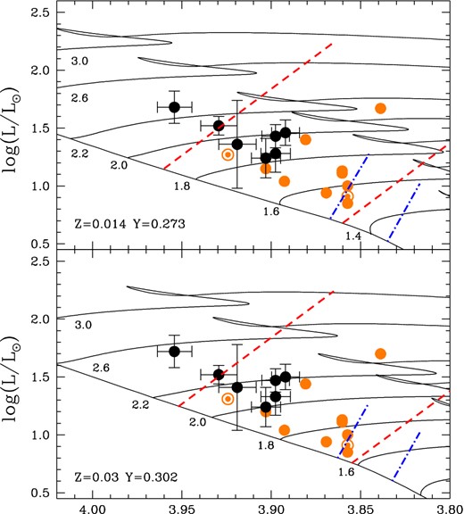
Top and bottom panels show the HR diagram for the seven stars investigated in this paper (black filled circles). Similarly, the light orange symbols (note that filled-open circles show non-Am stars) show the location of the stars studies in our previous works (Balona et al. 2011; Catanzaro et al. 2013; Catanzaro & Ripepi 2014). For comparison purposes we overplot the δ Sct (red dashed lines) and the theoretical edges of the γ Dor (blue dot–dashed lines) instability strips by Breger & Pamyatnykh (1998) and Warner, Kaye & Guzik (2003), respectively. Top and bottom panels show also the evolutionary tracks (thin solid lines) for the labelled masses as well as the ZAMS from the PARSEC data base for Z = 0.014, Y = 0.273 and Z = 0.03, Y = 0.302, respectively.
We also show in Fig. 11 for comparison purposes the edges of the δ Sct (after Breger & Pamyatnykh 1998) and γ Dor (after Warner et al. 2003) instability strips, respectively. In passing, we note that among the seven Am stars presented here, only HD 181206 shows δ Sct pulsations (plus rotational modulation) in the Kepler light curve, whereas HD 180347 and HD 185658 show rotational modulation (see Balona et al. 2015). For the remaining stars there is no information regarding their variability except for HD 43509 that was found constant by Paunzen et al. (2013).
8 DISCUSSION AND CONCLUSIONS
In this work we presented a spectroscopic analysis of a sample of seven stars classified in literature as metallic Am stars. The analysis is based on high resolution spectra obtained at the 91 cm telescope of the Catania Astrophysical Observatory equipped with the new CAOS spectrograph. For each spectra we obtained fundamental parameters such as effective temperatures, gravities, rotational and microturbulent velocities, and we performed a detailed computation of the chemical pattern, as well. To overcome the severe blending of spectral lines, caused by the high rotational velocities of most or our targets, we applied the spectral synthesis method by using synthe (Kurucz & Avrett 1981) and atlas9 (Kurucz 1993a) codes. We used also synspec (Hubeny & Lanz 2000) to compute non-LTE abundances of oxygen from the IR triplet at λ7771–5 Å. With the exception of HD 181206, for which another analysis exists in literature, the other stars were analysed in detail for the first time in this study.
The values of Teff and log g derived here have been used to determine the luminosity of the stars and to place them on the HR diagram.
Our analysis shows that two stars are definitively Am stars, namely HD 43509 and HD 180347, while HD 50766, HD 52403, HD 58246, HD 181206 and HD 185658 are marginal Am stars (Am:). For all the targets, the oxygen abundance has been derived separately by a non-LTE approach, modelling the triplet at λ7771–5 Å. As a general result we found underabundances of oxygen with the exception of HD 185658 (solar) and HD 181206 (+0.2 dex).
The availability of an instrument capable of high-resolution spectroscopy in a wide spectral range such as CAOS will allows us in the future to continue the study of all the Am stars observed by the K2 extension of the Kepler mission that are visible from Catania Astrophysical Observatory and having V ≤ 10 mag. In particular, we will be able to further clean the sample of Am stars observed in the K2 fields from non-Am objects, as well as to fully characterize the spectral properties of the truly Am objects.
The authors wish to thank Dr L. Balona and Dr P. G. Prada Moroni for helpful discussions.
This publication makes use of VOSA, developed under the Spanish Virtual Observatory project supported from the Spanish MICINN through grant AyA2011-24052.
This research has made use of the SIMBAD data base and VizieR catalogue access tool, operated at CDS, Strasbourg, France.
This publication makes use of data products from the Wide-field Infrared Survey Explorer, which is a joint project of the University of California, Los Angeles, and the Jet Propulsion Laboratory/California Institute of Technology, funded by the National Aeronautics and Space Administration.
Atomic data compiled in the DREAM data base (Biemont, Palmeri & Quinet 1999) were extracted via VALD (Kupka et al. 1999, and references therein).
Based on observations made with the Catania Astrophysical Observatory Spectropolarimeter (CAOS) operated by the Catania Astrophysical Observatory.
iraf is distributed by the National Optical Astronomy Observatory, which is operated by the Association of Universities for Research in Astronomy, Inc.
The reader should note that this choice does not affect our determination of Teff and log g since we are reproducing the shape of the SED and not the actual luminosities.
idl (Interactive Data Language) is a registered trademark of Exelis Visual Information Solutions.
[M/H] = log (NM/NH) − log (NM/NH)⊙, where NM and NH are the number of metal and hydrogen atoms per unit of volume, respectively. In turn, [M/H] is related to Z by means of the equation log Z = [M/H]−log Z⊙.
Note that PARSEC models adopt Z⊙ = 0.0152 (for details see section 2.1 in Bressan et al. 2012), but the tracks are available for Z = 0.014.
Note that for homogeneity purposes, equation (2) was used to recalculate the luminosity for stars HD 113878, HD 176843, HD 179458 and HD 187254. As for the remaining seven stars, their luminosities were estimated on the basis of the Hipparcos parallaxes and hence reported here without changes.
