


Abstract
X-ray surface brightness fluctuations in the core of the Perseus Cluster are analysed, using deep observations with the Chandra observatory. The amplitude of gas density fluctuations on different scales is measured in a set of radial annuli. It varies from 7 to 12 per cent on scales of ∼10–30 kpc within radii of 30–220 kpc from the cluster centre. Using a statistical linear relation between the observed amplitude of density fluctuations and predicted velocity, the characteristic velocity of gas motions on each scale is calculated. The typical amplitudes of the velocity outside the central 30 kpc region are 90–140 km s−1 on ∼20–30 kpc scales and 70–100 km s−1 on smaller scales ∼7–10 kpc. The velocity power spectrum (PS) is consistent with cascade of turbulence and its slope is in a broad agreement with the slope for canonical Kolmogorov turbulence. The gas clumping factor estimated from the PS of the density fluctuations is lower than 7–8 per cent for radii ∼30–220 kpc from the centre, leading to a density bias of less than 3–4 per cent in the cluster core. Uncertainties of the analysis are examined and discussed. Future measurements of the gas velocities with the Astro-H, Athena and Smart-X observatories will directly measure the gas density–velocity perturbation relation and further reduce systematic uncertainties in this analysis.
1 INTRODUCTION
The Perseus Cluster is the brightest galaxy cluster in the X-ray sky and has been attracting astronomers attention over the last 40 yr. Being the X-ray brightest cluster, Perseus has led to many fundamental cluster discoveries, such as peaked cluster emission (Fabian et al. 1974), strong Fe xxv and Fe xxvi lines and thermal emission mechanism of the gas (Mitchell et al. 1976), presence of bubbles of relativistic plasma (Boehringer et al. 1993). The cluster was recently observed deeply with the Chandra (see e.g. Fabian et al. 2000, 2011; Schmidt, Fabian & Sanders 2002; Sanders & Fabian 2007, and references therein), XMM–Newton (see e.g. Böhringer et al. 2002; Churazov et al. 2003, 2004; Matsushita et al. 2013, and references therein) and Suzaku (see e.g. Simionescu et al. 2011; Ueda et al. 2013; Werner et al. 2013; Tamura et al. 2014; Urban et al. 2014, and references therein) observatories, as well as by the previous-generation X-ray observatories (see e.g. Forman et al. 1972; Branduardi-Raymont et al. 1981; Mushotzky et al. 1981; Arnaud et al. 1994; Fabian et al. 1994; Furusho et al. 2001; Gastaldello & Molendi 2004). These observations unveiled a variety of structures present in the hot gas of the cluster, reflecting richness and complexity of different physical processes occurring in the intracluster plasma. For example, an east–west asymmetry in the X-ray surface brightness (SB; Schwarz et al. 1992), aligned with a chain of bright galaxies, suggests an ongoing modest merger, which can induce sloshing of the gas and drive gas turbulence (Churazov et al. 2003), while the central few arcmin are dominated by AGN activity in a form of inflated bubbles of relativistic plasma (see e.g. Boehringer et al. 1993; Churazov et al. 2000; Fabian et al. 2000) and weak shocks around them. Rising buoyantly and expanding, the bubbles uplift cooler X-ray gas from the core, producing filamentary structures seen in the optical, far-ultraviolet and soft X-ray, and excite internal waves, energy of which is transported to gas turbulence (Balbus & Soker 1990; Churazov et al. 2001; Omma et al. 2004; Forman et al. 2007; Fabian et al. 2008; Canning et al. 2014; Hillel & Soker 2014).
The truly spectacular statistics accumulated by the Chandra observations of Perseus (over 85 million counts within 6 arcmin from the centre, with 100s and 1000s counts per sq. arcsec) makes this data set an extremely powerful tool to probe structures in the intracluster medium (ICM) on a range of spatial scales. Carefully modelling the Poisson noise, one can probe small-scale fluctuations, which we cannot see in the cluster images by visual inspection. Here, we present statistical analysis of these SB and density fluctuations, using the power spectrum (PS) statistics. We will examine the radial variations of the PS within the Perseus core (220 × 220 kpc), while its energy dependence will be considered in our future works.
Statistical analysis of the X-ray SB and/or density, pressure fluctuations was done for two clusters so far: the Coma Cluster (Schuecker et al. 2004; Churazov et al. 2012) and AWM7 (Sanders & Fabian 2012). It was shown, for example, that the amplitude of density fluctuations in Coma ranges from 5 to 10 per cent on scales 30–500 kpc, leading to non-trivial constraints on perturbations of the cluster gravitational potential, turbulence, entropy variations and metallicity. The fluctuations appear to be correlated, implying suppression of strong isotropic turbulence and conduction (Sanders et al. 2013).
The Chandra data on Perseus allow us to probe fluctuations on similar or even smaller scales, down to few kpc. The main questions we address here include: what is the amplitude of density fluctuations and how does it vary with the distance from the cluster centre (Section 5.1); what is the PS of gas turbulent motions (Section 5.2); how clumpy is the gas in the core (Section 5.3). To answer these questions, various instrumental effects [e.g. point spread function (PSF) variations, detector quantum efficiency fluctuations], contribution of the unresolved point sources, subtraction of the Poisson noise as well as its fluctuations need to be treated carefully. We extensively investigate various systematic uncertainties of the analysis and discuss them in Section 6.
This paper is complementing our series of publications on SB and density fluctuations in the core of the Perseus Cluster. One application of the velocities of gas motions measured here is discussed in Zhuravleva et al. (2014a). There we show that turbulent dissipation in the cluster core produces enough heat to balance locally radiative energy losses from the ICM at each radius. Therefore, turbulence may play an important role in AGN feedback loop and be the key element in resolving the gas cooling flow problem (Zhuravleva et al. 2014a). In our next paper, we will discuss the nature of the fluctuations by measuring cross-spectra of fluctuations in different energy bands (Zhuravleva et al., in preparation). Similar analysis for the Virgo and Coma clusters are in progress.
Throughout the paper, we adopt Λ cold dark matter cosmology with Ωm = 0.3, ΩΛ = 0.7 and h = 0.72. At the redshift of Perseus, z = 0.01755, the corresponding angular diameter distance is 71.5 Mpc and 1 arcmin corresponds to a physical scale 20.81 kpc. Position of the cluster centre is taken from the NASA/IPAC Extragalactic Database1 and corresponds to the position of the central galaxy NGC1275. The total galactic H i column density2 is 1.36×1021 cm−2. Solar abundances of heavy elements are taken from Anders & Grevesse (1989). We define the characteristic scale-dependent amplitude A3D(k) through the PS P3D(k) as follows |$A^2_{{\rm 3D}}(k)=\int 4\pi P_{{\rm 3D}}(k)k^2\mathrm{d}k=4\pi P_{{\rm 3D}}(k) k^3$|. A wavenumber k is related to a spatial scale l without a factor 2π, i.e. k = 1/l.
2 INITIAL DATA PROCESSING
For our analysis we use public Chandra data with the following ObsIDs: 3209, 4289, 4946, 4947, 4948, 4949, 4950, 4951, 4952, 4953, 6139, 6145, 6146, 11713, 11714, 11715, 11716, 12025, 12033, 12036, 12037. The initial data processing is done using the latest calibration data and following the standard procedure described in Vikhlinin et al. (2005). For the analysis, we choose 0.5–3.5 keV energy band. In this band, the gas emissivity has a weak temperature dependence (within a range of temperature variations present in the Perseus core) as shown in Fig. 1 , and, therefore, the uncertainty associated with the conversion of PS of SB fluctuations to the PS of density fluctuations is reduced (see Section 5.1).
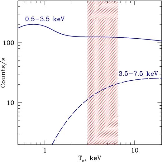
Emissivity of an optically thin plasma as a function of temperature observed by the ACIS-I detector on Chandra in two energy bands: 0.5–3.5 (filled) and 3.5–7.5 (dashed) keV. Abundance of heavy elements is assumed 0.5 relative to solar. Shaded region shows a range of gas temperatures in the core of the Perseus Cluster (3–6.5 keV). Notice, that for the 0.5–3.5 keV band, the emissivity is almost independent of the temperature within this region. Therefore, the X-ray surface brightness in this shaded band IX is just a function of gas electron number density ne, namely, |$I_{\rm X}\sim \int n_{\rm e}^2 \mathrm{d}l$|, where l is the length of the line of sight.
Correcting for the exposure, vignetting effect and subtracting the background, a mosaic image of the Perseus Cluster is produced, which is shown in Fig. 2. The combined exposure map is shown in Fig. 3. The total exposure of the cleaned data set is ∼1.4 Ms. Notice, that the exposure coverage is inhomogeneous. It varies from few × 106 s in the centre down to few × 105 s in some distal regions. The uncertainties associated with such inhomogeneous coverage are discussed in Section 6.
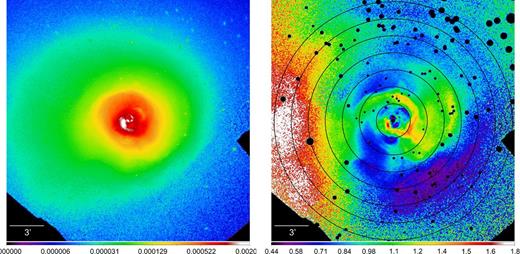
Left: Chandra mosaic image of the Perseus Cluster in the 0.5–3.5 keV band. The units are counts s −1pixel−1. The size of each pixel is 1 arcsec. Right: residual image of the cluster (the initial image divided by the best-fitting spherically symmetric β-model of the surface brightness), which emphasizes the surface brightness fluctuations present in the cluster. Point sources are excised from the image. Black circles show the set of annuli used in the analysis of the fluctuations. The width of each annulus is 1.5 arcmin (≈30 kpc). The outermost boundary is at a distance 10.5 arcmin (≈220 kpc) from the centre. For display purposes, both images are lightly smoothed with a 3 arcsec Gaussian.
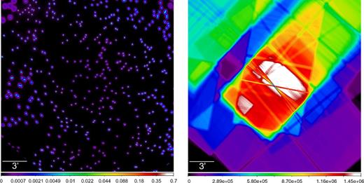
Left: simulated map of the combined Chandra PSF within the mosaic image of the Perseus Cluster. The random positions of individual PSFs are used (see Section 2 for details). Right: the combined exposure map in seconds (lightly smoothed with a 3 arcsec Gaussian for display purposes).
The Perseus data set includes observations with different offsets. For the analysis of SB fluctuations, it is essential to know the PSF at each point within the cluster image. We randomly generate positions, where the PSF is checked. The PSF at each position for each observation is determined from the Chandra PSF libraries (Karovska et al. 2001). By combining the PSF model images with weights proportional to exposure of each observation, the final PSF map is obtained. These maps are used to correct the PS of the SB fluctuations (Section 4). In order to illustrate the variations of the PSF shape within the cluster mosaic image, we show the PSF map divided by the exposure map in Fig. 3. Notice a non-monotonic behaviour of the PSF and its elongated (distorted) shape close to the edges of the image.
3 SPHERICALLY SYMMETRIC MODEL
The spherically symmetric radial SB profile of the Perseus is shown in Fig. 4. Fitting this profile with a β-model assuming photon counting noise only, gives the core radius rc = 1.26 arcmin and the slope of the model β = 0.53 with negligible uncertainties. Allowing for 10 per cent systematic error on the SB in each annulus, the uncertainties become 0.1 and 0.01 for rc and β, respectively. Throughout the paper, this model is used as a default model of the unperturbed cluster. Sensitivity of our results to the choice of the model are discussed in Section 6.
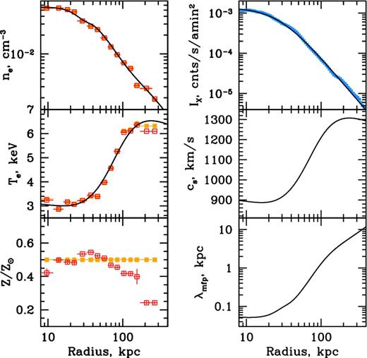
Radial profiles of thermodynamic properties of the Perseus Cluster obtained from Chandra observations in the 0.6–9 keV band. Orange (filled) and red (open) points with 1σ error bars on the left panels show the deprojected gas number electron density ne, electron temperature Te and abundance of heavy elements relative to solar Z/Z⊙, assuming the latter one is constant 0.5 relative to solar or is a free parameter in the fitting spectral model of an optically thin plasma, respectively. Analytic approximations of the observed profiles by smooth functions are shown with black filled curves. Blue points on the top right panel show the spherically symmetric X-ray surface brightness profile obtained from the 0.5–3.5 keV image, while the black curve shows its best-fitting β-model with the core radius rc = 1.26 arcmin and the slope β = 0.53. The cluster sound speed cs and the mean free path λmfp calculated from the approximations are shown in the middle and bottom panels on the right.
4 POWER SPECTRUM OF THE SURFACE BRIGHTNESS FLUCTUATIONS
X-ray SB of galaxy clusters is typically peaked towards centres and decreases rapidly with radius. This is especially true for relatively dynamically relaxed clusters like Perseus (Mantz et al. 2014). Therefore, the PS of the initial SB will be dominated by this gradient, leading to a large power on small wavenumbers k and contamination of the power on larger k. In order to avoid this, we first remove the global SB gradient and analyse fluctuating part of the SB only. One way of doing it is to subtract the model of the cluster. However in this case additional weights proportional to the global SB profile have to be introduced in order to treat the fluctuations at different radii equally. Instead, in order to work with dimensionless units of the SB fluctuations, we divide the image of the Perseus Cluster by a simple spherically symmetric β-model of the SB (the choice of the model is arguable and is discussed in Section 6). Fig. 2 shows the residual image of the SB fluctuations in Perseus. Notice a variety of structures of different sizes and morphologies present in the cluster, especially within the central 3 arcmin. Let us quantify these structures statistically, by measuring their power as a function of length-scale.
We use a modified Δ-variance method (Arévalo et al. 2012) to calculate the PS of SB fluctuations. This method is tuned to cope with non-periodic data with gaps, the PS of which are smooth functions. Dashed curves in Fig. 5 show the PS of SB fluctuations in the central 3 arcmin (central AGN is excluded) and in a broad annulus 3–10.5 arcmin. The spectra decrease with wavenumber k and reach constant value on small scales, where the signal is dominated by the Poisson noise.
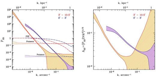
Left: power spectra (PSs) of the X-ray surface brightness (SB) fluctuations in the Perseus Cluster in the central 3 arcmin (purple) and in the annulus 3–10.5 arcmin (orange). Dash curves: the initial PS. Dotted regions: PS of the Poisson noise. Dash–dotted curves: PS of the combined Chandra PSF in both analysed regions. Hatched region with filled boundaries: PS of the SB fluctuations after subtraction of the Poisson noise. Both statistical (1σ) and stochastic uncertainties are taken into account. Notice, that very high statistics of counts accumulated by the 1.4 Ms observations allows us to probe fluctuations on a broad range of length-scales, from >100 kpc down to few kpc (comparable with the mean free path). Right: amplitude of the SB fluctuations in the same regions, obtained from the PS corrected for the PSF (see Section 4). Notice, that the amplitude of fluctuations varies with the radius. For these two regions a maximal difference by a factor of 4 is reached on ∼17 kpc scale.
Finally, the PS of SB fluctuations have to be corrected for the Chandra PSF and for the contribution of the unresolved point sources on small scales. Performing multiple realizations of the PSF maps (see Section 2), and each time calculating the PS of the map within the region of our interest, the mean spectrum of the PSF is obtained. Dash–dotted curves in Fig. 5 show the PSF PS in central 3 arcmin and in the annulus 3–10.5 arcmin. The deviations of the PSF shape from a δ-function are reflected in a drop of power on the high-k end of the spectrum. Dividing the PS of the SB fluctuations by the PSF PS, the SB power suppressed by the PSF is recovered.
The contribution of unresolved point sources is estimated by using the Perseus sensitivity map and by obtaining the shape and normalization of the log N–log S distribution of the resolved sources. In case of the Perseus Cluster, the contribution of the unresolved sources is negligible (within the cluster core).
After applying all corrections described above, the characteristic amplitude A2D(k) of the SB fluctuations is calculated, namely |$A_{{\rm 2D}}(k)=\sqrt{P_{{\rm 2D}}(k)2\pi k^2}$|, where P2D(k) is the measured PS. The amplitude is a more convenient characteristic since its units are the same of the variable in a real space. Fig. 5 shows the amplitude of SB fluctuations in the central 3 arcmin region and in the outer annulus 3–10.5 arcmin. High statistics of counts allows us to probe the SB fluctuations on a broad range of length-scales – more than an order of magnitude, down to the scales comparable with the mean free path (see Fig. 4). The amplitude varies from ∼3–14 per cent on scales 2–50 kpc in the central 3 arcmin to ∼2–33 per cent on scales ∼14–170 kpc in the 3–10.5 arcmin region. The fact that the amplitudes in both regions differ at least by a factor of 3 over a broad range of scales shows that the amplitude of SB fluctuations in Perseus varies with radius. Therefore, instead of global characterization of the fluctuations in the cluster core, we consider below the fluctuations in a set of narrow radial annuli.
5 RESULTS
5.1 Power spectrum of density fluctuations
We divided the cluster into a set of radial annuli with a width 1.5 arcmin (≈30 kpc; Fig. 2) and calculated the PS of SB fluctuations in each annulus, subtracting the Poisson noise and correcting for the unresolved point sources and the PSF. The latter one was done using PSF PS shown in Fig. 6.
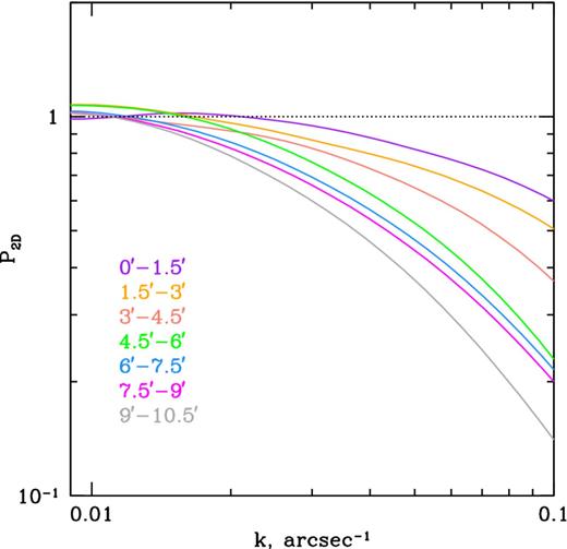
Power spectrum (PS) of the combined Chandra PSF obtained in each annulus of the Perseus Cluster in our analysis (Fig. 2). The combined PSF accounts for the shape of the PSF at different offsets and exposure of each observation (see Section 2). Each spectrum is averaged over 10 spectra of different realizations of the PSF map. Since the PSF is not a δ-function, the PS deviate significantly from unity (dotted line), especially on scales smaller than 15 kpc (k ≈ 0.02 arcsec−1).
We tested this procedure using high-resolution cosmological simulations of galaxy clusters (Nagai, Vikhlinin & Kravtsov 2007; Nelson et al. 2014). Using non-radiative simulations, we obtained the PS of density fluctuations directly from the simulated 3D data for a sample of six relatively relaxed clusters and recovered the PS from projected images of the X-ray SB (applying the same procedure we use for the observed X-ray images). The details of the sample and the analysis are described in Zhuravleva et al. (2014b). Direct comparison of both PS (or amplitudes) confirms that the X-ray images can provide reasonably accurate measurements of the PS of density fluctuations. Fig. 7 shows an example of one of the clusters in our sample.
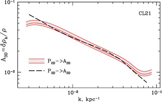
Amplitude of density fluctuations in the inner 200 kpc (radius) region in the simulated relaxed galaxy cluster (CL21 cluster with total mass M500c = 6.08 × 10¹⁴M⊙ at r500c = 1215.2 kpc; see Zhuravleva et al. (2014b) for details) obtained from the 3D density information (dash black curve) and recovered from the image of the X-ray surface brightness (hatched orange/red region). The width of the hatched region reflects the uncertainty of the recovered 3D amplitude of density fluctuations due to variations of the converting geometrical factor with the projected radius. Notice that the true (from the 3D data) amplitude of density fluctuations is within the hatched region. This confirms that the observational procedure of measuring the amplitude of density fluctuations from the X-ray images recovers reasonably accurate the amplitude of the 3D density fluctuations.
The accuracy of the recovery of the 3D spectrum in each annulus depends on how steep the emissivity profile is. In case of the Perseus Cluster, the emissivity is strongly peaked towards the centre, therefore the conversion factor significantly varies within the radial annuli. The narrower the annulus, the smaller the uncertainty. To do the conversion, we use the mean (within the annulus) value of this factor. In Section 6, we will discuss the uncertainties associated with this step of the analysis.
Fig. 8 shows the amplitude of density fluctuations A3D obtained in each annulus from the PS of SB fluctuations P2D as a function of wavenumber k. Scales, which are smaller than the width of each annulus (≈30 kpc) are plotted. Hatched regions show the amplitude on wavenumbers, over which we deem the measurements are least affected by the uncertainties and more robust against the observational limitations. The choice of the high-k limit is set by the statistical uncertainty or by the PSF distortions of the amplitude. For both cases, the uncertainty is less than 20 per cent in this hatched region. At low k, we exclude scales, on which the amplitude flattens or decreases towards smaller k. This flattening is most likely determined by the presence of several characteristic length-scales (e.g. distance from the centre, scale heights, additional driver of fluctuations) and by the uncertainties in the choice of the underlying cluster model (see Section 6).
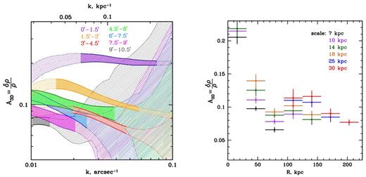
Left: amplitude of density fluctuations in the Perseus Cluster versus wavenumber calculated in a set of radial annuli shown in Fig. 2. Hatched regions show the amplitude on scales where the measurements are least affected by systematic and statistical uncertainties. The width of each curve reflects estimated 1σ statistical and stochastic uncertainties. Right: radial profiles of the amplitude of density fluctuations measured on certain scales (see the legend). Notice, that the amplitude decreases with the radius and increases with the length-scale of fluctuations.
The amplitude of density fluctuations is less than 15 per cent, except for the central ∼30 kpc. Table 1 summarizes the characteristic values of the amplitude in all considered regions. The amplitude in the innermost region is noticeably higher and the curve itself is flatter than in other regions. This is not surprising, since a significant fraction of the volume of this region is dominated by sharp edges around bubbles of relativistic plasma, shocks around them, filamentary structures and absorption features, flattening the high-k end of the amplitude. Simple tests showed the drop of power on small scales when these features are excluded from the analysis. The radial variations of the amplitude at different scales is shown in the right panel of Fig. 8. Notice, that the amplitude decreases with the distance from the centre and it increases with the scale (characteristic size) of the fluctuations.
| Annulus | Amplitude of density fluctuations | Amplitude of one-component velocity | ||||
|---|---|---|---|---|---|---|
| A3D = δρ/ρ | V1, k, km s−1 | |||||
| l = 10 kpc | l = 20 kpc | l = 30 kpc | l = 10 kpc | l = 20 kpc | l = 30 kpc | |
| 0–1.5 arcmin (0–31 kpc) | 0.22 | – | – | 200 | – | – |
| 1.5–3 arcmin (31 - 62 kpc) | 0.11 | 0.14 | – | 110 | 140 | – |
| 3–4.5 arcmin (62–94 kpc) | 0.08 | – | – | 90 | – | – |
| 4.5–6 arcmin (94–125 kpc) | 0.09 | 0.1 | 0.11 | 110 | 130 | 140 |
| 6–7.5 arcmin (125–156 kpc) | – | 0.09 | 0.12 | – | 120 | 150 |
| 7.5–9 arcmin (156–187 kpc) | – | 0.08 | 0.09 | – | 100 | 120 |
| 9–10.5 arcmin (187–219 kpc) | – | – | 0.08 | – | – | 100 |
5.2 Velocity power spectrum
Fig. 9 shows the amplitude of one-component velocity versus wavenumber obtained from the relation (7) in all seven radial annuli in the Perseus core, as well as the radial profiles of the amplitude on certain scales. Like in Fig. 8, hatched regions show the amplitude on scales, where the measurements are least affected by systematic and statistical uncertainties. Notice that the velocity amplitude is higher towards the centre, suggesting a power injection from the centre. The spectra (amplitudes) show similar dependence on k, larger fluctuations are on larger k, consistent with cascade turbulence. The slope of the velocity PS is broadly consistent with the slope for canonical Kolmogorov turbulence, accounting for the errors and uncertainties. Within the ‘robust’ range of scales, V1, k varies from ∼70 up to ∼210 km s−1 on scales ∼5–30 kpc (see Table 1). The velocity amplitudes quantitatively match our expectations of typical velocities in the ICM from various observational constraints (see e.g. Churazov et al. 2004; Schuecker et al. 2004; Werner et al. 2009; Sanders et al. 2010; Sanders, Fabian & Smith 2011; de Plaa et al. 2012; Sanders et al. 2013; Pinto et al. 2015, and references therein) and numerical simulations (see e.g. Norman & Bryan 1999; Dolag et al. 2005; Iapichino & Niemeyer 2008; Lau, Kravtsov & Nagai 2009; Vazza et al. 2011; Miniati 2014, and references therein). Future direct measurements of the velocity of gas motions with X-ray calorimeter on-board Astro-H observatory (Takahashi et al. 2014) will allow us to test the density–velocity relation (7). Recently proposed observational strategy for the Perseus Cluster maps the cluster core in radial and azimuthal directions, enabling us to do the calibration (Kitayama et al. 2014).
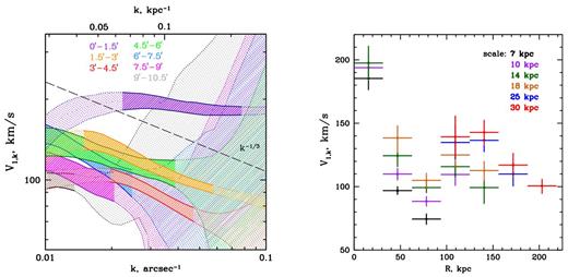
Left: amplitude of one-component velocity of gas motions versus wavenumber k = 1/l, measured in a set of radial annuli (see the legend) in the Perseus Cluster. The velocity at each scale is obtained from the amplitude of density fluctuations, shown in Fig. 8, using relation (7). The colour coding and notations are the same as in Fig. 8. The slope of the amplitude for pure Kolmogorov turbulence (Kolmogorov 1941), k−1/3, is shown with dash line. Right: radial profiles of one-component velocity amplitude measured on certain length-scales written in the legend.
Fig. 10 shows the radial profile of the Ozmidov scale lO and a range of scales we are probing in each annulus (hatched regions in Fig. 9). One can see that lO is within the interval of scales we are probing at each distance from the centre within the cluster core. This means that the main assumption behind the derivation in Zhuravleva et al. (2014b) is satisfied, namely the Ozmidov scale is smaller than the injection scale of turbulence (assuming that we are probing velocity PS within the inertial range). Notice, that we do not show lO at R < 20 kpc since the measured gas entropy is flat towards the centre, leading to lO → ∞.
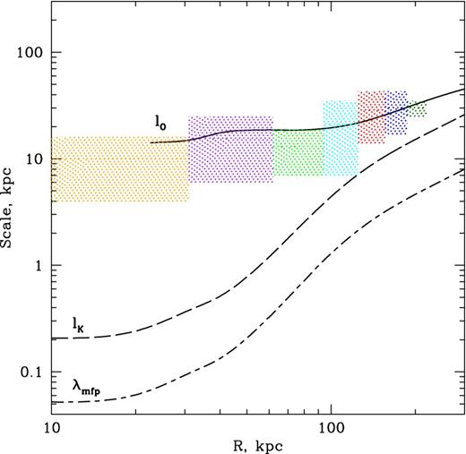
Characteristic length-scales present in the Perseus Cluster at different distances R from the centre. Coloured shaded regions: range of scales, on which our measurements are least affected by systematic and statistical uncertainties (hatched regions in Figs 8 and 9). Filled curve: the Ozmidov scale lO of turbulence in the core of Perseus, obtained assuming local balance between turbulent heating and radiative cooling (relation 8). We do not plot lO in central ∼20 kpc, since the measured gas entropy is flat there, leading to lO → ∞. Dash curve: the Kolmogorov (dissipation) scale lK for unmagnetized plasma (relation 9). Dot–dashed curve: the electron mean free path for unmagnetized plasma. See Section 5.2 for discussion.
We cannot claim, of course, that the structures in the SB are due to turbulence only. For example, there are many bubbles of relativistic plasma in the Perseus core (see e.g. Boehringer et al. 1993; Churazov et al. 2000; Fabian et al. 2000), which may contribute to the signal. The question is whether their contribution is dominant in the considered regions. Various sharp structures (e.g. bubble edges) would give the slope of the amplitude k−1/2, which is hard to discriminate from the Kolmogorov slope k−1/3 accounting for the uncertainties of our measurements and the assumptions used. However the contribution of the bubbles to the signal can be easily seen if we repeat the analysis excluding the known bubbles from the image of Perseus. Fig. 11 shows the one-component velocity amplitude calculated from such image. Notice, that the velocity amplitude decreases by a factor ∼1.6–1.2 depending on scale in the central 1.5 arcmin. This is expected since bubbles in this region are particularly prominent and occupy a substantial fraction of the volume. In the 1.5–3 arcmin annulus, this factor is ∼1.15 over the whole range of scales. Outside 3 arcmin, the exclusion of bubbles from the analysis does not change the measured velocity amplitude.

Left: residual image of the Perseus Cluster in the 0.5–3.5 keV band (the same as Fig. 2) with excluded bubbles of relativistic plasma taken from Fabian et al. (2011) (black ovals). Right: one-component velocity amplitude versus wavenumber obtained from the image on the left. The colour-coding and labels are the same as in Fig. 9.
Sound waves (Fabian et al. 2006; Sternberg & Soker 2009), mergers and gas sloshing (Markevitch & Vikhlinin 2007) might also contribute to the observed spectrum of the density fluctuations. Unsharp masking of the Perseus Cluster revealed quasi-spherical structures (‘ripples’) in the SB, which have been interpreted as isothermal sound waves (Fabian et al. 2000, 2003). An alternative interpretation is stratified turbulence, which arises naturally in the cluster atmosphere, where rough estimates give Froude number Fr ∼ 0.3–1 (Zhuravleva et al. 2014b). In this case, the radial size of each ‘ripple’ Δr is determined by HV/cs, where H is the characteristic scale height and V is the velocity amplitude. For example, in the 1.5–3 arcmin annulus in Perseus, the scale height H is ∼40–70 kpc, the sound speed cs ∼ 900 km s−1 and the velocity measured from the SB fluctuations is ∼100–140 km s−1. This gives us typical radial sizes of the fluctuations ∼5–10 kpc, which are consistent with those seen in the X-ray image of the cluster once the large-scale asymmetry in SB is removed. Certainly, we cannot claim that the observed fluctuations are associated with the stratified turbulence only. The question on the nature of the fluctuations will be addressed in our future work. At the very least, the measured turbulent velocities can be treated as an upper limit.
5.3 Gas clumping
Gas clumping leads to an overestimate of the gas density and, as a consequence, affects the gas mass and total hydrostatic mass measurements of galaxy clusters (see e.g. Lau et al. 2009) as well as the Sunyaev-Zeldovich measurements of the Compton parameter (e.g. Khedekar et al. 2013). Numerical simulations predict clumping <1.05 in central 0.5r500, ∼1.1–1.4 at r500 and up to 2 at r200 (see e.g. Mathiesen, Evrard & Mohr 1999; Nagai & Lau 2011; Roncarelli et al. 2013; Zhuravleva et al. 2013; Vazza et al. 2013). The clumping factor obtained from X-ray observations of cluster outskirts is slightly higher and varies from ∼2 to ∼3 at r200 (see e.g. Urban et al. 2014; Walker et al. 2012; Morandi & Cui 2014, and references therein). The main challenges of the clumping measurements from the X-ray observations are a very low X-ray SB in cluster outskirts, where clumping is expected to be higher, and, in contrast, a low value of the clumping factor, less than 5 per cent according to numerical simulations, in the bright cluster cores.
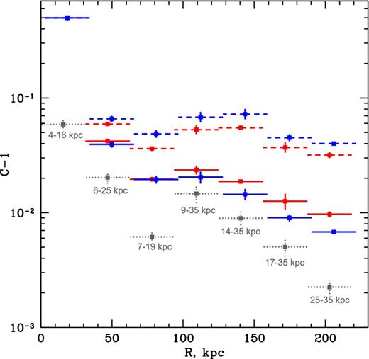
Radial profile of the clumping factor C − 1 in the core of the Perseus Cluster obtained from the relation (11) using the measurements of density fluctuations power spectra. Red points: the measured density spectrum is fitted by a power-law function with the Kolmogorov slope −11/3 and extended to small and large scales, which we do not probe in our analysis. Blue points: the slope of the power-law function is assumed −3.1 and −4 for the innermost annulus 0–1.5 and for other six regions, respectively. The slope −4 is obtained from the power spectrum of density fluctuations in the broad annulus 1.5–10.5 arcmin. Dash points: kmin = 1/R, kmax = ∞. Filled points: kmin = 0.01 arcmin−1 (inverse width of each annulus), kmax = ∞. Grey dotted points: clumping factor obtained from the measured power spectrum of density fluctuation directly, avoiding any approximations with the power laws. Measurements within the range of scales least affected by the uncertainties (hatched regions in Fig. 8) are used. The corresponding scales are written below each point. Notice, that the clumping factor is less than 7–8 per cent outside the central ∼30 kpc.
6 UNCERTAINTIES IN THE ANALYSIS
In this section, we examine various systematic uncertainties in the analysis. Namely, we consider uncertainties associated with (i) the choice of the unperturbed cluster density model; (ii) the bias of the Δ-variance method used for the PS calculations; (iii) inhomogeneous exposure coverage; (iv) conversion P2D to P3D; (v) velocity measurements.
Even though the list of uncertainties is, admittedly, long, a conservative estimate of the total uncertainty on the amplitude of density fluctuations (one-component velocity) is less than 50 (60) per cent.
6.1 Underlying model of the surface brightness
Decomposition of the cluster image into ‘perturbed’ and ‘unperturbed’ components is ambiguous. Physically motivated, the underlying model of the ‘unperturbed’ component should reflect the global potential of the cluster in equilibrium, i.e. when the isosurfaces of the gas density and temperature are aligned with the equipotential surfaces. Our default choice of the model – β-model for the azimuthally averaged SB (or just mean SB) – seems to be a reasonable choice of such ‘unperturbed’ model at least for (or close to) relaxed galaxy clusters. However, one can see the large-scale, west–east asymmetry in the SB of the Perseus Cluster (Fig. 2, left), which might question our most simple and conservative choice. To check how the global cluster asymmetry affects the density amplitude measurements, we repeated the analysis, using two other β-models of the SB averaged in 180° sectors. The best-fitting parameters of the β-model in the east (90°÷270°) and the west (−90°÷90°) sectors are rc = 1.76 and 0.89 arcmin, β = 0.61 and 0.48, respectively. Choosing these underlying models, the maximal deviations of the density amplitude from the default case are on the largest scales in each annulus (typically ∼30–20 kpc) and are less than 10 per cent in the central 6 arcmin, less than 17 per cent in the 6–7.5 arcmin annulus and less than 30 per cent at the distance 7.5–10.5 arcmin from the cluster centre (see Table 2).
Going beyond this simple spherically symmetric model implies that we believe that the underlying cluster potential is more intricate. It is not clear to what degree of complexity of the model we should go. There is always a danger that some of the structures unrelated to the cluster gravitational potential are removed. We made a number of tests, introducing more flexibility to the β-model, by patching it on large scales to account for possible complexity of the potential. Namely, our patched model is defined as Ipm = IβSσ[IX/Iβ], where Iβ is the β-model of azimuthally averaged SB, Sσ[ · ] denotes Gaussian smoothing with the smoothing window size σ and IX is the clusters X-ray SB. Varying the size of the smoothing window, the model changes from most conservative symmetrical β-model (large σ) to most complicated (and clearly implausible) one, which accounts for structures on all scales (small σ).4 Examples of such models and the corresponding residual images of the SB fluctuations are shown in Fig. 13. Models with large σ (e.g. ∼80 arcsec) remove the large-scale (east–west) asymmetry of the cluster, while those with a smaller σ absorb more features of the image on smaller scales. Fig. 14 shows the amplitude of density fluctuations in 3–4.5 arcmin annulus measured from the residual images in Fig. 13. Notice, that the removal of the large-scale asymmetry (blue hatched region) does not change the amplitude of density fluctuations relative to spherically symmetric β-model (red hatched region) over the range of scales probed in our analysis (<30 kpc). As expected, the more complex models (with the smaller σ), the broader range of scales, on which the amplitude is suppressed, and the stronger the suppression of the amplitude on the largest scales.
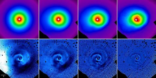
Top: underlying models of ‘unperturbed’ surface brightness in the Perseus Cluster. From left to right: spherically symmetrical β-model (default choice), patched β-models with σ = 80 arcsec (removes large-scale asymmetry), σ = 30 arcsec and σ = 10 arcsec (see Section 6.1 for the details). Bottom: residual images of the SB fluctuations in Perseus obtained from the initial image divided by the underlying model (top panels). The smaller the σ the smaller the structures included to the model and the less structures remain in the residual image.
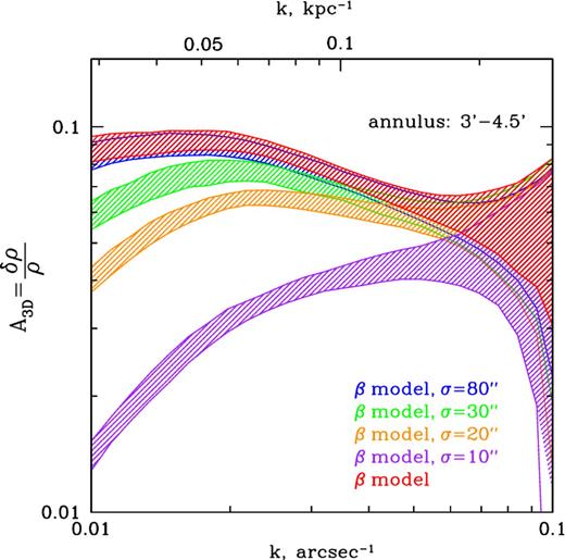
Amplitude of density fluctuations in the 3–4.5 arcmin annulus in the Perseus Cluster obtained by using spherically symmetrical β-model as the underlying one (red) and more flexible models shown in Fig. 13. Notice, that the removal of the global cluster asymmetry (blue hatched region) does not affect the amplitude measurements relative to the default model (red) on scales we are probing. Also, notice that even if the amplitude suppression is present on scales, which are included to the underlying model (as expected), the amplitude on smaller scales, which are not affected by the model, remains almost the same. This means that the measured amplitude is indeed due to the presence of fluctuations of these scales and not due to the power leakage from the large scales.
6.2 Bias in the Δ-variance method
The normalization of the PS obtained through the Δ-variance method may be biased slightly, depending on the slope of the PS (see appendix B in Arévalo et al. 2012). The approximations of the initial PS of SB fluctuations with a power-law functions give the slopes ∼− 3to − 3.8 depending on the distance from the cluster centre. Therefore, the normalization of the measured amplitude of density fluctuations is on average overestimated by ∼20–30 per cent and slightly lower, by <10 per cent, in the outermost (7.5–10.5 arcmin) annuli, see Table 2.
6.3 Inhomogeneous exposure coverage
The exposure map is not uniform and the brightness of the cluster itself varies across each annulus as seen in Figs 2 and 3. Both arguments may bias the measured amplitude of density fluctuations. By default, when calculating the amplitude by taking RMS of fluctuations present in filtered images, we use most uniform weighting scheme, w = 1, i.e. we treat all pixels in the image with the same weight. The measured amplitude is then more sensitive to fluctuations close to the outer edge of each annulus. The least uniform scheme, but at the same time most optimal for the reduction of the Poisson noise requires weights to be w1 ∝ texpImod, where texp is the exposure map and Imod is the underlying model of the SB. In this case, those parts of the cluster that have higher number of counts would have larger weights. We also experimented with the weight w2 ∝ texp, which is more sensitive to the deepest exposure parts of the image. We find <25 per cent uncertainty on the amplitude of density fluctuations on scales <20 kpc if weights w1 and w2 are used (Table 2). On larger scales, ∼30 kpc, the amplitude can be <60 per cent lower. As an example, Fig. 15 shows the amplitude in 1.5–3 arcmin annulus measured using three different weighting schemes.

Summary of systematic uncertainties in per cents discussed in Section 6. (1) maximal deviations of the density amplitude from the default case if different β-models are chosen to remove the global structure of the cluster, Section 6.1. (2) uncertainties on A3D due to bias in the Δ-variance method, Section 6.2. (3 and 4) A3D uncertainties at 20 kpc scale due to inhomogeneous exposure coverage for two weighting functions w2 (3) and w1 (4), respectively, Section 6.3. (5) maximal uncertainty on A3D due to variations of the conversion factor f2D → 3D, Section 6.4.
| Annulus | (1) | (2) | (3) | (4) | (5) |
|---|---|---|---|---|---|
| 0–1.5 arcmin (0–31 kpc) | <15 | ∼22 | 3 | 10 | <4 |
| 1.5–3 arcmin (31–62 kpc) | <6 | ∼30 | 3 | 5 | <5 |
| 3–4.5 arcmin (62–94 kpc) | <10 | ∼22 | 16 | 13 | <6 |
| 4.5–6 arcmin (94–125 kpc) | <10 | ∼18 | 20 | 25 | <8 |
| 6–7.5 arcmin (125–156 kpc) | <17 | ∼22 | 25 | 22 | <10 |
| 7.5–9 arcmin (156–187 kpc) | <30 | ∼10 | 15 | 15 | <15 |
| 9–10.5 arcmin (187–219 kpc) | <25 | ∼2 | 15 | 15 | <13 |
6.4 Conversion from 2D to 3D power spectrum
We convert the two-dimensional PS of the SB fluctuations P2D into the three-dimensional PS of density fluctuations P3D using relation (6). The conversion factor f2D → 3D = P2D/P3D depends on a distribution of fluctuations along the line of sight and its value varies with projected distance from the cluster centre. If radial profile of the SB is steep, the uncertainty can be large unless narrow annuli are considered. We use the value of f2D → 3D evaluated at the mean radius of each annulus. This factor is different in inner and outer edges of each annulus, leading to a maximal uncertainty on the measured amplitude <15 per cent (Table 2). Fig. 15 shows the amplitude in 1.5–3 arcmin annulus obtained, accounting for the variations of the conversion factor f2D → 3D within the annulus.
6.5 Uncertainties in velocity measurements
The proportionality between the amplitude of density fluctuations and velocity with the coefficient η ∼ 1 is based on the simplest approach which is a good approximation (as confirmed by numerical simulations) that captures the key physics. The derivation neglects gas heating, cooling, heat fluxes, magnetic fields and assume that all perturbations are small. Magnetic fields on large scales should not significantly modify buoyancy physics since β = 8πnkT/B2 > >1. On small scales, the density fluctuations would behave as a passive scalar (Schekochihin et al. 2009). Therefore, we expect the linear relation to hold even in MHD case, however the proportionality coefficient is likely to change in this case. The Astro-H X-ray observatory will allow us to verify and calibrate the relation. Any deviation from it will indicate the importance of the neglected physics.
The intermittency of density fluctuations and velocity can be admittedly large in the Perseus Cluster. For example, analysing the fluctuations in small patches within the 3–4.5 arcmin annulus, we noticed that the amplitude of density fluctuations varies in a relatively broad range from 3 to 10 per cent. In order to achieve statistical convergence, we perform our measurements in relatively wide annuli. The amplitude obtained in the twice broader annuli is consistent with the amplitudes measured in two individual annuli.
7 CONCLUSIONS
We performed detailed analysis of the X-ray SB and gas density fluctuations in a set of radial annuli within the core (central r ∼ 220 kpc) of the Perseus Cluster, using deep Chandra observations.
To summarize our findings:
The characteristic amplitude of the density fluctuations varies from 8 to 12 per cent on scales ∼10–30 kpc within 30–160 kpc annulus and from 9 to 7 per cent on scales ∼20–30 kpc in the outer annuli, 160–220 kpc. The amplitude in the innermost 30 kpc is higher, up to 20–22 per cent on scales ∼5–15 kpc. The higher amplitude in this region reflects the presence of bubbles, shocks and sound waves around them, filaments and absorption feature, which occupy a large area of the considered region. The smallest scale we probe varies from ∼5 kpc in the central 30 kpc to ∼25 kpc at distance ∼200 kpc from the centre (while the mean free path for unmagnetized plasma is ∼0.1 and 5 kpc, respectively).
Given stratification and gas entropy gradient in the atmosphere of the cluster, we use linear relation between the amplitude of density fluctuations and velocity of gas motions to evaluate the characteristic velocity amplitude on different scales. The typical amplitude of the one-component velocity outside the central 30 kpc region is ∼90–140 km s−1 on ∼20–30 kpc scale and ∼70–100 km s−1 on smaller scales ∼7–10 kpc. These measurements match our expectations of typical velocities in the ICM from numerical simulations and various observational constraints. Measured velocity spectra suggest power injection from the centre (e.g. from the central AGN in Perseus). Spectra are consistent with the cascade turbulence. Their slopes are broadly consistent with the slope for the canonical Kolmogorov turbulence. It was previously shown that the heating of the gas due to dissipation of such motions balances the gas radiative cooling in the cluster core (Zhuravleva et al. 2014a).
The gas clumping estimated from the PS of the density fluctuations is lower than 7–8 per cent at distance from 30 to 220 kpc from the centre, which gives a density bias less than 3–4 per cent in the cluster core. The clumping factor is dominated by fluctuations on large scales.
Systematic uncertainties in the analysis were analysed. Conservative estimates of the final uncertainty on the amplitude of density fluctuations is ∼50 per cent and on the velocity amplitude is ∼60 per cent.
Future direct measurements of the velocities of gas motions with the X-ray microcalorimeters on-board Astro-H, Athena and Smart-X will allow us to better calibrate the statistical relation between the amplitude of density fluctuations and the velocity amplitude. Any strong deviations from the proportionality coefficient ∼1 would indicate the importance of the neglected physics in the ICM.
Support for this work was provided by the NASA through Chandra award number AR4-15013X issued by the Chandra X-ray Observatory Center, which is operated by the Smithsonian Astrophysical Observatory for and on behalf of the NASA under contract NAS8-03060. SWA acknowledges support from the US Department of Energy under contract number DE-AC02-76SF00515. IZ and NW are partially supported from Suzaku grants NNX12AE05G and NNX13AI49G. PA acknowledges financial support from FONDECYT grant 1140304. EC and RS are partly supported by grant No. 14-22-00271 from the Russian Scientific Foundation.
We use the mean value of the Galactic absorption within the field of the Perseus Cluster. Exclusion of soft photons (0.5–1 keV) from the SB analysis does not change the resulting amplitude of the SB and density fluctuations. Therefore, even if fluctuations of the Galactic absorption are present, their role in the cluster core is minor.
Less general definitions are often used in astrophysics. For example, clumping can be referred to gas clumps and subhaloes only, which are notably denser and cooler than the ambient gas.
An alternative way to remove large-scale structure is used in the analysis of SB fluctuations in the AWM7 cluster (Sanders & Fabian 2012). The cluster is modelled by fitting ellipses to contours of SB, spaced logarithmically.
