Radio interferometric gain calibration as a complex optimization problem

Smirnov, O. M.; Tasse, C.

doi:10.1093/mnras/stv418

Abstract

Recent developments in optimization theory have extended some traditional algorithms for least-squares optimization of real-valued functions (Gauss–Newton, Levenberg–Marquardt, etc.) into the domain of complex functions of a complex variable. This employs a formalism called the Wirtinger derivative, and derives a full-complex Jacobian counterpart to the conventional real Jacobian. We apply these developments to the problem of radio interferometric gain calibration, and show how the general complex Jacobian formalism, when combined with conventional optimization approaches, yields a whole new family of calibration algorithms, including those for the polarized and direction-dependent gain regime. We further extend the Wirtinger calculus to an operator-based matrix calculus for describing the polarized calibration regime. Using approximate matrix inversion results in computationally efficient implementations; we show that some recently proposed calibration algorithms such as StefCal and peeling can be understood as special cases of this, and place them in the context of the general formalism. Finally, we present an implementation and some applied results of CohJones, another specialized direction-dependent calibration algorithm derived from the formalism.

instrumentation: interferometers, methods: analytical, methods: numerical, techniques: interferometric

1 INTRODUCTION

In radio interferometry, gain calibration consists of solving for the unknown complex antenna gains, using a known (prior, or iteratively constructed) model of the sky. Traditional (second generation, or 2GC) calibration employs an instrumental model with a single direction-independent (DI) gain term (which can be a scalar complex gain, or 2 × 2 complex-valued Jones matrix) per antenna, per some time/frequency interval. Third-generation (3GC) calibration also addresses direction-dependent (DD) effects, which can be represented by independently solvable DD gain terms, or by some parametrized instrumental model (e.g. primary beams, pointing offsets, ionospheric screens). Different approaches to this have been proposed and implemented, mostly in the framework of the radio interferometry measurement equation (RIME; see Hamaker, Bregman & Sault 1996); Smirnov (2011a,b,c) provides a recent overview. In this work we will restrict ourselves specifically to calibration of the DI and DD gains terms (the latter in the sense of being solved independently per direction).

Gain calibration is a non-linear least squares (NLLS) problem, since the noise on observed visibilities is almost always Gaussian (though other treatments have been proposed by Kazemi & Yatawatta 2013). Traditional approaches to NLLS problems involve various gradient-based techniques (for an overview, see Madsen, Nielsen & Tingleff 2004), such as Gauss–Newton (GN) and Levenberg–Marquardt (LM). These have been restricted to functions of real variables, since complex differentiation can be defined in only a very restricted sense (in particular, |$\mathrm{\partial} \bar{z}/\mathrm{\partial} z$| does not exist in the usual definition). Gains in radio interferometry are complex variables: the traditional way out of this conundrum has been to recast the complex NLLS problem as a real problem by treating the real and imaginary parts of the gains as independent real variables.

Recent developments in optimization theory (Kreutz-Delgado 2009; Laurent, van Barel & de Lathauwer 2012) have shown that using a formalism called the Wirtinger complex derivative (Wirtinger 1927) allows for a mathematically robust definition of a complex gradient operator. This leads to the construction of a complex Jacobian|${\bf J}$|⁠, which in turn allows for traditional NLLS algorithms to be directly applied to the complex variable case. We summarize these developments and introduce basic notation in Section 2. In Section 3, we follow on from Tasse (2014b) to apply this theory to the RIME, and derive complex Jacobians for (unpolarized) DI and DD gain calibration.

In principle, the use of Wirtinger calculus and complex Jacobians ultimately results in the same system of LS equations as the real/imaginary approach. It does offer two important advantages: (i) equations with complex variables are more compact, and are more natural to derive and analyse than their real/imaginary counterparts, and (ii) the structure of the complex Jacobian can yield new and valuable insights into the problem. This is graphically illustrated in Fig. 1 (in fact, this figure may be considered the central insight of this paper). Methods such as GN and LM hinge around a large matrix – |${\bf J}$|^H|${\bf J}$| – with dimensions corresponding to the number of free parameters; construction and/or inversion of this matrix is often the dominant algorithmic cost. If |${\bf J}$|^H|${\bf J}$| can be treated as (perhaps approximately) sparse, these costs can be reduced, often drastically. Fig. 1 shows the structure of an example |${\bf J}$|^H|${\bf J}$| matrix for a DD gain calibration problem. The left-hand column shows versions of |${\bf J}$|^H|${\bf J}$| constructed via the real/imaginary approach, for four different orderings of the solvable parameters. None of the orderings yields a matrix that is particularly sparse or easily invertible. The right-hand column shows a complex |${\bf J}$|^H|${\bf J}$| for the same orderings. Panel (f) reveals sparsity that is not apparent in the real/imaginary approach. This sparsity forms the basis of a new fast DD calibration algorithm discussed later in the paper.

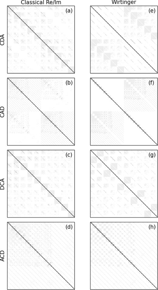
$A graphical representation of ${\bf J}$H${\bf J}$ for a case of 40 antennas and five directions. Each pixel represents the amplitude of a single matrix element. The left-hand column (a)–(d) shows conventional real-only Jacobians constructed by taking the partial derivatives with respect to the real and imaginary parts of the gains. The ordering of the parameters is (a) real/imaginary major, direction, antenna minor (i.e. antenna changes fastest); (b) real/imaginary, antenna, direction; (c) direction, real/imaginary, antenna; (d) antenna, real/imaginary, direction. The right-hand column (e)–(h) shows full complex Jacobians with similar parameter ordering (direct/conjugate instead of real/imaginary). Note that panel (f) can also be taken to represent the DI case, if we imagine each 5 × 5 block as 1 pixel.$

Figure 1.

A graphical representation of |${\bf J}$|^H|${\bf J}$| for a case of 40 antennas and five directions. Each pixel represents the amplitude of a single matrix element. The left-hand column (a)–(d) shows conventional real-only Jacobians constructed by taking the partial derivatives with respect to the real and imaginary parts of the gains. The ordering of the parameters is (a) real/imaginary major, direction, antenna minor (i.e. antenna changes fastest); (b) real/imaginary, antenna, direction; (c) direction, real/imaginary, antenna; (d) antenna, real/imaginary, direction. The right-hand column (e)–(h) shows full complex Jacobians with similar parameter ordering (direct/conjugate instead of real/imaginary). Note that panel (f) can also be taken to represent the DI case, if we imagine each 5 × 5 block as 1 pixel.

Open in new tab Download slide

In Section 4, we show that different algorithms may be derived by combining different sparse approximations to |${\bf J}$|^H|${\bf J}$| with conventional GN and LM methods. In particular, we show that StefCal, a fast DI calibration algorithm recently proposed by Salvini & Wijnholds (2014a), can be straightforwardly derived from a diagonal approximation to a complex |${\bf J}$|^H|${\bf J}$|⁠. We show that the complex Jacobian approach naturally extends to the DD case, and that other sparse approximations yield a whole family of DD calibration algorithms with different scaling properties. One such algorithm, CohJones (Tasse 2014b), has been implemented and successfully applied to simulated Low Frequency Array (LOFAR) data: this is discussed in Section 7.

In Section 5, we extend this approach to the fully polarized case, by developing a Wirtinger-like operator calculus in which the polarization problem can be formulated succinctly. This naturally yields fully polarized counterparts to the calibration algorithms defined previously. In Section 6, we discuss other algorithmic variations, and make connections to older DD calibration techniques such as peeling (Noordam 2004).

While the scope of this work is restricted to LS solutions to the DI and DD gain calibration problem, the potential applicability of complex optimization to radio interferometry is perhaps broader. We will return to this in the conclusions.

2 WIRTINGER CALCULUS AND COMPLEX LEAST SQUARES

The traditional approach to optimizing a function of n complex variables |$f(\boldsymbol {z}),$||$\boldsymbol {z}\in \mathbb {C}^n$| is to treat the real and imaginary parts |$\boldsymbol {z}=\boldsymbol {x}+{\rm i}\boldsymbol {y}$| independently, turning f into a function of 2n real variables |$f(\boldsymbol {x},\boldsymbol {y})$|⁠, and the problem into an optimization over |$\mathbb {R}^{2n}$|⁠.

Kreutz-Delgado (2009) and Laurent et al. (2012) propose an alternative approach to the problem based on Wirtinger (1927) calculus. The central idea of Wirtinger calculus is to treat |$\boldsymbol {z}$| and |$\bar{\boldsymbol {z}}$| as independent variables, and optimize |$f(\boldsymbol {z},\bar{\boldsymbol {z}})$| using the Wirtinger derivatives

\begin{equation} \frac{\mathrm{\partial} }{\mathrm{\partial} z} = \frac{1}{2}\left(\frac{\mathrm{\partial} }{\mathrm{\partial} x} - {\rm i}\frac{\mathrm{\partial} }{\mathrm{\partial} y} \right),\ \quad \frac{\mathrm{\partial} }{\mathrm{\partial} \bar{z}} = \frac{1}{2}\left(\frac{\mathrm{\partial} }{\mathrm{\partial} x} + {\rm i}\frac{\mathrm{\partial} }{\mathrm{\partial} y} \right), \end{equation}

(2.1)

where z = x + iy. It is easy to see that

\begin{equation} \frac{\mathrm{\partial} \bar{z}}{\mathrm{\partial} z} = \frac{\mathrm{\partial} z}{\mathrm{\partial} \bar{z}} = 0, \end{equation}

(2.2)

i.e. that |$\bar{z}$| (z) is treated as constant when taking the derivative with respect to z (⁠|$\bar{z}$|⁠). From this it is straightforward to define the complex gradient operator

\begin{equation} \frac{\mathrm{\partial} }{\mathrm{\partial} ^C \boldsymbol {z}} = \left[ \frac{\mathrm{\partial} }{\mathrm{\partial} \boldsymbol {z}}, \frac{\mathrm{\partial} }{\mathrm{\partial} \bar{\boldsymbol {z}}} \right] = \left[ \frac{\mathrm{\partial} }{\mathrm{\partial} z_1}, \dots , \frac{\mathrm{\partial} }{\mathrm{\partial} z_n}, \frac{\mathrm{\partial} }{\mathrm{\partial} \bar{z}_1}, \dots , \frac{\mathrm{\partial} }{\mathrm{\partial} \bar{z}_n} \right], \end{equation}

(2.3)

from which definitions of the complex Jacobian and complex Hessians naturally follow. The authors then show that various optimization techniques developed for real functions can be reformulated using complex Jacobians and Hessians, and applied to the complex optimization problem. In particular, they generalize the GN and LM methods for solving the NLLS problem:¹

\begin{equation} \min _{\boldsymbol {z}} \Vert \boldsymbol {r}(\boldsymbol {z},\boldsymbol {\bar{z}})\Vert _{\rm F},\ \ \ \mathrm{or}\ \min _{\boldsymbol {z}} \Vert \boldsymbol {d}-\boldsymbol {v}(\boldsymbol {z},\boldsymbol {\bar{z}})\Vert _{\rm F}, \end{equation}

(2.4)

where |$\boldsymbol {r},\ \boldsymbol {d},\ \boldsymbol {v}$| have values in |$\mathbb {C}^m$|⁠, and || · ||_F is the Frobenius norm. The latter form refers to LS fitting of the parametrized model |$\boldsymbol {v}$| to observed data |$\boldsymbol {d}$|⁠, and is the preferred formulation in the context of radio interferometry.

Complex NLLS is implemented as follows. Let us formally treat |$\boldsymbol {z}$| and |$\boldsymbol {\bar{z}}$| as independent variables, define an augmented parameter vector containing both,

\begin{equation} \boldsymbol {\breve{z}}= \left[\begin{array}{@{}c@{}}\boldsymbol {z}\\ \boldsymbol {\bar{z}}\end{array} \right] \end{equation}

(2.5)

and designate its value at step k by |$\boldsymbol {\breve{z}}_k$|⁠. Then, define

\begin{equation} {{\bf J}}_k=\frac{\mathrm{\partial} \boldsymbol {v}}{\mathrm{\partial} \boldsymbol {z}} (\boldsymbol {\breve{z}}_k), \quad {{\bf J}}_{k^*}=\frac{\mathrm{\partial} \boldsymbol {v}}{\mathrm{\partial} \bar{\boldsymbol {z}}}(\boldsymbol {\breve{z}}_k),\quad \boldsymbol {\breve{r}}_k=\left[\begin{array}{@{}c@{}}\boldsymbol {r}(\boldsymbol {\breve{z}}_k)\\ \bar{\boldsymbol {r}}(\boldsymbol {\breve{z}}_k)\end{array} \right]. \end{equation}

(2.6)

We will call the m × n matrices |${\bf J}$|_k and |${{\bf J}}_{k^*}$| the partial and partial conjugate Jacobian,² respectively, and the 2m-vector |$\boldsymbol {\breve{r}}_k$| the augmented residual vector. The complex Jacobian of the model |$\boldsymbol {v}$| can then be written (in block matrix form) as

\begin{equation} {{\bf J}}= \left[\begin{array}{@{}cc@{}}{{\bf J}}_k &\quad {{\bf J}}_{k^*} \\ \bar{{{\bf J}}}_{k^*} &\quad \bar{{{\bf J}}}_{k} \end{array} \right], \end{equation}

(2.7)

with the bottom two blocks being element-by-element conjugated versions of the top two. Note the use of |$\bar{{{\bf J}}}$| to indicate element-by-element conjugation – not to be confused with the Hermitian conjugate which we will invoke later. |${\bf J}$| is a 2m × 2n matrix. The GN update step is defined as

\begin{equation} \delta \boldsymbol {\breve{z}}= \left[\begin{array}{@{}c@{}}\delta \boldsymbol {z}\\ \delta \bar{\boldsymbol {z}}\end{array} \right] = ({{\bf J}}^{\rm H} {{\bf J}})^{-1}{{\bf J}}^{\rm H} \boldsymbol {\breve{r}}_k. \end{equation}

(2.8)

The LM approach is similar, but introduces a damping parameter λ:

\begin{equation} \delta \boldsymbol {\breve{z}}= \left[\begin{array}{@{}c@{}}\delta \boldsymbol {z}\\ \delta \bar{\boldsymbol {z}}\end{array} \right] = ({{\bf J}}^{\rm H} {{\bf J}}+ \lambda {{\bf D}})^{-1}{{\bf J}}^{\rm H} \boldsymbol {\breve{r}}_k, \end{equation}

(2.9)

where |${\bf D}$| is the diagonalized version of |${\bf J}$|^H|${\bf J}$|⁠. With λ = 0 this becomes equivalent to GN, with λ → ∞ this corresponds to steepest descent (SD) with ever smaller steps.

Note that while |$\delta \boldsymbol {z}$| and |$\delta \bar{\boldsymbol {z}}$| are formally computed independently, the structure of the equations is symmetric (since the function being minimized – the Frobenius norm – is real and symmetric with respect to |$\boldsymbol {z}$| and |$\bar{\boldsymbol {z}}$|⁠), which ensures that |$\overline{\delta \boldsymbol {z}} = \delta \bar{\boldsymbol {z}}$|⁠. In practice this redundancy usually means that only half the calculations need to be performed.

Laurent et al. (2012) show that equations (2.8) and (2.9) yield exactly the same system of LS equations as would have been produced had we treated |$\boldsymbol {r}(\boldsymbol {z})$| as a function of real and imaginary parts |$\boldsymbol {r}(\boldsymbol {x},\boldsymbol {y})$|⁠, and taken ordinary derivatives in |$\mathbb {R}^{2n}$|⁠. However, the complex Jacobian may be easier and more elegant to derive analytically, as we will see below in the case of radio interferometric calibration.

3 SCALAR (UNPOLARIZED) CALIBRATION

In this section we will apply the formalism above to the scalar case, i.e. that of unpolarized calibration. This will then be extended to the fully polarized case in Section 5.

3.1 Direction-independent calibration

Let us first explore the simplest case of DI calibration. Consider an interferometer array of N_ant antennas measuring N_bl = N_ant(N_ant − 1)/2 pairwise visibilities. Each antenna pair pq (1 ≤ p < q ≤ N_ant) measures the visibility:³

\begin{equation} g_p m_{pq} \bar{g}_q + n_{pq}, \end{equation}

(3.1)

where m_pq is the (assumed known) sky coherency, g_p is the (unknown) complex gain parameter associated with antenna p, and n_pq is a complex noise term that is Gaussian with a mean of 0 in the real and imaginary parts. The calibration problem then consists of estimating the complex antenna gains |$\boldsymbol {g}$| by minimizing residuals in the LS sense:

\begin{equation} \min _{\boldsymbol {g}}\sum _{pq}|r_{pq}|^2,\ \quad \ r_{pq}=d_{pq}-g_p m_{pq} \bar{g}_q, \end{equation}

(3.2)

where d_pq are the observed visibilities. Treating this as a complex optimization problem as per the above, let us write out the complex Jacobian. With a vector of N_ant complex parameters |$\boldsymbol {g}$| and N_bl measurements d_pq, we will have a full complex Jacobian of shape 2N_bl × 2N_ant. It is conventional to think of visibilities laid out in a visibility matrix; the normal approach at this stage is to vectorize d_pq by fixing a numbering convention so as to enumerate all the possible antenna pairs pq (p < q) using numbers from 1 to N_bl. Instead, let us keep using pq as a single ‘compound index’, with the implicit understanding that pq in subscript corresponds to a single index from 1 to N_bl using some fixed enumeration convention. Where necessary, we will write pq in square brackets (e.g. a_{[pq], i}) to emphasize this.

Now consider the corresponding partial Jacobian |${\bf J}$|_k matrix (equation 2.6). This is of shape N_bl × N_ant. Using the Wirtinger derivative, we can write the partial Jacobian in terms of its value at row [pq] and column j as

\begin{equation} [ {{\bf J}}_k ]_{[pq],j} = \left\lbrace \begin{array}{ll}m_{pq}\bar{g}_q,&\quad j=p, \\ 0, &\quad \mathrm{otherwise.} \end{array} \right. \end{equation}

(3.3)

In other words, within each column j, |${\bf J}$|_k is only non-zero at rows corresponding to baselines [jq]. We can express this more compactly using the Kronecker δ:

\begin{equation} J_k = \overbrace{ \left[\begin{array}{@{}c@{}}m_{pq}\bar{g}_q\delta ^{j}_p \end{array} \right] } ^{j=1\dots N_\mathrm{ant}} \boldsymbol { \rbrace } {\scriptstyle [pq]=1\dots N_\mathrm{bl}\ (p<q)}. \end{equation}

(3.4)

Likewise, the conjugate partial Jacobian |$J_{k^*}$| may be written as

\begin{equation} J_{k^*} = \overbrace{ \left[\begin{array}{@{}c@{}}g_p m_{pq} \delta ^{j}_q \end{array} \right] } ^{j=1\dots N_\mathrm{ant}} \boldsymbol { \rbrace } {\scriptstyle [pq]=1\dots N_\mathrm{bl}\ (p<q)}. \end{equation}

(3.5)

A specific example is provided in Appendix A. The full complex Jacobian (equation 2.7) then becomes, in block matrix notation,

\begin{equation} \begin{array}{r@{\ }cc@{\ }cc}&\overbrace{\ \ \ \ \ \ \ \ }^{j=1\dots N_\mathrm{ant}} &\quad \overbrace{\ \ \ \ \ \ \ \ }^{j=1\dots N_\mathrm{ant}} \\ {{\bf J}}= \bigg [ &\begin{array}{@{}c@{}}m_{pq}\bar{g}_q\delta ^{j}_p \\ \bar{m}_{pq} \bar{g}_p \delta ^{j}_q \end{array} &\quad \begin{array}{@{}c@{}}g_p m_{pq} \delta ^{j}_q \\ g_q \bar{m}_{pq} \delta ^{j}_p \end{array} &\bigg ] &\quad \begin{array}{@{}c@{}}\boldsymbol {\rbrace } {\scriptstyle [pq]=1\dots N_\mathrm{bl}}\ (p<q), \\ \boldsymbol {\rbrace } {\scriptstyle [pq]=1\dots N_\mathrm{bl}}\ (p<q), \end{array} \end{array} \end{equation}

(3.6)

where the [pq] (p < q) and j superscripts within each block span the full range of 1…N_bl and 1…N_ant. Now, since |$d_{pq} = \bar{d}_{qp}$| and |$m_{pq} = \bar{m}_{qp}$|⁠, we may notice that the bottom half of the augmented residuals vector |$\boldsymbol {\breve{r}}$| corresponds to the conjugate baselines qp (q > p):

\begin{equation} \boldsymbol {\breve{r}}= \left[\begin{array}{@{}c@{}}r_{pq} \\ \bar{r}_{pq} \end{array} \right] = \left[\begin{array}{@{}c@{}}d_{pq}-g_p m_{pq}\bar{g}_q\\ \bar{d}_{pq}-\bar{g}_p \bar{m}_{pq}g_q\end{array} \right] = \left[\begin{array}{@{}c@{}}r_{pq} \\ r_{qp} \end{array} \right]\ \ \begin{array}{@{}c@{}}\boldsymbol {\rbrace } \scriptstyle [pq]=1\dots N_\mathrm{bl}\ (p<q), \\ \boldsymbol {\rbrace } \scriptstyle [pq]=1\dots N_\mathrm{bl}\ (p<q), \end{array} \end{equation}

(3.7)

as does the bottom half of |${\bf J}$| in equation (3.6). Note that we are free to reorder the rows of |${\bf J}$| and |$\boldsymbol {\breve{r}}$| and intermix the normal and conjugate baselines, as this will not affect the LS equations derived at equation (2.9). This proves most convenient: instead of splitting |${\bf J}$| and |$\boldsymbol {\breve{r}}$| into two vertical blocks with the compound index [pq] (p < q) running through N_bl rows within each block, we can treat the two blocks as one, with a single compound index [pq] (p ≠ q) running through 2N_bl rows:

\begin{equation} \begin{array}{r@{\ }cc@{\ }cc}& \overbrace{\ \ \ \ \ \ \ \ }^{j=1\dots N_\mathrm{ant}} &\quad \overbrace{\ \ \ \ \ \ \ \ }^{j=1\dots N_\mathrm{ant}} \\ {{\bf J}}= \big [ & m_{pq}\bar{g}_q\delta ^{j}_p &\quad g_p m_{pq} \delta ^{j}_q & \big ],\ \boldsymbol {\breve{r}}= [ r_{pq} ] \ \ {\boldsymbol {\rbrace } \scriptstyle [pq]=1\dots 2N_\mathrm{bl}}, \end{array} \end{equation}

(3.8)

where for q > p, |$r_{pq}=\bar{r}_{qp}$|⁠, and |$m_{pq}=\bar{m}_{qp}$|⁠. For clarity, we may adopt the following order for enumerating the row index [pq]: 12, 13, …, 1n, 21, 22, …, 2n, 31, 32, …, 3n, …, n1, …, n n − 1.

Equation (A2) in Appendix A provides an example of |${\bf J}$| for the three-antenna case. For brevity, let us define the shorthand

\begin{equation} y_{pq} = m_{pq} \bar{g}_q. \end{equation}

(3.9)

We can now write out the structure of |${\bf J}$|^H|${\bf J}$|⁠. This is Hermitian, consisting of four N_ant × N_ant blocks:

\begin{equation} {{\bf J}}^{\rm H}{{\bf J}}= \left[\begin{array}{@{}cc@{}}{{\bf A}}&\quad{{\bf B}}\\ {{\bf C}}&\quad{{\bf D}}\end{array} \right] = \left[\begin{array}{@{}cc@{}}{{\bf A}}&\quad{{\bf B}}\\ {{\bf B}}^{\rm H}&\quad{{\bf A}}\end{array} \right], \end{equation}

(3.10)

since the value at row i, column j of each block is

\begin{eqnarray} A_{ij} = \sum _{pq} \bar{y}_{pq} y_{pq} \delta ^{i}_p \delta ^{j}_p &=& \left\lbrace \begin{array}{cc}\sum \limits _{q\ne i} |y_{iq}^2|, &\quad \scriptstyle i=j, \\ \!\!\!\!\!\!\!\!\!0, &\quad \scriptstyle i\ne j, \end{array} \right.\nonumber \\ B_{ij} = \sum _{pq} \bar{y}_{pq} \bar{y}_{qp} \delta ^{i}_p \delta ^{j}_q &=& \left\lbrace \begin{array}{cc}\bar{y}_{ij} \bar{y}_{ji}, &\quad \scriptstyle i\ne j,\\ \!\!\!\!\!\!0, &\quad \scriptstyle i=j, \end{array} \right.\nonumber \\ C_{ij} = \sum _{pq} y_{qp} y_{pq} \delta ^{i}_q \delta ^{j}_p &=& \bar{B}_{ij}, \nonumber \\ D_{ij} = \sum _{pq} y_{pq} \bar{y}_{pq} \delta ^{i}_q \delta ^{j}_q &=& A_{ij}. \end{eqnarray}

(3.11)

We then write |${\bf J}$|^H|${\bf J}$| in terms of the four N_ant × N_ant blocks as

\begin{equation} {{\bf J}}^{\rm H} {{\bf J}}= \left[\begin{array}{@{}c@{\quad }|@{\quad }c@{}} \mathrm{diag} \sum \limits _{q\ne i} |y_{iq}^2| & \left\lbrace \begin{array}{@{}c@{\quad}c@{}} \bar{y}_{ij} \bar{y}_{ji}, & {\scriptstyle i\ne j} \\ 0, & {\scriptstyle i=j} \end{array} \right. \\ {\cdots\cdots\cdots\cdots\cdots\cdots\cdots\cdots\cdots} \\ \left\lbrace \begin{array}{@{}c@{\quad}c@{}} y_{ij}y_{ji},& {\scriptstyle i\ne j} \\ 0, & {\scriptstyle i=j} \end{array} \right. & \mathrm{diag} \sum \limits _{q\ne i} |y^2_{iq}| \end{array} \right] . \end{equation}

(3.12)

Equation (A3) in Appendix A provides an example of |${\bf J}$|^H|${\bf J}$| for the three-antenna case.

The other component of the LM/GN equations (equation 2.9) is the |${{\bf J}}^{\rm H}\boldsymbol {\breve{r}}$| term. This will be a column vector of length 2N_ant. We can write this as a stack of two N_ant vectors:

\begin{equation} {{\bf J}}^{\rm H}\boldsymbol {\breve{r}}= \left[\begin{array}{@{}c@{}}\sum \limits _{pq} \bar{y}_{pq} r_{pq} \delta ^{i}_p \\ \sum \limits _{pq} y_{qp} r_{pq} \delta ^{i}_q \end{array} \right] = \left[\begin{array}{@{}c@{}}\sum \limits _{q\ne i} \bar{y}_{iq} r_{iq} \\ \sum \limits _{q\ne i} y_{iq} \bar{r}_{iq} \end{array} \right] \begin{array}{@{}c@{}}\boldsymbol {\big \rbrace } \scriptstyle i=1\dots N_\mathrm{ant}, \\ \boldsymbol {\big \rbrace } \scriptstyle i=1\dots N_\mathrm{ant}, \end{array} \end{equation}

(3.13)

with the second equality established by swapping p and q in the bottom sum, and making use of |$r_{pq}=\bar{r}_{qp}$|⁠. Clearly, the bottom half of the vector is the conjugate of the top:

\begin{equation} {{\bf J}}^{\rm H}\boldsymbol {\breve{r}}= \left[\begin{array}{@{}c@{}} \boldsymbol {c}\\ \bar{\boldsymbol {c}}\end{array} \right],\ \quad c_i = \sum \limits _{q\ne i} \bar{y}_{iq} r_{iq}. \end{equation}

(3.14)

3.2 Computing the parameter update

Because of the structure of the RIME, we have a particularly elegant way of computing the GN update step. By analogy with the augmented residuals vector |$\boldsymbol {\breve{r}}$|⁠, we can express the data and model visibilities as 2N_bl vectors, using the compound index [pq] (p ≠ q):

\begin{equation} \boldsymbol {\breve{d}}= [ d_{pq} ],\ \quad \boldsymbol {\breve{v}}= [ g_p m_{pq} \bar{g}_q ],\ \quad \boldsymbol {\breve{r}}=\boldsymbol {\breve{d}}-\boldsymbol {\breve{v}}. \end{equation}

(3.15)

As noted by Tasse (2014b), we have the wonderful property that

\begin{equation} \boldsymbol {\breve{v}}= {{\bf J}}_\mathrm{L}\boldsymbol {g} = \frac{1}{2}{{\bf J}}\boldsymbol {\breve{g}},\ \ \ \mathrm{where}\ \boldsymbol {\breve{g}}= \left[\begin{array}{@{}c@{}} \boldsymbol {g} \\ \boldsymbol {\bar{g}}\end{array} \right] \end{equation}

(3.16)

(where |$\boldsymbol {X}_\mathrm{L}$| designates the left half of matrix |$\boldsymbol {X}$| – see Table 1 for a summary of notation), which basically comes about due to the RIME being bilinear with respect to |$\boldsymbol {g}$| and |$\boldsymbol {\bar{g}}$|⁠. Substituting this into the GN update step, and noting that |$\boldsymbol {X}(\boldsymbol {Y}_\mathrm{L}) = (\boldsymbol {XY})_\mathrm{L}$|⁠, we have

\begin{equation} \left[\begin{array}{@{}c@{}} \delta \boldsymbol {g}\\ \delta \boldsymbol {\bar{g}}\end{array} \right] = ({{\bf J}}^{\rm H}{{\bf J}})^{-1} {{\bf J}}^{\rm H} (\boldsymbol {\breve{d}}- {{\bf J}}_\mathrm{L}\boldsymbol {g}) = ({{\bf J}}^{\rm H}{{\bf J}})^{-1} {{\bf J}}^{\rm H} \boldsymbol {\breve{d}}- \boldsymbol {g}. \end{equation}

(3.17)

Consequently, the updated gain values at each iteration can be derived directly from the data, thus obviating the need for computing residuals. Additionally, since the bottom half of the equations is simply the conjugate of the top, we only need to evaluate the top half:

\begin{equation} \boldsymbol {g}_{k+1} = \boldsymbol {g}_k + \delta \boldsymbol {g}= ({{\bf J}}^{\rm H}{{\bf J}})^{-1}_{\ \ \ \mathrm{U}} {{\bf J}}^{\rm H} \boldsymbol {\breve{d}}, \end{equation}

(3.18)

where |$\boldsymbol {X}_\mathrm{U}$| designates the upper half of matrix |$\boldsymbol {X}$|⁠.

The derivation above assumes an exact inversion of |${\bf H}$| = |${\bf J}$|^H|${\bf J}$|⁠. In practice, this large matrix can be costly to invert, so the algorithms below will substitute it with some cheaper-to-invert approximation |$\tilde{{{\bf H}}}$|⁠. Using the approximate matrix in the GN update equation, we find instead that

\begin{equation} \boldsymbol {g}_{k+1} = \tilde{{{\bf H}}}^{-1}_{\ \ \ \mathrm{U}} {{\bf J}}^{\rm H} \boldsymbol {\breve{d}}+ (\mathbb {I}- \tilde{{{\bf H}}}^{-1}_{\ \ \ \mathrm{U}} {{\bf H}}_\mathrm{L})\boldsymbol {g}_k, \end{equation}

(3.19)

which means that when an approximate |${\bf J}$|^H|${\bf J}$| is in use, the shortcut of equation (3.18) only applies when

\begin{equation} \tilde{{{\bf H}}}^{-1}_{\ \ \ \mathrm{U}} {{\bf H}}_\mathrm{L}=\mathbb {I}. \end{equation}

(3.20)

We will see examples of both conditions below, so it is worth stressing the difference: equation (3.18) allows us to compute updated solutions directly from the data vector, bypassing the residuals. This is a substantial computational shortcut, however, when an approximate inverse for |${\bf H}$| is in use, it does not necessarily apply (or at least is not exact). Under the condition of equation (3.20), however, such a shortcut is exact.

3.3 Time/frequency solution intervals

A common use case [especially in low signal-to-noise ratio (SNR) scenarios] is to employ larger solution intervals. That is, we measure multiple visibilities per each baseline pq, across an interval of time slots and frequency channels, then obtain complex gain solutions that are constant across each interval. The minimization problem of equation (3.1) can then be rewritten as

\begin{equation} \min _{\boldsymbol {g}}\sum _{pqs}|r_{pqs}|^2, \ \ \ r_{pqs} = d_{pqs}-g_p m_{pqs} \bar{g}_q, \end{equation}

(3.21)

where s = 1, …, N_s is a sample index enumerating all the samples within the time/frequency solution interval. We can repeat the derivations above using [pqs] as a single compound index. Instead of having shape 2N_bl × 2N_ant, the Jacobian will have a shape of 2N_blN_s × 2N_ant, and the residual vector will have a length of 2N_blN_s. In deriving the |${\bf J}$|^H|${\bf J}$| term, the sums in equation (3.10) must be taken over all pqs rather than just pq. Defining the usual shorthand of |$y_{pqs}=m_{pqs}\bar{g}_q$|⁠, we then have

\begin{equation} {{\bf J}}^{\rm H} {{\bf J}}= \left[\begin{array}{c@{\quad }|@{\quad }c} \mathrm{diag} \sum \limits _{q\ne i,s} |y^2_{iqs}| & \nearrow ^{\rm H}\;\;\\ {\cdots\cdots\cdots\cdots\cdots\cdots\cdots\cdots\cdots} \\ \left\lbrace \begin{array}{ccc} \sum \limits _{s} y_{ijs}y_{jis},&\quad{\scriptstyle i\ne j} \\ 0, &\quad{\scriptstyle i=j} \end{array} \right. & \searrow \end{array} \right] , \end{equation}

(3.22)

where the symbols ↘ and ↗^H represent a copy and a copy-transpose of the appropriate matrix block (as per the structure of equation 3.10). Likewise, the |${{\bf J}}^{\rm H}\boldsymbol {\breve{r}}$| term can be written as

\begin{equation} {{\bf J}}^{\rm H}\boldsymbol {\breve{r}}= \left[\begin{array}{@{}c@{}} \sum \limits _{q\ne i,s} \bar{y}_{iqs} r_{iqs} \\ \cdots\cdots\cdots\cdots\cdots\\ \downarrow ^{\rm H} \end{array} \right]. \end{equation}

(3.23)

3.4 Weighting

Although Laurent et al. (2012) do not mention this explicitly, it is straightforward to incorporate weights into the complex LS problem. Equation (2.4) is reformulated as

\begin{equation} \min _{\boldsymbol {z}} \Vert {{\bf W}} \boldsymbol {\breve{r}}(\boldsymbol {z},\boldsymbol {\bar{z}})\Vert _{\rm F}, \end{equation}

(3.24)

where |${\bf W}$| is an M × M weights matrix (usually, the inverse of the data covariance matrix |${\bf C}$|⁠). This then propagates into the LM equations as

\begin{equation} \delta \boldsymbol {\breve{z}}= ({{\bf J}}^{\rm H} {{\bf W}} {{\bf J}}+ \lambda \mathbb {I})^{-1}{{\bf J}}^{\rm H} {{\bf W}} \boldsymbol {\breve{r}}_k. \end{equation}

(3.25)

Adding weights to equations (3.22) and (3.23), we arrive at the following:

\begin{equation} {{\bf J}}^{\rm H}{{\bf W}}{{\bf J}}= \left[\begin{array}{c@{\quad }|@{\quad }c} \mathrm{diag} \sum \limits _{q\ne i,s} w_{iqs} |y^2_{iqs}| & \nearrow ^{\rm H} \\ {\cdots\cdots\cdots\cdots\cdots\cdots\cdots\cdots} \\ \left\lbrace \begin{array}{@{}c@{,\ }c@{}} \sum \limits _{s} w_{ijs} y_{ijs}y_{jis}&{\scriptstyle i\ne j} \\ 0 &{\scriptstyle i=j} \end{array} \right. & \searrow \ \ \end{array} \right] , \end{equation}

(3.26)

\begin{equation} {{\bf J}}^{\rm H}{{\bf W}}\boldsymbol {\breve{r}}= \left[\begin{array}{@{}c@{}}\sum \limits _{q\ne i,s} w_{iqs} \bar{y}_{iqs} r_{iqs} \\ \cdots\cdots\cdots\cdots\cdots\cdots \\ \downarrow ^{\rm H} \end{array} \right]. \end{equation}

(3.27)

3.5 Direction-dependent calibration

Let us apply the same formalism to the DD calibration problem. We reformulate the sky model as a sum of N_dir sky components, each with its own DD gain. It has been common practice to do DD gain solutions on larger time/frequency intervals than DI solutions, both for SNR reasons, and because short intervals lead to underconstrained solutions and suppression of unmodelled sources. We therefore incorporate solution intervals into the equations from the beginning. The minimization problem becomes

\begin{equation} \min _{\boldsymbol {g}}\sum _{pqs}|r_{pqs}|^2, \ \ \ r_{pqs} = d_{pqs} - \sum _{d=1}^{N_\mathrm{dir}} g^{(d)}_p m^{(d)}_{pqs} \bar{g}^{(d)}_q. \end{equation}

(3.28)

It is obvious that the Jacobian corresponding to this problem is very similar to the one in equation (3.8), but instead of having shape 2N_bl × 2N_ant, this will have a shape of 2N_blN_s × 2N_antN_dir. We now treat [pqs] and [jd] as compound indices:

\begin{equation} \begin{array}{r@{\ }cc@{\ }cc}& \overbrace{\ \ \ \ \ \ \ \ \ \ \ \ }^{\begin{array}{@{}c@{}}\scriptstyle j=1\dots N_\mathrm{ant}\\ \scriptstyle d=1\dots N_\mathrm{dir}\end{array}} & \overbrace{\ \ \ \ \ \ \ \ \ \ \ \ }^{\begin{array}{@{}c@{}}\scriptstyle j=1\dots N_\mathrm{ant}\\ \scriptstyle d=1\dots N_\mathrm{dir}\end{array}} \\ {{\bf J}}= \bigg [ & m^{(d)}_{pqs}\bar{g}^{(d)}_q \delta ^j_p &\quad g^{(d)}_p m^{(d)}_{pqs} \delta ^j_q \bigg ] & \boldsymbol {\bigg \rbrace } \begin{array}{l}\scriptstyle [pq]=1\dots 2N_\mathrm{bl}\ (p\ne q),\\ \scriptstyle s=1\dots N_s. \end{array} \end{array} \end{equation}

(3.29)

Every antenna j and direction d will correspond to a column in |${\bf J}$|⁠, but the specific order of the columns (corresponding to the order in which we place the |$g^{(d)}_p$| elements in the augmented parameter vector |$\boldsymbol {\breve{g}}$|⁠) is completely up to us.

Consider now the |${\bf J}$|^H|${\bf J}$| product. This will consist of 2 × 2 blocks, each of shape [N_antN_dir]². Let us use i, c to designate the rows within each block, j, d to designate the columns, and define |$y^{(d)}_{pqs}=m^{(d)}_{pqs}\bar{g}^{(d)}_q$|⁠. The |${\bf J}$|^H|${\bf J}$| matrix will then have the following block structure:

\begin{eqnarray} {{\bf J}}^{\rm H}{{\bf J}}= \left[\begin{array}{cc} {\bf A} & {\bf B}^{\rm H}\\ {\bf B} & {\bf A} \end{array} \right] = \left[\begin{array}{c@{\quad }|@{\quad }c} \delta ^i_j \sum \limits _{q\ne i,s} \bar{y}^{(c)}_{iqs} y^{(d)}_{iqs} & \nearrow ^{\rm H}\nonumber\\ {\cdots\cdots\cdots\cdots\cdots\cdots\cdots\cdots\cdots} \nonumber\\ \left\lbrace \begin{array}{@{}c@{}c@{}c@{}}\sum \limits _{s} y^{(c)}_{jis} y^{(d)}_{ijs},\quad{\scriptstyle i\ne j} \nonumber\\ 0, &\quad{\scriptstyle i=j} \end{array} \right. & \searrow \ \ \end{array}\right] , \nonumber\\ \end{eqnarray}

(3.30)

while the |${{\bf J}}^{\rm H}\boldsymbol {\breve{r}}$| term will be a vector of length 2N_antN_dir, with the bottom half again being a conjugate of the top half. Within each half, we can write out the element corresponding to antenna j, direction d:

\begin{equation} {{\bf J}}^{\rm H}\boldsymbol {\breve{r}}= \left[\begin{array}{@{}c@{}}\boldsymbol {c}\\ \bar{\boldsymbol {c}}\end{array} \right],\ \quad c_{jd} = \sum \limits _{q\ne j,s} \bar{y}^{(d)}_{jqs} r_{jqs}. \end{equation}

(3.31)

Finally, let us note that the property of equation (3.16) also holds for the DD case. It is easy to see that

\begin{equation} \boldsymbol {\breve{v}}= \bigg [ \sum _{d=1}^{N_\mathrm{dir}} g^{(d)}_p m^{(d)}_{pqs} \bar{g}^{(d)}_q \bigg ] = {{\bf J}}_\mathrm{L}\boldsymbol {\breve{g}}. \end{equation}

(3.32)

Consequently, the shortcut of equation (3.18) also applies.

4 INVERTING |$\boldsymbol {{{\bf J}}^{\rm H}{{\bf J}}}$| AND SEPARABILITY

In principle, implementing one of the flavours of calibration above is ‘just’ a matter of plugging equations (3.12)+(3.14), (3.22)+(3.23), (3.26)+(3.27), or (3.30)+3.31 into one the algorithms defined in Appendix C. Note, however, that both the GN and LM algorithms hinge around inverting a large matrix. This will have a size of 2N_ant or 2N_antN_dir squared for the DI or DD case, respectively. With a naive implementation of matrix inversion, which scales cubically, algorithmic costs become dominated by the |$O(N_\mathrm{ant}^3)$| or |$O(N_\mathrm{ant}^3N_\mathrm{dir}^3)$| cost of inversion.

In this section we investigate approaches to simplifying the inversion problem by approximating |${\bf H}$| = |${\bf J}$|^H|${\bf J}$| by some form of (block-) diagonal matrix |$\tilde{{{\bf H}}}$|⁠. Such approximation is equivalent to separating the optimization problem into subsets of parameters that are treated as independent. We will show that some of these approximations are similar to or even fully equivalent to previously proposed algorithms, while others produce new algorithmic variations.

4.1 Diagonal approximation and StefCal

Let us first consider the DI case. The structure of |${\bf J}$|^H|${\bf J}$| in equation (3.12) suggests that it is diagonally dominant (especially for larger N_ant), as each diagonal element is a coherent sum of N_ant amplitude-squared y-terms, while the off-diagonal elements are either zero or a product of two y terms. This is graphically illustrated in Fig. 1(f). It is therefore not unreasonable to approximate |${\bf J}$|^H|${\bf J}$| with a diagonal matrix for purposes of inversion (or equivalently, making the assumption that the problem is separable per antenna):

\begin{equation} \tilde{{{\bf H}}}= \left[\begin{array}{@{}cc@{}} {\bf A} &\quad {0}\\ {0} &\quad {\bf A}\end{array} \right]. \end{equation}

(4.1)

This makes the costs of matrix inversion negligible – O(N_ant) operations, as compared to the |$O(N_\mathrm{ant}^2)$| cost of computing the diagonal elements of the Jacobian in the first place. The price of using an approximate inverse for |${\bf J}$|^H|${\bf J}$| is a less accurate update step, so we can expect to require more iterations before convergence is reached.

Combining this approximation with GN optimization and using equation (3.19), we find the following expression for the GN update step:

\begin{equation} \boldsymbol {g}_{k+1} = \tilde{{{\bf H}}}^{-1}_{\mathrm{UL}} {{\bf J}}_\mathrm{L}^{\, \rm H} \boldsymbol {\breve{d}}, \end{equation}

(4.2)

where |$\boldsymbol {X}_\mathrm{UL}$| designates the top left quadrant of matrix |$\boldsymbol {X}$|⁠. Note that the condition of equation (3.20) is met: |$\tilde{{{\bf H}}}^{-1}_{\ \ \ \mathrm{U}} {{\bf H}}_\mathrm{L}={\bf A}^{-1}{\bf A}=\mathbb {I}$|⁠, i.e. the GN update can be written in terms of |$\boldsymbol {\breve{d}}$|⁠. This comes about due to (i) the off-diagonal blocks of |$\tilde{{{\bf H}}}$| being null, which masks out the bottom half of |${\bf H}$|_L, and (ii) the on-diagonal blocks of |$\tilde{{{\bf H}}}$| being an exact inverse. In other algorithms suggested below, the second condition particularly is not the case.

The per-element expression, in the diagonal approximation, is

\begin{equation} g_{p,k+1} = \left( \sum \limits _{q\ne p} \bar{y}_{pq} y_{pq} \right)^{-1} \sum \limits _{q\ne p} \bar{y}_{pq} d_{pq}. \end{equation}

(4.3)

Equation (4.3) is identical to the update step proposed by Hamaker (2000), and later adopted by Mitchell et al. (2008) for Murchison Widefield Array (MWA) calibration, and independently derived by Salvini & Wijnholds (2014a) for the StefCal algorithm. Note that these authors arrive at the result from a different direction, by treating equation (3.2) as a function of |$\boldsymbol {g}$| only, and completely ignoring the conjugate term. The resulting complex Jacobian (equation 3.6) then has null off-diagonal blocks, and |${\bf J}$|^H|${\bf J}$| becomes diagonal.

Interestingly, applying the same idea to LM optimization (equation 2.9), and remembering that |$\tilde{{{\bf H}}}$| is diagonal, we can derive the following update equation instead:

\begin{equation} \boldsymbol {g}_{k+1} = \frac{\lambda }{1+\lambda }\boldsymbol {g}_k + \frac{1}{1+\lambda } \tilde{{{\bf H}}}_{\mathrm{UL}}^{-1} {{\bf J}}_\mathrm{L}^{\, \rm H} \boldsymbol {\breve{d}}, \end{equation}

(4.4)

which for λ = 1 essentially becomes the basic average-update step of StefCal. We should note that Salvini & Wijnholds (2014a) empirically find better convergence when equation (4.2) is employed for odd k, and equation (4.4) for even k. In terms of the framework defined here, the basic StefCal algorithm can be succinctly described as complex optimization with a diagonally approximated|${\bf J}$|^H|${\bf J}$|⁠, using GN for the odd steps, and LM (λ = 1) for the even steps.

Establishing this equivalence is very useful for our purposes, since the convergence properties of StefCal have been thoroughly explored by Salvini & Wijnholds (2014a), and we can therefore hope to apply these lessons here. In particular, these authors have shown that a direct application of GN produces very slow (oscillating) convergence, whereas combining GN and LM leads to faster convergence. They also propose a number of variations of the algorithm, all of which are directly applicable to the above.

Finally, let us note in passing that the update step of equation (4.3) is embarrassingly parallel, in the sense that the update for each antenna is computed entirely independently.

4.2 Separability of the direction-dependent case

Now consider the problem of inverting |${\bf J}$|^H|${\bf J}$| in the DD case. This is a massive matrix, and a brute force approach would scale as |$O(N_\mathrm{dir}^3N_\mathrm{ant}^3)$|⁠. We can, however, adopt a few approximations. Note again that we are free to reorder our augmented parameter vector (which contains both |$\boldsymbol {g}$| and |$\boldsymbol {\bar{g}}$|⁠), as long as we reorder the rows and columns of |${\bf J}$|^H|${\bf J}$| accordingly.

Let us consider a number of orderings for |$\boldsymbol {\breve{g}}$|⁠:

conjugate major, direction, antenna minor (CDA):
\begin{eqnarray} \left[g^{(1)}_1 \dots g^{(1)}_{N_\mathrm{ant}}, g^{(2)}_1 \dots g^{(2)}_{N_\mathrm{ant}}, g^{(3)}_1 \dots g^{(N_\mathrm{dir})}_{N_\mathrm{ant}}, \bar{g}^{(1)}_1 \dots \bar{g}^{(1)}_{N_\mathrm{ant}} \dots \right]^{\rm T}; \end{eqnarray}
(4.5)
conjugate, antenna, direction (CAD):
\begin{equation} \left[g^{(1)}_1 \dots g^{(N_\mathrm{dir})}_1, g^{(1)}_2 \dots g^{(N_\mathrm{dir})}_2, g^{(1)}_3 \dots g^{(N_\mathrm{dir})}_{N_\mathrm{ant}}, \bar{g}^{(1)}_1 \dots \right]^{\rm T}; \end{equation}
(4.6)
direction, conjugate, antenna (DCA):
\begin{equation} \left[g^{(1)}_1 \dots g^{(1)}_{N_\mathrm{ant}},\bar{g}^{(1)}_1 \dots \bar{g}^{(1)}_{N_\mathrm{ant}}, g^{(2)}_1 \dots g^{(2)}_{N_\mathrm{ant}}, \bar{g}^{(2)}_1 \dots \right]^{\rm T}; \end{equation}
(4.7)
antenna, conjugate, direction (ACD):
\begin{equation} \left[g^{(1)}_1 \dots g^{(N_\mathrm{dir})}_1,\bar{g}^{(1)}_1 \dots \bar{g}^{(N_\mathrm{dir})}_1, g^{(1)}_2 \dots g^{(N_\mathrm{dir})}_2, \bar{g}^{(1)}_2 \dots \right]^{\rm T}. \end{equation}
(4.8)

Figs 1(e)–(h) graphically illustrates the structure of the Jacobian under these orderings.

At this point we may derive a whole family of DD calibration algorithms – there are many ways to skin a cat. Each algorithm is defined by picking an ordering for |$\boldsymbol {\breve{g}}$|⁠, then examining the corresponding |${\bf J}$|^H|${\bf J}$| structure and specifying an approximate matrix inversion mechanism, then applying GN or LM optimization. Let us now work through a couple of examples.

4.2.1 DCA: separating by direction

Let us first consider the DCA ordering (Fig. 1 g). The |${\bf J}$|^H|${\bf J}$| term can be split into N_dir × N_dir blocks:

\begin{equation} {{\bf J}}^{\rm H}{{\bf J}}= \left[\begin{array}{@{}c@{\quad}c@{\quad}c@{}}\mathcal {J}^1_1 & \dots & \mathcal {J}^{N_\mathrm{dir}}_1 \\ \vdots & & \vdots \\ \mathcal {J}_{N_\mathrm{dir}}^1 & \dots & \mathcal {J}_{N_\mathrm{dir}}^{N_\mathrm{dir}} \end{array} \right], \end{equation}

(4.9)

where the structure of each 2N_ant × 2N_ant block at row c, column d, is exactly as given by equation (3.30) (or by Fig. 1f, in miniature).

The on-diagonal (‘same-direction’) blocks |$\mathcal {J}^d_d$| will have the same structure as in the DI case (equation 3.12 or equation A3). Consider now the off-diagonal (‘cross-direction’) blocks |$\mathcal {J}^d_c$|⁠. Their non-zero elements can take one of two forms:

\begin{equation} \sum \limits _{q\ne i,s} \bar{y}^{(c)}_{iqs} y^{(d)}_{iqs} = \sum \limits _{q\ne i} g^{(c)}_q \bar{g}^{(d)}_q \sum _s \bar{m}^{(c)}_{iqs} m^{(d)}_{iqs} \end{equation}

(4.10)

or

\begin{equation} \sum \limits _{s} y^{(c)}_{jis} y^{(d)}_{ijs} = \bar{g}^{(c)}_i \bar{g}^{(d)}_j \sum _s \bar{m}^{(c)}_{ijs} m^{(d)}_{ijs}. \end{equation}

(4.11)

A common element of both is essentially a dot product of sky model components. This is a measure of how ‘non-orthogonal’ the components are:

\begin{equation} X_{pq}^{(cd)} = \left\langle \boldsymbol {m}_{pq}^{(c)},\boldsymbol {m}^{(d)}_{pq} \right\rangle = \sum _s m^{(c)}_{pqs} \bar{m}^{(d)}_{pqs}. \end{equation}

(4.12)

We should now note that each model component will typically correspond to a source of limited extent. This can be expressed as

\begin{equation} m_{pqt\nu }^{(d)} = S^{(d)}_{pqt\nu } k^{(d)}_{pqt\nu }, \end{equation}

(4.13)

where the term S represents the visibility of that sky model component if placed at phase centre (usually only weakly dependent on t, ν – in the case of a point source, for example, S is just a constant flux term), while the term

\begin{equation} k^{(d)}_{pqt\nu } = {\rm e}^{-2\pi {\rm i} (\boldsymbol {u}_{pq}(t)\cdot \boldsymbol {\sigma }_d)\nu /c},\ \ \ \boldsymbol {\sigma }_d = [l_d,m_d,n_d-1]^{\rm T}, \end{equation}

(4.14)

represents the phase rotation to direction |$\boldsymbol {\sigma }_d$| (where lmn are the corresponding direction cosines), given a baseline vector as a function of time |$\boldsymbol {u}_{pq}(t)$|⁠. We can then approximate the sky model dot product above as

\begin{equation} X_{pq}^{(cd)} = S^{(c)}_{pq}S^{(d)}_{pq} \sum _s {\rm e}^{-2\pi {\rm i} [\boldsymbol {u}_{pq}(t)\cdot (\boldsymbol {\sigma }_c-\boldsymbol {\sigma }_d) ]\nu /c}. \end{equation}

(4.15)

The sum over samples s is essentially just an integral over a complex fringe. We may expect this to be small (i.e. the sky model components to be more orthogonal) if the directions are well separated, and also if the sum is taken over longer time and frequency intervals.

If we now assume that the sky model components are orthogonal or near-orthogonal, then we may treat the ‘cross-direction’ blocks of the |${\bf J}$|^H|${\bf J}$| matrix in equation (4.9) as null. The problem is then separable by direction, and |${\bf J}$|^H|${\bf J}$| is approximated by a block-diagonal matrix:

\begin{equation} \tilde{{{\bf H}}}= \left[\begin{array}{@{}c@{\quad}c@{\quad}c@{}}\mathcal {J}^1_1 & & 0 \\ & \ddots & \\ 0 & & \mathcal {J}_{N_\mathrm{dir}}^{N_\mathrm{dir}} \end{array} \right]. \end{equation}

(4.16)

The inversion complexity then reduces to |$O(N_\mathrm{dir}N_\mathrm{ant}^3)$|⁠, which, for large numbers of directions, is a huge improvement on |$O(N_\mathrm{dir}^3N_\mathrm{ant}^3)$|⁠. Either GN or LM optimization may now be applied.

4.2.2 COHJONES: separating by antenna

A complementary approach is to separate the problem by antenna instead. Consider the CAD ordering (Fig. 1f). The top half of |${\bf J}$|^H|${\bf J}$| then has the following block structure (and the bottom half is its symmetric conjugate):

\begin{equation} {{\bf H}}_\mathrm{U}= \left[\begin{array}{@{}c@{\quad}c@{\quad}c@{\quad}c@{\quad}c@{\quad}c@{}} {\bf A}^1_1 & & 0 & {\bf B}^1_1 & \dots & {\bf B}^{N_\mathrm{ant}}_1 \\ & \ddots & & \vdots & & \vdots \\ 0 & & {\bf A}_{N_\mathrm{ant}}^{N_\mathrm{ant}} & {\bf B}_{N_\mathrm{ant}}^1 & \dots & {\bf B}_{N_\mathrm{ant}}^{N_\mathrm{ant}} \end{array} \right], \end{equation}

(4.17)

that is, its left half is block diagonal, consisting of N_dir × N_dir blocks (which follows from equation 3.30), while its right half consists of elements of the form given by equation (4.11).

By analogy with the StefCal approach, we may assume |${\bf B}^i_j \approx 0$|⁠, i.e. treat the problem as separable by antenna. The |$\tilde{{{\bf H}}}$| matrix then becomes block diagonal, and we only need to compute the true matrix inverse of each |${\bf A}^i_i$|⁠. The inversion problem then reduces to |$O(N_\mathrm{dir}^3N_\mathrm{ant})$| in complexity, and either LM or GN optimization may be applied.

For GN, the update step may be computed in direct analogy to equation (4.3) (noting that equation 3.20 holds):

\begin{equation} \boldsymbol {g}_{k+1} = \tilde{{{\bf H}}}_\mathrm{UL}^{-1} {{\bf J}}_\mathrm{L}^{\, \rm H} \boldsymbol {\breve{d}}. \end{equation}

(4.18)

We may note in passing that for LM, the analogy is only approximate:

\begin{equation} \boldsymbol {\breve{g}}_{k+1} \approx \frac{\lambda }{1+\lambda }\boldsymbol {\breve{g}}_k + \frac{1}{1+\lambda } \tilde{{{\bf H}}}_\mathrm{UL}^{-1} {{\bf J}}_\mathrm{L}^{\, \rm H} \boldsymbol {\breve{d}}, \end{equation}

(4.19)

since |$\tilde{{{\bf H}}}$| is only approximately diagonal.

This approach has been implemented as the CohJones (complex half-Jacobian optimization for n-directional estimation) algorithm,⁴ the results of which applied to simulated data are presented below.

4.2.3 ALLJONES: separating all

Perhaps the biggest simplification available is to start with CDA or CAD ordering, and assume a StefCal-style diagonal approximation for the entirety of |${\bf J}$|^H|${\bf J}$|⁠. The matrix then becomes purely diagonal, matrix inversion reduces to O(N_dirN_ant) in complexity, and algorithmic cost becomes dominated by the |$O(N_\mathrm{dir}N_\mathrm{ant}^2)$| process of computing the diagonal elements of |${\bf J}$|^H|${\bf J}$|⁠. Note that equation (3.20) no longer holds, and the GN update step must be computed via the residuals:

\begin{equation} \boldsymbol {g}_{k+1} = \boldsymbol {g}_k + \tilde{{{\bf H}}}^{-1}_\mathrm{UL}{{\bf J}}^{\, \rm H}_\mathrm{L}\boldsymbol {\breve{r}}, \end{equation}

(4.20)

with the per-element expression being

\begin{equation} g_{p,k+1}^{(d)} = g_{p,k}^{(d)} + \bigg ( \sum \limits _{q\ne p,s} \bar{y}^{(d)}_{pqs} y^{(d)}_{pqs} \bigg )^{-1} \sum \limits _{q\ne p,s} \bar{y}^{(d)}_{pqs} r_{pqs}. \end{equation}

(4.21)

4.3 Convergence and algorithmic cost

Evaluating the gain update (e.g. as given by equation 3.18) involves a number of computational steps:

computing |$\tilde{{{\bf H}}}\approx {{\bf J}}^{\rm H}{{\bf J}}$|⁠;
inverting |$\tilde{{{\bf H}}}$|⁠;
computing the |${{\bf J}}^{\rm H}\boldsymbol {\breve{d}}$| vector;
multiplying the result of (ii) and (iii).

Since each of the algorithms discussed above uses a different sparse approximation for |${\bf J}$|^H|${\bf J}$|⁠, each of these steps will scale differently [except (iii), which is |$O(N_\mathrm{ant}^2N_\mathrm{dir})$| for all algorithms]. Table 2 summarizes the scaling behaviour. An additional scaling factor is given by the number of iterations required to converge. This is harder to quantify. For example, in our experience (Smirnov 2013), an ‘exact’ (LM) implementation of DI calibration problem converges in much fewer iterations than StefCal (on the order of a few versus a few tens), but is much slower in terms of ‘wall time’ due to the more expensive iterations (⁠|$N_\mathrm{ant}^3$| versus N_ant scaling). This trade-off between ‘cheap–approximate’ and ‘expensive–accurate’ is typical for iterative algorithms.

Table 1.

Open in new tab

Notation and frequently used symbols.

x

Scalar value x

|$\bar{x}$|

Complex conjugate

|$\boldsymbol {x}$|

Vector |$\boldsymbol {x}$|

|${\bf X}$|

Matrix |${\bf X}$|

|$\boldsymbol {X}$|

Vector of 2 × 2 matrices |$\boldsymbol {X}=[{\bf X}_i]$| (Section 5)

|$\mathbb {R}$|

Space of real numbers

|$\mathbb {C}$|

Space of complex numbers

|$\mathbb {I}$|

Identity matrix

|$\mathrm{diag}\,\boldsymbol {x}$|

Diagonal matrix formed from |$\boldsymbol {x}$|

|| · ||_F

Frobenius norm

( · )^T

Transpose

( · )^H

Hermitian transpose

⊗

Outer product also known as Kronecker product

|$\boldsymbol {\bar{x}},\boldsymbol {\bar{X}}$|

Element-by-element complex conjugate of |$\boldsymbol {x}$|⁠, |$\boldsymbol {X}$|

|$\boldsymbol {\breve{x}}, \boldsymbol {\breve{X}}$|

Augmented vectors

$\boldsymbol {\breve{x}} = \left[\begin{array}{@{}c@{}}\boldsymbol {x} \\ \boldsymbol {\bar{x}}\end{array} \right],\ \ \boldsymbol {\breve{X}}=\left[\begin{array}{@{}c@{}}\boldsymbol {X}_i \\ \boldsymbol {X}^{\rm H}_i\end{array} \right]$

|${\bf X}_\mathrm{U}$|

Upper half of matrix |${\bf X}$|

|${\bf X}_\mathrm{L}, {\bf X}_\mathrm{R}$|

Left, right half of matrix |${\bf X}$|

|${\bf X}_\mathrm{UL}$|

Upper left quadrant of matrix |${\bf X}$|

order of operations is |${\bf X}^Y_\mathrm{U}= {\bf X}^{\ \ Y}_\mathrm{U}= ({\bf X}_\mathrm{U})^Y$|⁠,

or |${\bf X}^Y_{\ \mathrm{U}} = ({\bf X}^Y)_\mathrm{U}$|

|$\boldsymbol {d},\boldsymbol {v},\boldsymbol {r}, \boldsymbol {g}, \boldsymbol {m}$|

Data, model, residuals, gains, sky coherency

( · )_k

Value associated with iteration k

( · )_{p, k}

Value associated with antenna p, iteration k

( · )^(d)

Value associated with direction d

|${\bf W}$|

Matrix of weights

|${{\bf J}}_k, {{\bf J}}_{k^*}$|

Partial, conjugate partial Jacobian at iteration k

|${\bf J}$|

Full complex Jacobian

|$\boldsymbol {H}, \boldsymbol {\tilde{H}}$|

|${\bf J}$|^H|${\bf J}$| and its approximation

|$\mathrm{vec}\,\boldsymbol {X}$|

Vectorization operator

|$\mathcal {R}_{{A}}$|

Right-multiply by |$\boldsymbol {A}$| operator (Section 5)

|$\mathcal {L}_{{A}}$|

Left-multiply by |$\boldsymbol {A}$| operator (Section 5)

|$\delta ^i_j$|

Kronecker delta symbol

$\left[\begin{array}{@{}c@{\ }c@{\ }c@{}} {\bf A} \quad |\quad {\bf B} \\ {\cdots\cdots\cdots} \\ {\bf C} \quad |\quad {\bf D} \end{array} \right]$

Matrix blocks

↘, ↗, ↓

Repeated matrix block

Table 1.

Open in new tab

Notation and frequently used symbols.

x

Scalar value x

|$\bar{x}$|

Complex conjugate

|$\boldsymbol {x}$|

Vector |$\boldsymbol {x}$|

|${\bf X}$|

Matrix |${\bf X}$|

|$\boldsymbol {X}$|

Vector of 2 × 2 matrices |$\boldsymbol {X}=[{\bf X}_i]$| (Section 5)

|$\mathbb {R}$|

Space of real numbers

|$\mathbb {C}$|

Space of complex numbers

|$\mathbb {I}$|

Identity matrix

|$\mathrm{diag}\,\boldsymbol {x}$|

Diagonal matrix formed from |$\boldsymbol {x}$|

|| · ||_F

Frobenius norm

( · )^T

Transpose

( · )^H

Hermitian transpose

⊗

Outer product also known as Kronecker product

|$\boldsymbol {\bar{x}},\boldsymbol {\bar{X}}$|

Element-by-element complex conjugate of |$\boldsymbol {x}$|⁠, |$\boldsymbol {X}$|

|$\boldsymbol {\breve{x}}, \boldsymbol {\breve{X}}$|

Augmented vectors

$\boldsymbol {\breve{x}} = \left[\begin{array}{@{}c@{}}\boldsymbol {x} \\ \boldsymbol {\bar{x}}\end{array} \right],\ \ \boldsymbol {\breve{X}}=\left[\begin{array}{@{}c@{}}\boldsymbol {X}_i \\ \boldsymbol {X}^{\rm H}_i\end{array} \right]$

|${\bf X}_\mathrm{U}$|

Upper half of matrix |${\bf X}$|

|${\bf X}_\mathrm{L}, {\bf X}_\mathrm{R}$|

Left, right half of matrix |${\bf X}$|

|${\bf X}_\mathrm{UL}$|

Upper left quadrant of matrix |${\bf X}$|

order of operations is |${\bf X}^Y_\mathrm{U}= {\bf X}^{\ \ Y}_\mathrm{U}= ({\bf X}_\mathrm{U})^Y$|⁠,

or |${\bf X}^Y_{\ \mathrm{U}} = ({\bf X}^Y)_\mathrm{U}$|

|$\boldsymbol {d},\boldsymbol {v},\boldsymbol {r}, \boldsymbol {g}, \boldsymbol {m}$|

Data, model, residuals, gains, sky coherency

( · )_k

Value associated with iteration k

( · )_{p, k}

Value associated with antenna p, iteration k

( · )^(d)

Value associated with direction d

|${\bf W}$|

Matrix of weights

|${{\bf J}}_k, {{\bf J}}_{k^*}$|

Partial, conjugate partial Jacobian at iteration k

|${\bf J}$|

Full complex Jacobian

|$\boldsymbol {H}, \boldsymbol {\tilde{H}}$|

|${\bf J}$|^H|${\bf J}$| and its approximation

|$\mathrm{vec}\,\boldsymbol {X}$|

Vectorization operator

|$\mathcal {R}_{{A}}$|

Right-multiply by |$\boldsymbol {A}$| operator (Section 5)

|$\mathcal {L}_{{A}}$|

Left-multiply by |$\boldsymbol {A}$| operator (Section 5)

|$\delta ^i_j$|

Kronecker delta symbol

$\left[\begin{array}{@{}c@{\ }c@{\ }c@{}} {\bf A} \quad |\quad {\bf B} \\ {\cdots\cdots\cdots} \\ {\bf C} \quad |\quad {\bf D} \end{array} \right]$

Matrix blocks

↘, ↗, ↓

Repeated matrix block

Table 2.

Open in new tab

The scaling of computational costs for a single iteration of the four DD calibration algorithms discussed in the text, broken down by computational step. The dominant term(s) in each case are marked by ‘†’. Not shown is the cost of computing the |${{\bf J}}^{\rm H}\boldsymbol {\breve{d}}$| vector, which is |$O(N_\mathrm{ant}^2N_\mathrm{dir})$| for all algorithms. ‘Exact’ refers to a naive implementation of GN or LM with exact inversion of the |${\bf J}$|^H|${\bf J}$| term. Scaling laws for DI calibration algorithms may be obtained by assuming N_dir = 1, in which case CohJones or AllJones become equivalent to StefCal.

Algorithm	\|$\tilde{{{\bf H}}}$\|	\|$\tilde{{{\bf H}}}^{-1}$\|	Multiply
Exact	\|$O(N_\mathrm{ant}^2N_\mathrm{dir}^2)$\|	\|$O(N_\mathrm{ant}^3N_\mathrm{dir}^3)^\dagger$\|	\|$O(N_\mathrm{ant}^2N_\mathrm{dir}^2)$\|
AllJones	\|$O(N_\mathrm{ant}^2N_\mathrm{dir})^\dagger$\|	O(N_antN_dir)	O(N_antN_dir)
CohJones	\|$O(N_\mathrm{ant}^2N_\mathrm{dir}^2)^\dagger$\|	\|$O(N_\mathrm{ant}N_\mathrm{dir}^3)^\dagger$\|	\|$O(N_\mathrm{ant}N_\mathrm{dir}^2)$\|
DCA	\|$O(N_\mathrm{ant}^2N_\mathrm{dir})$\|	\|$O(N_\mathrm{ant}^3N_\mathrm{dir})^\dagger$\|	\|$O(N_\mathrm{ant}^2N_\mathrm{dir})$\|

Algorithm	\|$\tilde{{{\bf H}}}$\|	\|$\tilde{{{\bf H}}}^{-1}$\|	Multiply
Exact	\|$O(N_\mathrm{ant}^2N_\mathrm{dir}^2)$\|	\|$O(N_\mathrm{ant}^3N_\mathrm{dir}^3)^\dagger$\|	\|$O(N_\mathrm{ant}^2N_\mathrm{dir}^2)$\|
AllJones	\|$O(N_\mathrm{ant}^2N_\mathrm{dir})^\dagger$\|	O(N_antN_dir)	O(N_antN_dir)
CohJones	\|$O(N_\mathrm{ant}^2N_\mathrm{dir}^2)^\dagger$\|	\|$O(N_\mathrm{ant}N_\mathrm{dir}^3)^\dagger$\|	\|$O(N_\mathrm{ant}N_\mathrm{dir}^2)$\|
DCA	\|$O(N_\mathrm{ant}^2N_\mathrm{dir})$\|	\|$O(N_\mathrm{ant}^3N_\mathrm{dir})^\dagger$\|	\|$O(N_\mathrm{ant}^2N_\mathrm{dir})$\|

Table 2.

Open in new tab

The scaling of computational costs for a single iteration of the four DD calibration algorithms discussed in the text, broken down by computational step. The dominant term(s) in each case are marked by ‘†’. Not shown is the cost of computing the |${{\bf J}}^{\rm H}\boldsymbol {\breve{d}}$| vector, which is |$O(N_\mathrm{ant}^2N_\mathrm{dir})$| for all algorithms. ‘Exact’ refers to a naive implementation of GN or LM with exact inversion of the |${\bf J}$|^H|${\bf J}$| term. Scaling laws for DI calibration algorithms may be obtained by assuming N_dir = 1, in which case CohJones or AllJones become equivalent to StefCal.

Algorithm	\|$\tilde{{{\bf H}}}$\|	\|$\tilde{{{\bf H}}}^{-1}$\|	Multiply
Exact	\|$O(N_\mathrm{ant}^2N_\mathrm{dir}^2)$\|	\|$O(N_\mathrm{ant}^3N_\mathrm{dir}^3)^\dagger$\|	\|$O(N_\mathrm{ant}^2N_\mathrm{dir}^2)$\|
AllJones	\|$O(N_\mathrm{ant}^2N_\mathrm{dir})^\dagger$\|	O(N_antN_dir)	O(N_antN_dir)
CohJones	\|$O(N_\mathrm{ant}^2N_\mathrm{dir}^2)^\dagger$\|	\|$O(N_\mathrm{ant}N_\mathrm{dir}^3)^\dagger$\|	\|$O(N_\mathrm{ant}N_\mathrm{dir}^2)$\|
DCA	\|$O(N_\mathrm{ant}^2N_\mathrm{dir})$\|	\|$O(N_\mathrm{ant}^3N_\mathrm{dir})^\dagger$\|	\|$O(N_\mathrm{ant}^2N_\mathrm{dir})$\|

Algorithm	\|$\tilde{{{\bf H}}}$\|	\|$\tilde{{{\bf H}}}^{-1}$\|	Multiply
Exact	\|$O(N_\mathrm{ant}^2N_\mathrm{dir}^2)$\|	\|$O(N_\mathrm{ant}^3N_\mathrm{dir}^3)^\dagger$\|	\|$O(N_\mathrm{ant}^2N_\mathrm{dir}^2)$\|
AllJones	\|$O(N_\mathrm{ant}^2N_\mathrm{dir})^\dagger$\|	O(N_antN_dir)	O(N_antN_dir)
CohJones	\|$O(N_\mathrm{ant}^2N_\mathrm{dir}^2)^\dagger$\|	\|$O(N_\mathrm{ant}N_\mathrm{dir}^3)^\dagger$\|	\|$O(N_\mathrm{ant}N_\mathrm{dir}^2)$\|
DCA	\|$O(N_\mathrm{ant}^2N_\mathrm{dir})$\|	\|$O(N_\mathrm{ant}^3N_\mathrm{dir})^\dagger$\|	\|$O(N_\mathrm{ant}^2N_\mathrm{dir})$\|

CohJones accounts for interactions between directions, but ignores interactions between antennas. Early experience indicates that it converges in a few tens of iterations. AllJones uses the most approximative step of all, ignoring all interactions between parameters. Its convergence behaviour is untested at this time.

It is clear that depending on N_ant and N_dir, and also on the structure of the problem, there will be regimes where one or the other algorithm has a computational advantage. This should be investigated in a future work.

4.4 Smoothing in time and frequency

From physical considerations, we know that gains do not vary arbitrarily in frequency and time. It can therefore be desirable to impose some sort of smoothness constraint on the solutions, which can improve conditioning, especially in low-SNR situations. A simple but crude way to do this is use solution intervals (Section 3.3), which gives a constant gain solution per interval, but produces non-physical jumps at the edge of each interval. Other approaches include a posteriori smoothing of solutions done on smaller intervals, as well as various filter-based algorithms (Tasse 2014a).

Another way to impose smoothness combines the ideas of solution intervals (equation 3.21) and weighting (equation 3.24). At every time/frequency sample t₀, ν₀, we can postulate a weighted LS problem:

\begin{equation} \min _{\boldsymbol {g}}\sum _{pqt\nu }w(t-t_0,\nu -\nu _0)|r_{pqt\nu }|^2, \end{equation}

(4.22)

where w is a smooth weighting kernel that upweighs samples at or near the current sample, and downweighs distant samples (e.g. a 2D Gaussian). The solutions for adjacent samples will be very close (since they are constrained by practically the same range of data points, with only a smooth change in weights), and the degree of smoothness can be controlled by tuning the width of the kernel.

On the face of it this approach is very expensive, since it entails an independent LS solution centred at every t₀, ν₀ sample. The diagonal approximation above, however, allows for a particularly elegant and efficient way of implementing this in practice. Consider the weighted equations of equations (3.26) and (3.27), and replace the sample index s by t, ν. Under the diagonal approximation, each parameter update at t₀, ν₀ is computed as

\begin{equation} g_{p,{k+1}}(t_0,\nu _0) = \frac{\sum _{q\ne p,t,\nu } w(t-t_0,\nu -\nu _0) \bar{y}_{pqt\nu } d_{pqt\nu } }{\sum _{q\ne p,t,\nu } w(t-t_0,\nu -\nu _0) \bar{y}_{pqt\nu } y_{pqt\nu }}. \end{equation}

(4.23)

Looking at equation (4.23), it is clear that both sums represent a convolution. If we define two functions of t, ν:

\begin{equation} \alpha _p(t,\nu ) = \sum \limits _{q\ne p} \bar{y}_{pqt\nu } d_{pqt\nu },\ \ \ \beta _p(t,\nu ) = \sum \limits _{q\ne p} \bar{y}_{pqt\nu } y_{pqt\nu }, \end{equation}

(4.24)

then equation (4.23) corresponds to the ratio of two convolutions

\begin{equation} g_{p,k+1}(t,\nu ) = \frac{w\circ \alpha _p}{w\circ \beta _p}, \end{equation}

(4.25)

sampled over a discrete t, ν grid. Note that the formulation above also allows for different smoothing kernels per antenna. Iterating equation (4.25) to convergence at every t, ν slot, we obtain per-antenna arrays of gain solutions answering equation (4.22). These solutions are smooth in frequency and time, with the degree of smoothness constrained by the kernel w.

There is a very efficient way of implementing this in practice. Let us assume that d_pq and y_pq are loaded into memory and computed for a large chunk of t, ν values simultaneously (any practical implementation will probably need to do this anyway, if only to take advantage of vectorized math operations on modern CPUs and GPUs). The parameter update step is then also evaluated for a large chunk of t, ν, as are the α_p and β_p terms. We can then take advantage of highly optimized implementations of convolution [e.g. via fast Fourier transforms (FFTs)] that are available on most computing architectures.

Smoothing may also be trivially incorporated into the AllJones algorithm, since its update step (equation 4.21) has exactly the same structure. A different smoothing kernel may be employed per direction (e.g. directions further from the phase centre can employ a narrower kernel).

Since smoothing involves computing a |$\boldsymbol {g}$| value at every t, ν point, rather than one value per solution interval, its computational costs are correspondingly higher. To put it another way, using solution intervals of size N_t × N_ν introduces a savings of N_t × N_ν (in terms of the number of invert and multiply steps required, see Table 2) over solving the problem at every t, ν slot; using smoothing foregoes these savings. In real implementations, this extra cost is mitigated by the fact that the computation given by equation (4.21) may be vectorized very efficiently over many t, ν slots. However, this vectorization is only straightforward because the matrix inversion in StefCal or AllJones reduces to simple scalar division. For CohJones or DCA this is no longer the case, so while smoothing may be incorporated into these algorithms in principle, it is not clear if this can be done efficiently in practice.

5 THE FULLY POLARIZED CASE

To incorporate polarization, let us start by rewriting the basic RIME of equation (3.1) using 2 × 2 matrices (a full derivation may be found in Smirnov 2011a):

\begin{equation} {{\bf D}}_{pq} = {{\bf G}}_p {{\bf M}}_{pq} {{\bf G}}^{\rm H}_q + {{\bf N}}_{pq}. \end{equation}

(5.1)

Here, |${\bf D}$|_pq is the visibility matrix observed by baseline pq, |${\bf M}$|_pq is the sky coherency matrix, |${\bf G}$|_p is the Jones matrix associated with antenna p, and |${\bf N}$|_pq is a noise matrix. Quite importantly, the visibility and coherency matrices are Hermitian: |${{\bf D}}_{pq}={{\bf D}}^{\rm H}_{qp}$|⁠, and |${{\bf M}}_{pq}={{\bf M}}^{\rm H}_{qp}$|⁠. The basic polarization calibration problem can be formulated as

\begin{equation} \min _{\lbrace {{\bf G}}_p\rbrace }\sum _{pq}\Vert {{\bf R}}_{pq}\Vert _{\rm F},\ \ {{\bf R}}_{pq} = {{\bf D}}_{pq}-{{\bf G}}_p {{\bf M}}_{pq} {{\bf G}}^{\rm H}_q. \end{equation}

(5.2)

This is a set of 2 × 2 matrix equations, rather than the vector equations employed in the complex NNLS formalism above (equation 2.4). In principle, there is a straightforward way of recasting matrix equations into a form suitable to equation (2.4): we can vectorize each matrix equation, turning it into an equation on four vectors, and then derive the complex Jacobian in the usual manner (equation 2.7).

In this section we will obtain a more elegant derivation by employing an operator calculus where the ‘atomic’ elements are 2 × 2 matrices rather than scalars. This will allow us to define the Jacobian in a more transparent way, as a matrix of linear operators on 2 × 2 matrices. Mathematically, this is completely equivalent to vectorizing the problem and applying Wirtinger calculus (each matrix then corresponds to four elements of the parameter vector, and each operator in the Jacobian becomes a 4 × 4 matrix block). The casual reader may simply take the postulates of the following section on faith – in particular, that the operator calculus approach is completely equivalent to using 4 × 4 matrices. A rigorous formal footing to this is given in Appendix B.

5.1 Matrix operators and derivatives

By matrix operator, we shall refer to any function |$\mathcal {F}$| that maps a 2 × 2 complex matrix to another such matrix:

\begin{equation} \mathcal {F}:\mathbb {C}^{2\times 2} \rightarrow \mathbb {C}^{2\times 2}. \end{equation}

(5.3)

When the operator |$\mathcal {F}$| is applied to matrix |${\bf X}$|⁠, we will write the result as |${{\bf Y}}=\mathcal {F}{{\bf X}}$|⁠, or |$\mathcal {F}[{{\bf X}}]$| if we need to avoid ambiguity.

If we fix a complex matrix |${\bf A}$|⁠, then two interesting (and linear) matrix operators are right-multiply by |${\bf A}$|⁠, and left-multiply by |${\bf A}$|⁠:

\begin{equation} \begin{array}{l@{\ }l}\mathcal {R}_{{{{\bf A}}}}{{\bf X}} &= {{\bf XA}}, \\ \mathcal {L}_{{{{\bf A}}}}{{\bf X}} &= {{\bf AX}}. \\ \end{array} \end{equation}

(5.4)

Appendix B formally shows that all linear matrix operators, including |$\mathcal {R}_{{{{\bf A}}}}$| and |$\mathcal {L}_{{{{\bf A}}}}$|⁠, can be represented as multiplication of 4-vectors by 4 × 4 matrices.

Just from the operator definitions, it is trivial to see that

\begin{equation} \mathcal {L}_{{{{\bf A}}}}\mathcal {L}_{{{{\bf B}}}} = \mathcal {L}_{{{{\bf AB}}}},\ \ \ \mathcal {R}_{{{{\bf A}}}}\mathcal {R}_{{{{\bf B}}}} = \mathcal {R}_{{{{\bf BA}}}},\ \ \ [\mathcal {R}_{{{{\bf A}}}}]^{-1} = \mathcal {R}_{{{{{\bf A}}^{-1}}}}. \end{equation}

(5.5)

Consider now a matrix-valued function of n matrices and their Hermitian transposes,

\begin{equation} {{\bf F}}({{\bf G}}_1\dots {{\bf G}}_n,{{\bf G}}^{\rm H}_1\dots {{\bf G}}^{\rm H}_n), \end{equation}

(5.6)

and think what a consistent definition for the partial matrix derivative |$\mathrm{\partial} {{\bf F}}/\mathrm{\partial} {{\bf G}}_i$| would need be. A partial derivative at some fixed point |$\boldsymbol {\breve{G}}_0 = ({{\bf G}}_1\dots {{\bf G}}_n,{{\bf G}}^{\rm H}_1\dots {{\bf G}}^{\rm H}_n)$| is a local linear approximation to |${\bf F}$|⁠, i.e. a linear function mapping an increment in an argument Δ|${\bf G}$|_i to an increment in the function value Δ|${\bf F}$|⁠. In other words, the partial derivative is a linear matrix operator. Designating this operator as |$\mathcal {D}=\mathrm{\partial} {{\bf F}}/\mathrm{\partial} {{\bf G}}_i$|⁠, we can write the approximation as

\begin{equation} {{\bf F}}(...,{{\bf G}}_i+\Delta {{\bf G}}_i,...) - {{\bf F}}(...,{{\bf G}}_i,...) \approx \mathcal {D} \Delta {{\bf G}}_i. \end{equation}

(5.7)

Obviously, the linear operator that best approximates a given linear operator is the operator itself, so we necessarily have

\begin{equation} \frac{\mathrm{\partial} ({{\bf GA}})}{\mathrm{\partial} {{{\bf G}}}} = \mathcal {R}_{{A}},\ \ \ \ \frac{\mathrm{\partial} ({{\bf AG}}^{\rm H})}{\mathrm{\partial} {{{\bf G}}^{\rm H}}} = \mathcal {L}_{{A}}. \end{equation}

(5.8)

Appendix B puts this on a formal footing, by providing formal definitions of Wirtinger matrix derivatives,

\begin{equation} \frac{\mathrm{\partial} {{\bf F}}}{\mathrm{\partial} {{{\bf G}}}}, \ \ \frac{\mathrm{\partial} {{\bf F}}}{\mathrm{\partial} {{{\bf G}}^{\rm H}}}, \end{equation}

(5.9)

that are completely equivalent to the partial complex Jacobians defined earlier.

Note that this calculus also offers a natural way of taking more complicated matrix derivatives (i.e. for more elaborate versions of the RIME). For example,

\begin{equation} \frac{\mathrm{\partial} ({{\bf AGB}})}{\mathrm{\partial} {{{\bf G}}}} = \mathcal {L}_{{A}}\mathcal {R}_{{B}}, \end{equation}

(5.10)

which is a straightforward manifestation of the chain rule: |${\bf AGB}$| = |${\bf A}$|(⁠|${\bf GB}$|⁠).

5.2 Complex Jacobians for the polarized RIME

Let us now apply this operator calculus to equation (5.2). Taking the derivatives, we have

\begin{equation} \frac{\mathrm{\partial} {{\bf V}}_{pq}}{\mathrm{\partial} {{\bf G}}_p} = \mathcal {R}_{{{{\bf M}}_{pq}{{\bf G}}^{\rm H}_q}}\mathrm{\ \ and\ \ } \frac{\mathrm{\partial} {{\bf V}}_{pq}}{\mathrm{\partial} {{\bf G}}^{\rm H}_q} = \mathcal {L}_{{{{\bf G}}_p {{\bf M}}_{pq}}}. \end{equation}

(5.11)

If we now stack all the gain matrices into one augmented ‘vector of matrices’:

\begin{equation} \boldsymbol {\breve{G}}= \left[ {{\bf G}}_1,\dots ,{{\bf G}}_{\scriptstyle N_\mathrm{ant}},{{\bf G}}^{\rm H}_1,\dots ,{{\bf G}}^{\rm H}_{\scriptstyle N_\mathrm{ant}} \right]^{\rm T}, \end{equation}

(5.12)

then we may construct the top half of the full complex Jacobian operator in full analogy with the derivation of equation (3.6). We will use the same ‘compound index’ convention for pq. That is, [pq] will represent a single index running through M values (i.e. enumerating all combinations of p < q):

\begin{equation} \begin{array}{r@{\ }cc@{\ }cc}& \overbrace{\ \ \ \ \ \ \ \ }^{j=1\dots N_\mathrm{ant}} & \overbrace{\ \ \ \ \ \ \ \ }^{j=1\dots N_\mathrm{ant}} \\ {{\bf J}}_\mathrm{U}= \big [ & \mathcal {R}_{{ {{\bf M}}_{pq}{{\bf G}}^{\rm H}_q }}\delta ^j_p &\quad \mathcal {L}_{{ {{\bf G}}_p {{\bf M}}_{pq} }}\delta ^j_q &\big] \ \ \boldsymbol {\rbrace } \scriptstyle [pq]=1\dots N_\mathrm{bl}\ (p<q). \end{array} \end{equation}

(5.13)

Note that there are two fully equivalent ways to read the above equation. In operator notation, it specifies a linear operator |${\bf J}$|_U that maps a 2N_ant vector of 2 × 2 matrices to an N_bl vector of 2 × 2 matrices. In conventional matrix notation (Appendix B), |${\bf J}$|_U is just a 4N_bl × 8N_ant matrix; the above equation then specifies the structure of this matrix in terms of 4 × 4 blocks, where each block is the matrix equivalent of the appropriate |$\mathcal {R}$| or |$\mathcal {L}$| operator.

Consider now the bottom half of the Jacobian. In equation (2.7), this corresponds to the derivatives of the conjugate residual vector |$\boldsymbol {\bar{r}}_k$|⁠, and can be constructed by conjugating and mirroring |${\bf J}$|_U. Let us modify this construction by taking the derivative of the Hermitian transpose of the residuals instead. Note that substituting the Hermitian transpose for element-by-element conjugation corresponds to a simple reordering of some rows in the conjugate residual vector (i.e. reordering of the LS equations), which we are always free to do. Let us then construct the augmented residual vector of matrices as

\begin{equation} \boldsymbol {\breve{R}}= \left[\begin{array}{@{}c@{}}{{\bf R}}_{pq} \\[1ex] {{\bf R}}^{\rm H}_{pq} \end{array} \right] \ \ \begin{array}{@{}c@{}}\boldsymbol {\rbrace } \scriptstyle [pq]=1\dots N_\mathrm{bl}\ (p<q), \\[1ex] \boldsymbol {\rbrace } \scriptstyle [pq]=1\dots N_\mathrm{bl}\ (p<q). \end{array} \end{equation}

(5.14)

Now, since |${{\bf V}}^{\rm H}_{pq}={{\bf G}}_q {{\bf M}}^{\rm H}_{pq} {{\bf G}}^{\rm H}_p,$| we have

\begin{equation} \frac{\mathrm{\partial} {{\bf V}}^{\rm H}_{pq}}{\mathrm{\partial} {{\bf G}}_q} = \mathcal {R}_{{{{\bf M}}^{\rm H}_{pq}{{\bf G}}^{\rm H}_p}}\mathrm{\ \ and\ \ } \frac{\mathrm{\partial} {{\bf V}}^{\rm H}_{pq}}{\mathrm{\partial} {{\bf G}}^{\rm H}_p} = \mathcal {L}_{{{{\bf G}}_q {{\bf M}}^{\rm H}_{pq}}}, \end{equation}

(5.15)

and we may write out the full complex Jacobian as

\begin{equation} {{\bf J}}= - \left[\begin{array}{@{}c@{\quad}c@{}}\mathcal {R}_{{ {{\bf M}}_{pq}{{\bf G}}^{\rm H}_q }}\delta ^j_p & \mathcal {L}_{{ {{\bf G}}_p {{\bf M}}_{pq} }}\delta ^j_q \\ \mathcal {R}_{{ {{\bf M}}^{\rm H}_{pq} {{\bf G}}^{\rm H}_p }} \delta ^j_q & \mathcal {L}_{{ {{\bf G}}_q {{\bf M}}^{\rm H}_{pq} }} \delta ^j_p \end{array} \right]\ \ \begin{array}{@{}c@{}}\boldsymbol {\rbrace } \scriptstyle [pq]=1\dots N_\mathrm{bl}\ (p<q), \\[1ex] \boldsymbol {\rbrace } \scriptstyle [pq]=1\dots N_\mathrm{bl}\ (p<q). \end{array} \end{equation}

(5.16)

We may now make exactly the same observation as we did to derive equation (3.8), and rewrite both |${\bf J}$| and |$\boldsymbol {\breve{R}}$| in terms of a single row block. The pq index will now run through 2N_bl values (i.e. enumerating all combinations of p ≠ q):

\begin{equation} {\bf{J}}= \left[\begin{array}{@{}c@{\quad}c@{}}\mathcal {R}_{{ {\bf{M}}_{pq}{\bf{G}}^{\rm H}_q }}\delta ^j_p & \mathcal {L}_{{ {\bf{G}}_p {\bf{M}}_{pq} }}\delta ^j_q \end{array} \right]\ \ \boldsymbol {\big \rbrace } \scriptstyle [pq]=1\dots 2N_\mathrm{bl}\ (p\ne q) \end{equation}

(5.17)

and

\begin{equation} \boldsymbol {\breve{R}}= \left[\begin{array}{@{}c@{}}{{\bf R}}_{pq}\end{array} \right]\ \ \boldsymbol {\rbrace } \scriptstyle [pq]=1\dots 2N_\mathrm{bl}\ (p\ne q). \end{equation}

(5.18)

This is in complete analogy to the derivations of the unpolarized case. For compactness, let us now define

\begin{equation} {{\bf Y}}_{pq} = {{\bf M}}_{pq} {{\bf G}}^{\rm H}_q,\ \ {{\bf Y}}_{qp} = {{\bf M}}^{\rm H}_{pq} {{\bf G}}^{\rm H}_p, \end{equation}

(5.19)

noting that

\begin{equation} {{\bf Y}}^{\rm H}_{pq} = {{\bf G}}_q {{\bf M}}^{\rm H}_{pq},\ \ {{\bf Y}}_{qp}^{\rm H} = {{\bf G}}_p {{\bf M}}_{pq}. \end{equation}

(5.20)

Employing equation (B12), the |${\bf J}$| and |${\bf J}$|^H terms can be written as

\begin{equation} {{\bf J}}^{\rm H} = \left[\begin{array}{@{}c@{}}\mathcal {R}_{{ Y^{\rm H}_{pq} }}\delta ^i_p \\ \cdots\cdots\cdots \\ \mathcal {L}_{{ Y_{qp} }}\delta ^i_q \\ \end{array} \right],\ \ \ {{\bf J}}= \left[\begin{array}{@{}cc@{}}\mathcal {R}_{{ Y_{pq} }}\delta ^j_p & \mathcal {L}_{{ Y^{\rm H}_{qp} }}\delta ^j_q \\ \end{array} \right].\ \ \end{equation}

(5.21)

We can now write out the |${\bf J}$|^H|${\bf J}$| term, still expressed in terms of operators, as

\begin{equation} {{\bf J}}^{\rm H}{{\bf J}}= \left[\begin{array}{@{}c@{\quad}|@{\quad}c@{}} \mathrm{diag}\sum \limits _{q\ne i} \mathcal {R}_{{Y_{iq} Y^{\rm H}_{iq}}} & \left\lbrace \begin{array}{@{}cc@{}} \mathcal {R}_{{ Y^{\rm H}_{ij} }} \mathcal {L}_{{Y^{\rm H}_{ji}}},&\quad{\scriptstyle i\ne j} \\ 0, &\quad{\scriptstyle i=j} \end{array} \right. \\ {\cdots\cdots\cdots\cdots\cdots\cdots \cdots\cdots\cdots\cdots\cdots\cdots}\\ \left\lbrace \begin{array}{@{}cc@{}} \mathcal {L}_{{ Y_{ij} }} \mathcal {R}_{{ Y_{ji} }},&\quad{\scriptstyle i\ne j} \\ 0, &\quad{\scriptstyle i=j} \end{array} \right. & \mathrm{diag}\sum \limits _{q\ne i} \mathcal {L}_{{Y_{iq} Y^{\rm H}_{iq}}} \end{array} \right] . \end{equation}

(5.22)

(Note that this makes use of the property |$\mathcal {R}_{{{{\bf A}}}}\mathcal {R}_{{{{\bf B}}}}=\mathcal {R}_{{{{\bf BA}}}}$| and |$\mathcal {L}_{{{{\bf A}}}}\mathcal {L}_{{{{\bf B}}}}=\mathcal {L}_{{{{\bf AB}}}}$|⁠.) Compare this result to equation (3.12).

As for the |${{\bf J}}^{\rm H}\boldsymbol {\breve{R}}$| term, we can directly apply the linear operators appearing in |${\bf J}$|^H to the matrices in |$\boldsymbol {\breve{R}}$|⁠. This results in the following vector of 2 × 2 matrices:

\begin{equation} {{\bf J}}^{\rm H}\boldsymbol {\breve{R}}= \left[\begin{array}{@{}c@{}}\sum \limits _{pq} {{\bf Y}}^{\rm H}_{pq} {{\bf R}}_{pq} \delta ^{i}_p \\ \cdots\cdots\cdots\cdots \\ \sum \limits _{pq} {{\bf R}}_{pq} {{\bf Y}}_{qp} \delta ^{i}_q \end{array} \right] = \left[\begin{array}{@{}c@{}}\sum \limits _{q\ne i} {{\bf Y}}^{\rm H}_{iq} {{\bf R}}_{iq} \\ \cdots\cdots\cdots\cdots \\ \downarrow ^{\rm H} \end{array} \right], \end{equation}

(5.23)

where the second equality is established by swapping the p and q indices. Unsurprisingly, and by analogy with equation (3.14), the bottom half of the vector is Hermitian with respect to the top.

5.3 Parameter updates and the diagonal approximation

The relation of equation (3.16) also apply in the fully polarized case. It is easy to see that if we define the augmented data and model vectors of matrices as

\begin{equation} \boldsymbol {\breve{D}}= [ {{\bf D}}_{pq} ],\ \ \boldsymbol {\breve{V}}= \left[ {{\bf G}}_p {{\bf M}}_{pq} {{\bf G}}_q^{\rm H} \right], \end{equation}

(5.24)

then |$\boldsymbol {\breve{V}}= {{\bf J}}_\mathrm{L}\boldsymbol {\breve{G}}$| holds, and the GN update step can be written as

\begin{equation} \boldsymbol {\breve{G}}_{k+1} = ({{\bf J}}^{\rm H}{{\bf J}})^{-1} {{\bf J}}^{\rm H} \boldsymbol {\breve{D}}. \end{equation}

(5.25)

By analogy with equation (3.18), this equation also holds when |${\bf J}$|^H|${\bf J}$| is approximated, but only if the condition of equation (3.20) is met.

To actually implement GN or LM optimization, we still need to invert the operator represented by the |${\bf J}$|^H|${\bf J}$| matrix in equation (5.22). We have two options here.

The brute-force numerical approach is to substitute the 4 × 4 matrix forms of the |$\mathcal {R}$| and |$\mathcal {L}$| operators (equations B10 and B11) into the equation, thus resulting in conventional matrix, and then do a straightforward matrix inversion.

The second option is to use an analogue of the diagonal approximation described in Section 4.1. If we neglect the off-diagonal operators of equation (5.22), the operator form of the matrix is diagonal, i.e. the problem is again treated as being separable per antenna. As for the operators on the diagonal, they are trivially invertible as per equation (5.5). We can therefore directly invert the operator form of |${\bf J}$|^H|${\bf J}$| and apply it to |${{\bf J}}^{\rm H}\boldsymbol {\breve{R}}$|⁠, thus arriving at a simple per-antenna equation for the GN update step:

\begin{equation} {{\bf G}}_{p,k+1} = \left[ \sum \limits _{q\ne p} {{\bf Y}}^{\rm H}_{pq} {{\bf D}}_{pq} \right] \left[ \sum \limits _{q\ne p} {{\bf Y}}_{pq} {{\bf Y}}^{\rm H}_{pq} \right]^{-1}. \end{equation}

(5.26)

This is, once again, equivalent to the polarized StefCal update step proposed by Smirnov (2013) and Salvini & Wijnholds (2014a).

5.4 Polarized direction-dependent calibration

Let us now briefly address the fully polarized DD case. This can be done by direct analogy with Section 3.5, using the operator calculus developed above. As a result, we arrive at the following expression for |${\bf J}$|^H|${\bf J}$|⁠:

\begin{equation} \left[\begin{array}{@{}c@{\quad}|@{\quad}c@{}} \delta ^i_j \sum \limits _{q\ne i,s} \mathcal {R}_{{{{\bf Y}}^{(d)}_{iqs} {{\bf Y}}^{(c){\rm H}}_{iqs}}} & \left\lbrace \begin{array}{@{}c} \sum \limits _{s} \mathcal {R}_{{ {{\bf Y}}^{(c){\rm H}}_{ijs} }} \mathcal {L}_{{{{\bf Y}}^{(d){\rm H}}_{jis}}} \\ 0 \end{array} \right. \\ {\cdots\cdots\cdots\cdots\cdots\cdots\cdots\cdots\cdots\cdots\cdots\cdots\cdots\cdots}\\ \left\lbrace \begin{array}{@{}cc@{}} \sum \limits _{s} \mathcal {L}_{{ {{\bf Y}}^{(c)}_{ijs} }} \mathcal {R}_{{{{\bf Y}}^{(d)}_{jis}}},&\quad{\scriptstyle i\ne j} \\ 0 &\quad{\scriptstyle i=j} \end{array} \right. & \delta ^i_j \sum \limits _{q\ne i,s} \mathcal {L}_{{{{\bf Y}}^{(c)}_{iqs} {{\bf Y}}^{(d){\rm H}}_{iqs}}} \end{array} \right] , \end{equation}

(5.27)

using the normal shorthand of |${{\bf Y}}^{(d)}_{pqs} = {{\bf M}}^{(d)}_{pqs} {{\bf G}}^{(d){\rm H}}_q$|⁠. The |${{\bf J}}^{\rm H}\boldsymbol {\breve{R}}$| term is then

\begin{equation} {{\bf J}}^{\rm H}\boldsymbol {\breve{R}}= \left[\begin{array}{@{}c@{}}\sum \limits _{q\ne i,s} {{\bf Y}}^{(d){\rm H}}_{iqs} {{\bf R}}_{iqs} \\ \cdots\cdots\cdots\cdots \\ \downarrow ^{\rm H}\end{array} \right]. \end{equation}

(5.28)

All the separability considerations of Section 4 now apply, and polarized versions of the algorithms referenced therein may be reformulated for the fully polarized case. For example

if we assume separability by both direction and antenna, as in the AllJones algorithm, then the |$\tilde{{{\bf H}}}$| matrix is fully diagonal in operator form, and the GN update step can be computed as
\begin{equation} \delta {{\bf G}}^{(d)}_{p,k+1} = \left[ \sum \limits _{q\ne p,s} {{\bf Y}}^{(d){\rm H}}_{pqs} {{\bf R}}_{pqs} \right] \left[ \sum \limits _{q\ne p,s} {{\bf Y}}^{(d)}_{pqs} {{\bf Y}}^{(d){\rm H}}_{pqs} \right]^{-1}, \end{equation}
(5.29)
note that in this case (as in the unpolarized AllJones version) the condition of equation (3.20) is not met, so we must use the residuals and compute δ|${\bf G}$|⁠;
if we only assume separability by antenna, as in the CohJones algorithm, then the |$\tilde{{{\bf H}}}$| matrix becomes 4N_dir × 4N_dir block diagonal, and may be inverted exactly at a cost of |$O(N_\mathrm{dir}^3N_\mathrm{ant})$|⁠. The condition of equation (3.20) is met.

It is also straightforward to add weights and/or sliding window averaging to this formulation, as per Sections 3.4 and 4.4.

Equations (5.27) and (5.28) can be considered the principal result of this work. They provide the necessary ingredients for implementing GN or LM methods for DD calibration, treating it as a fully complex optimization problem. The equations may be combined and approximated in different ways to produce different types of calibration algorithms.

Another interesting note is that equation (5.29) and its ilk are embarrassingly parallel, since the update step is completely separated by direction and antenna. This makes it particularly well suited to implementation on massively parallel architectures such as GPUs.

6 OTHER DD ALGORITHMIC VARIATIONS

The mathematical framework developed above (in particular, equations 5.27 and 5.28) provides a general description of the polarized DD calibration problem. Practical implementations of this hinge around inversion of a very large |${\bf J}$|^H|${\bf J}$| matrix. The family of algorithms proposed in Section 4 takes different approaches to approximating this inversion. Their convergence properties are not yet well understood; however, we may note that the StefCal algorithm naturally emerges from this formulation as a specific case, and its convergence has been established by Salvini & Wijnholds (2014a). This is encouraging, but ought not be treated as anything more than a strong pointer for the DD case. It is therefore well worth exploring other approximations to the problem. In this section we map out a few such options.

6.1 Feed-forward

Salvini & Wijnholds (2014b) propose variants of the StefCal algorithm (‘two basic’ and ‘two-relax’) where the results of the update step (equation 5.26, in essence) are computed sequentially per antenna, with updated values for |${\bf G}$|₁…|${\bf G}$|_{k − 1} fed forward into the equations for |${\bf G}$|_k (via the appropriate |${\bf Y}$| terms). This is shown to substantially improve convergence, at the cost of sacrificing the embarrassing parallelism by antenna. This technique is directly applicable to both the AllJones and CohJones algorithms.

The CohJones algorithm considers all directions simultaneously, but could still implement feed-forward by antenna. The AllJones algorithm (equation 5.29) could implement feed-forward by both antenna (via |${\bf Y}$|⁠) and by direction – by recomputing the residuals |${\bf R}$| to take into account the updated solutions for |${\bf G}$|⁽¹⁾…|${\bf G}$|^{(d − 1)} before evaluating the solution for |${\bf G}$|^(d). The optimal order for this, as well as whether in practice this actually improves convergence to justify the extra complexity, is an open issue that remains to be investigated.

6.2 Triangular approximation

The main idea of feed-forward is to take into account solutions for antennas (and/or directions) 1, …, k − 1 when computing the solution for k. A related approach is to approximate the |${\bf J}$|^H|${\bf J}$| matrix as block triangular:

\begin{equation} \tilde{{{\bf H}}}= \left[\begin{array}{@{}cccc@{}} \mathcal {J}^1_1 &\quad 0 &\quad \cdots &\quad 0 \\ \mathcal {J}^1_2 &\quad \mathcal {J}^2_2 &\quad \cdots &\quad 0 \\ \vdots &\quad &\quad \ddots &\quad \vdots \\ \mathcal {J}_{N}^1 &\quad \mathcal {J}_{N}^2 &\quad \cdots &\quad \mathcal {J}_{N}^{N} \end{array} \right]. \end{equation}

(6.1)

The inverse of this is also block triangular:

\begin{equation} \tilde{{{\bf H}}}^{-1} = \left[\begin{array}{@{}cccc@{}} \mathcal {K}^1_1 &\quad 0 &\quad \cdots &\quad 0 \\ \mathcal {K}^1_2 &\quad \mathcal {K}^2_2 &\quad \cdots &\quad 0 \\ \vdots &\quad &\quad \ddots &\quad \vdots \\ \mathcal {K}_{N}^1 &\quad \mathcal {K}_{N}^2 &\quad \cdots &\quad \mathcal {K}_{N}^{N} \end{array} \right], \end{equation}

(6.2)

which can be computed using Gaussian elimination:

\begin{eqnarray} \mathcal {K}^1_1 &=& [\mathcal {J}^1_1]^{-1}, \nonumber\\ \mathcal {K}^2_2 &=& [\mathcal {J}^2_2]^{-1}, \nonumber\\ \mathcal {K}^1_2 &=& - \mathcal {K}^2_2 \mathcal {J}^1_2 \mathcal {K}^1_1,\nonumber\\ \mathcal {K}^3_3 &=& [\mathcal {J}^3_3]^{-1}, \nonumber\\ \mathcal {K}^2_3 &=& - \mathcal {K}^3_3 \mathcal {J}^2_3 \mathcal {K}^2_2,\nonumber\\ \mathcal {K}^1_3 &=& - \mathcal {K}^3_3 [ \mathcal {J}^1_3 \mathcal {K}^1_1 + \mathcal {J}^2_3 \mathcal {K}^1_2 ],\nonumber\\ \cdots \end{eqnarray}

(6.3)

From this, the GN or LM update steps may be derived directly.

6.3 Peeling

The peeling procedure was originally suggested by Noordam (2004) as a ‘kludge’, i.e. an implementation of DD calibration using the DI functionality of existing packages. In a nutshell, this procedure solves for DD gains towards one source at a time, from brighter to fainter, by

rephasing the visibilities to place the source at phase centre;
averaging over some time/frequency interval (to suppress the contribution of other sources);
doing a standard solution for DI gains (which approximates the DD gains towards the source);
subtracting the source from the visibilities using the obtained solutions;
repeating the procedure for the next source.

The term ‘peeling’ comes from step (iv), since sources are ‘peeled’ away one at a time.⁵

Within the framework above, peeling can be considered as the ultimate feed-forward approach. Peeling is essentially feed-forward by direction, except rather than taking one step over each direction in turn, each direction is iterated to full convergence before moving on to the next direction. The procedure can then be repeated beginning with the brightest source again, since a second cycle tends to improve the solutions.

6.4 Exact matrix inversion

Better approximations to (⁠|${\bf J}$|^H|${\bf J}$|⁠)⁻¹ (or a faster exact inverse) may exist. Consider, for example, Fig. 1(f): the matrix consists of four blocks, with the diagonal blocks being trivially invertible, and the off-diagonal blocks having a very specific structure. All the approaches discussed in this paper approximate the off-diagonal blocks by zero, and thus yield algorithms which converge to the solution via many cheap approximative steps. If a fast way to invert matrices of the off-diagonal type (i.e. faster than O(N³)) could be found, this could yield calibration algorithms that converge in fewer more accurate iterations.

7 IMPLEMENTATIONS

7.1 StefCal in MeqTrees

Some of the ideas above have already been implemented in the MeqTrees (Noordam & Smirnov 2010) version of StefCal (Smirnov 2013). In particular, the MeqTrees version uses peeling (Section 6.3) to deal with DD solutions, and implements fully polarized StefCal with support for both solution intervals and time/frequency smoothing with a Gaussian kernel (as per Section 4.4). This has already been applied to JVLA L-band data to obtain what is (at time of writing) a world record dynamic range (3.2 million) image of the field around 3C 147 (Perley 2013).

7.2 CohJones tests with simulated data

The CohJones algorithm, in the unpolarized version, has been implemented as a stand alone Python script that uses the pyrap⁶ and casacore⁷ libraries to interface to Measurement Sets. This section reports on tests of our implementation with simulated LOFAR data.

For the tests, we build a data set using a LOFAR layout with 40 antennas. The phase centre is located at δ = +52°, the observing frequency is set to 50 MHz (single channel), and the integrations are 10 s. We simulate 20 min of data.

For the first test, we use constant DD gains. We then run CohJones with a single solution interval corresponding to the entire 20 min. This scenario is essentially just a test of convergence. For the second test, we simulate a physically realistic time-variable ionosphere to derive the simulated DD gains.

7.2.1 Constant DD gains

To generate the visibilities for this test, we use a sky model containing five sources in a ‘+’ shape, separated by 1°. The gains for each antenna p, direction d are constant in time, and are taken at random along a normal distribution |$g^{(d)}_{p}\sim \mathcal {N}\left(0,1\right)+{\rm i}\mathcal {N}\left(0,1\right)$|⁠. The data vector |$\boldsymbol {\breve{d}}$| is then built from all baselines, and the full 20 min of data. The solution interval is set to the full 20 min, so a single solution per direction, per antenna is obtained.

The corresponding matrix (⁠|${\bf J}$|^H|${\bf J}$|⁠)_UL is shown in Fig. 2. It is block diagonal, each block having size N_dir × N_dir. The convergence of gain solutions as a function of direction is shown in Fig. 3. It is important to note that the problem becomes better conditioned (and CohJones converges faster) as the blocks of (⁠|${\bf J}$|^H|${\bf J}$|⁠)_UL become more diagonally dominated (equivalently, as the sky model components become more orthogonal). As discussed in Section 4.2.1, this happens (i) when more visibilities are taken into account (larger solution intervals) or (ii) if the directions are further away from each other.

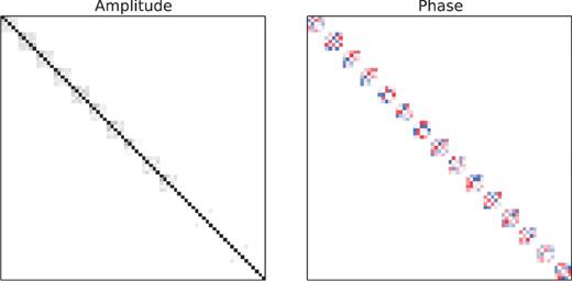
$Amplitude (left-hand panel) and phase (right-hand panel) of the block-diagonal matrix (${\bf J}$H${\bf J}$)UL for the data set described in the text. Each block corresponds to one antenna; the pixels within a block correspond to directions.$

Figure 2.

Amplitude (left-hand panel) and phase (right-hand panel) of the block-diagonal matrix (⁠|${\bf J}$|^H|${\bf J}$|⁠)_UL for the data set described in the text. Each block corresponds to one antenna; the pixels within a block correspond to directions.

Open in new tab Download slide

Figure 3.

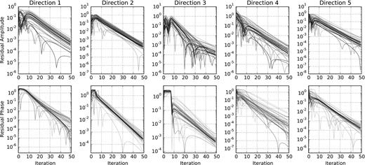
Amplitude (top row) and phase (bottom row) of the difference between the estimated and true gains, as a function of iteration. Columns correspond to directions. Different lines correspond to different antennas.

Open in new tab Download slide

7.2.2 Time-variable DD gains

To simulate a more realistic data set, we use a sky model composed of 100 point sources of random (uniformly distributed) flux density. We also add noise to the visibilities, at a level of about 1 per cent of the total flux. We simulate (scalar, phase-only) DD gains, using an ionospheric model consisting of a simple phase screen (an infinitesimally thin layer at a height of 100 km). The total electron content (TEC) values at the set of sample points are generated using Karhunen–Loeve decomposition (the spatial correlation is given by Kolmogorov turbulence; see van der Tol 2009). The constructed TEC screen has an amplitude of ∼0.07 TEC-Unit, and the corresponding DD phase terms are plotted in Fig. 4.

For calibration purposes, the sources are clustered in 10 directions using Voronoi tessellation (Fig. 5). The solution time interval is set to 4 min, and a separate gain solution is obtained per each direction. Fig. 6 shows images generated from the residual visibilities, where the best-fitting model is subtracted in the visibility domain. The rms residuals after CohJones has been applied are a factor of ∼4 lower than without DD solutions.

Figure 4.

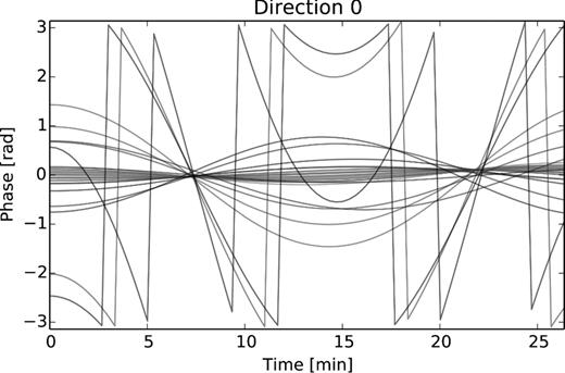
The complex phases of the DD gain terms (for all antennas and a single direction) derived from the time-variable TEC screen used in Section 7.2.2.

Open in new tab Download slide

Figure 5.

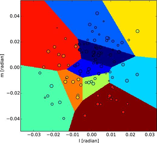
In order to conduct DD calibration, sources are clustered using a Voronoi tessellation algorithm. Each cluster has its own DD gain solution.

Open in new tab Download slide

Figure 6.

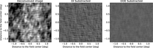
Simulation with time-variable DD gains. We show a deconvolved image (left) where no DD solutions have been applied, a residual image (centre) made by subtracting the sky model (in the visibility plane) without any DD corrections, and a residual image (right) made by subtracting the sky model with CohJones estimated DD gain solutions (right). The colour scale is the same in all panels. In this simulation, applying CohJones for DD calibration reduces the residual rms level by a factor of ∼4.

Open in new tab Download slide

8 CONCLUSIONS

Recent developments in optimization theory have extended traditional NLLS optimization approaches to functions of complex variables. We have applied this to radio interferometric gain calibration, and shown that the use of complex Jacobians allows for new insights into the problem, leading to the formulation of a whole new family of DI and DD calibration algorithms. These algorithms hinge around different sparse approximations of the |${\bf J}$|^H|${\bf J}$| matrix; we show that some recent algorithmic developments, notably StefCal, naturally fit into this framework as a particular special case of sparse (specifically, diagonal) approximation.

The proposed algorithms have different scaling properties depending on the selected matrix approximation – in all cases better than the cubic scaling of brute-force GN or LM methods – and may therefore exhibit different computational advantages depending on the dimensionality of the problem (number of antennas, number of directions). We also demonstrate an implementation of one particular algorithm for DD gain calibration, CohJones.

The use of complex Jacobians results in relatively compact and simple equations, and the resulting algorithms tend to be embarrassingly parallel, which makes them particularly amenable to implementation on new massively parallel computing architectures such as GPUs.

Complex optimization is applicable to a broader range of problems. Solving for a large number of independent DD gain parameters is not always desirable, as it potentially makes the problem underconstrained, and can lead to artefacts such as ghosts and source suppression. The alternative is solving for DD effect models that employ (a smaller set of) physical parameters, such as parameters of the primary beam and ionosphere. If these parameters are complex, then the complex Jacobian approach applies. Finally, although this paper only treats the NLLS problem (thus implicitly assuming Gaussian statistics), the approach is valid for the general optimization problem as well.

Other approximations or fast ways of inverting the complex |${\bf J}$|^H|${\bf J}$| matrix may exist, and future work can potentially yield new and faster algorithms within the same unifying mathematical framework. This flexibility is particularly important for addressing the computational needs of the new generation of the so-called ‘Square Kilometre Array (SKA) pathfinder’ telescopes, as well as the SKA itself.

We would like to thank the referee, Johan Hamaker, for extremely valuable comments that improved the paper. This work is based upon research supported by the South African Research Chairs Initiative of the Department of Science and Technology and National Research Foundation. Trienko Grobler originally pointed us in the direction of Wirtinger derivatives.

1

It should be stressed that Wirtinger calculus can be applied to a broader range of optimization problems than just LS.

2

Laurent et al. (2012) define the Jacobian via |$\mathrm{\partial} \boldsymbol {r}$| rather than |$\mathrm{\partial} \boldsymbol {v}$|⁠. This yields a Jacobian of the opposite sign, and introduces a minus sign into equations (2.8) and (2.9). In this paper we use the |$\mathrm{\partial} \boldsymbol {v}$| convention, as is more common in the context of radio interferometric calibration.

3

In principle, the autocorrelation terms pp, corresponding to the total power in the field, are also measured, and may be incorporated into the equations here. It is, however, common practice to omit autocorrelations from the interferometric calibration problem due to their much higher noise, as well as technical difficulties in modelling the total intensity contribution. The derivations below are equally valid for p ≤ q; we use p < q for consistency with practice.

4

In fact it was the initial development of CohJones by Tasse (2014b) that directly led to the present work.

5

The term ‘peeling’ has occasionally been misappropriated to describe other schemes, e.g. simultaneous independent DD gain solutions. We consider this a misuse: both the original formulation by Noordam (2004) and the word ‘peeling’ itself strongly imply dealing with one direction at a time.

6

https://code.google.com/p/pyrap

7

https://code.google.com/p/casacore

8

Note that Hamaker (2000) employs a similar formalism, but uses the (non-canonical) stacked rows definition instead.

9

see below

REFERENCES

Hamaker

J. P.

,

A&AS

,

2000

, vol.

143

pg.

515

Crossref

Search ADS

Hamaker

J. P.

Bregman

J. D.

Sault

R. J.

,

A&AS

,

1996

, vol.

117

pg.

137

Crossref

Search ADS

Kazemi

S.

Yatawatta

S.

,

MNRAS

,

2013

, vol.

435

pg.

597

Crossref

Search ADS

Kreutz-Delgado

K.

,

2009

preprint (arXiv:0906.4835)

Laurent

S.

van Barel

M.

de Lathauwer

L.

,

SIAM J. Optimization

,

2012

, vol.

22

pg.

879

Crossref

Search ADS

Madsen

K.

Nielsen

H. B.

Tingleff

O.

,

Methods For Non-linear Least Squares Problems. Informatics and Mathematical Modelling

,

2004

Lyngby

Technical University of Denmark

Google Scholar

Google Preview

OpenURL Placeholder Text

WorldCat

Mitchell

D. A.

Greenhill

L. J.

Wayth

R. B.

Sault

R. J.

Lonsdale

C. J.

Cappallo

R. J.

Morales

M. F.

Ord

S. M.

,

IEEE J. Selected Topics Signal Processing

,

2008

, vol.

2

pg.

707

Crossref

Search ADS

Noordam

J. E.

Oschmann

J. M.

Jr

,

Proc. SPIE, Vol. 5489, Ground-Based Telescopes

,

2004

Bellingham

SPIE

pg.

817

Google Scholar

Google Preview

OpenURL Placeholder Text

WorldCat

Noordam

J. E.

Smirnov

O. M.

,

A&A

,

2010

, vol.

524

pg.

A61

Crossref

Search ADS

Perley

R.

,

High Dynamic Range Imaging. Presentation at The Radio Universe @ Ger's (Wave)-length Conference

,

2013

Groningen (http://www.astron.nl/gerfeest/presentations/perley.pdf)

Google Scholar

Google Preview

OpenURL Placeholder Text

WorldCat

Salvini

S.

Wijnholds

S. J.

,

A&A

,

2014a

, vol.

571

pg.

A97

Crossref

Search ADS

Salvini

S.

Wijnholds

S. J.

,

General Assembly and Scientific Symposium (URSI GASS), 2014 XXXIth URSI

,

2014b

pg.

1

StEFCal–An Alternating Direction Implicit method for fast full polarization array calibration

Google Scholar

Google Preview

OpenURL Placeholder Text

WorldCat

Smirnov

O. M.

,

A&A

,

2011a

, vol.

527

pg.

A106

Crossref

Search ADS

Smirnov

O. M.

,

A&A

,

2011b

, vol.

527

pg.

A107

Crossref

Search ADS

Smirnov

O. M.

,

A&A

,

2011c

, vol.

527

pg.

A108

Crossref

Search ADS

Smirnov

O. M.

,

StefCal: The Fastest Selfcal in the West

,

2013

Presentation at 3GC3 Workshop, Port Alfred (http://tinyurl.com/pzu8hco)

Google Scholar

Google Preview

OpenURL Placeholder Text

WorldCat

Tasse

C.

,

A&A

,

2014a

, vol.

566

pg.

A127

Crossref

Search ADS

Tasse

C.

,

2014b

preprint (arXiv:410.8706)

van der Tol

S.

,

PhD thesis

,

2009

TU Delft

Google Scholar

Google Preview

OpenURL Placeholder Text

WorldCat

Wirtinger

W.

,

Math. Ann.

,

1927

, vol.

97

pg.

357

Crossref

Search ADS

APPENDIX A: |${\bf J}$| AND |$\boldsymbol {{{\bf J}}^{\rm H}{{\bf J}}}$| FOR THE THREE-ANTENNA CASE

To give a specific example of complex Jacobians, consider the three-antenna case. Using the numbering convention for pq of 12, 13, 32, we obtain the following partial Jacobians (equations 3.4 and 3.5):

\begin{eqnarray} {{\bf J}}_k = \left[\begin{array}{@{}ccc@{}}m_{12}\bar{g}_2 &\quad 0 &\quad 0 \nonumber\\ m_{13}\bar{g}_3 &\quad 0 &\quad 0 \nonumber\\ 0 &\quad m_{23}\bar{g}_3 &\quad 0 \end{array} \right],\quad {{\bf J}}_{k^*} = \left[\begin{array}{@{}ccc@{}}0 &\quad g_1 m_{12} &\quad 0 \nonumber\\ 0 &\quad 0 &\quad g_1 m_{13} \nonumber\\ 0 &\quad 0 &\quad g_2 m_{23} \end{array} \right].\nonumber\\ \end{eqnarray}

(A1)

We then get the following expression for the full complex Jacobian |${\bf J}$| (equation 3.8):

\begin{equation} \left[\begin{array}{@{}cccccc@{}} m_{12}\bar{g}_2 &\quad 0 &\quad 0 &\quad 0 &\quad g_1 m_{12} &\quad 0 \\ m_{13}\bar{g}_3 &\quad 0 &\quad 0 &\quad 0 &\quad 0 &\quad g_1 m_{13} \\ 0 &\quad m_{21}\bar{g}_1 &\quad 0 &\quad g_2 m_{21} &\quad 0 &\quad 0 \\ 0 &\quad m_{23}\bar{g}_3 &\quad 0 &\quad 0 &\quad 0 &\quad g_2 m_{23} \\ 0 &\quad 0 &\quad m_{31}\bar{g}_1 &\quad g_1 m_{31} &\quad 0 &\quad 0 \\ 0 &\quad 0 &\quad m_{32}\bar{g}_2 &\quad 0 &\quad g_3 m_{32} &\quad 0 \\ \end{array} \right]. \end{equation}

(A2)

Then, with the usual shorthand of |$y_{pq} = m_{pq} \bar{g}_q$|⁠, the |${\bf J}$|^H|${\bf J}$| term becomes

\begin{equation} \left[\begin{array}{@{}@{\ }c@{}c@{}c@{}c@{}c@{}c@{\ }@{}}\scriptstyle {y^2_{12}+y^2_{13}} &\quad\scriptstyle 0 &\quad\scriptstyle 0 &\quad\scriptstyle 0 &\quad\scriptstyle {\bar{y}_{12}\bar{y}_{21}} &\quad\scriptstyle {\bar{y}_{13}\bar{y}_{31}} \\ \scriptstyle 0 &\quad\scriptstyle {y^2_{12}+y^2_{23}} &\quad\scriptstyle 0 &\quad\scriptstyle {\bar{y}_{12}\bar{y}_{21}} &\quad\scriptstyle 0 &\quad\scriptstyle {\bar{y}_{23}\bar{y}_{32}} \\ \scriptstyle 0 &\quad\scriptstyle 0 &\quad\scriptstyle {y^2_{13}+y^2_{23}} &\quad\scriptstyle {\bar{y}_{13}\bar{y}_{31}} &\quad\scriptstyle {\bar{y}_{23}\bar{y}_{32}} &\quad\scriptstyle 0 \\ \scriptstyle 0 &\quad\scriptstyle y_{12}y_{21} &\quad\scriptstyle y_{13}y_{31} &\quad\scriptstyle {y^2_{12}+y^2_{13}} &\quad\scriptstyle 0 &\quad\scriptstyle 0 \\ \scriptstyle y_{12}y_{21} &\quad\scriptstyle 0 &\quad\scriptstyle y_{23}y_{32} &\quad\scriptstyle 0 &\quad\scriptstyle {y^2_{12}+y^2_{23}} &\quad\scriptstyle 0 \\ \scriptstyle y_{13}y_{31} &\quad\scriptstyle y_{23}y_{32} &\quad\scriptstyle 0 &\quad\scriptstyle 0 &\quad\scriptstyle 0 &\quad\scriptstyle {y^2_{13}+y^2_{23}} \\ \end{array} \right]. \end{equation}

(A3)

Finally, the three-antenna |${{\bf J}}^{\rm H}\boldsymbol {\breve{r}}$| term becomes

\begin{equation} {{\bf J}}^{\rm H}\boldsymbol {\breve{r}}= \left[\begin{array}{@{}c@{}} \bar{y}_{12} r_{12} + \bar{y}_{13} r_{13} \\ \bar{y}_{21} r_{21} + \bar{y}_{23} r_{23} \\ \bar{y}_{31} r_{31} + \bar{y}_{32} r_{32} \\ y_{12} \bar{r}_{12} + y_{13} \bar{r}_{13} \\ y_{21} \bar{r}_{21} + y_{23} \bar{r}_{23} \\ y_{31} \bar{r}_{31} + y_{32} \bar{r}_{32} \\ \end{array} \right]. \end{equation}

(A4)

APPENDIX B: Operator calculus

First, let us introduce the vectorization operator ‘vec’ and its inverse in the usual (stacked columns) way.⁸ For a 2 × 2 matrix |${\bf X}$|⁠:

\begin{equation} \mathrm{vec}\,{{{\bf X}}} = \left[\begin{array}{@{}c@{}}x_{11}\\ x_{21}\\ x_{12}\\ x_{22}\end{array} \right],\ \quad \ \mathrm{vec}^{-1}\,{\left[\begin{array}{@{}c@{}}x_{11}\\ x_{21}\\ x_{12}\\ x_{22}\end{array} \right]} = {{\bf X}}, \end{equation}

(B1)

which sets up an isomorphism between the space of 2 × 2 complex matrices |$\mathbb {C}^{2\times 2}$| and the space of 4-vectors |$\mathbb {C}^4$|⁠. Note that the ‘vec’ operator is linear, in other words the isomorphism preserves linear structure:

\begin{equation} \mathrm{vec}\,{({{\bf X}}+a{{\bf Y}})}=\mathrm{vec}\,{{{\bf X}}}+a\,\mathrm{vec}\,{{{\bf Y}}}, \end{equation}

(B2)

as well as the Frobenius norm:

\begin{equation} \Vert \mathrm{vec}\,{{{\bf X}}}\Vert _{\rm F} = \Vert {{\bf X}}\Vert _{\rm F}. \end{equation}

(B3)

Consider now the set of all linear operators on |$\mathbb {C}^{2\times 2}$|⁠, or |$\mathrm{Lin}(\mathbb {C}^{2\times 2},\mathbb {C}^{2\times 2}).$| Any such linear operator |$\mathcal {B}$|⁠, whose action we will write as |$\mathcal {B}{{\bf X}}$|⁠, can be associated with a linear operator on a 4-vector |${{\bf B}}\in \mathrm{Lin}(\mathbb {C}^4,\mathbb {C}^4)$|⁠, by defining |${\bf B}$| as

\begin{equation} {{\bf B}}\boldsymbol {x} = \mathrm{vec}\,{\mathcal {B}{{\bf X}}},\ \ \ {{\bf X}}=\mathrm{vec}^{-1}\,{\boldsymbol {x}}. \end{equation}

(B4)

Conversely, any linear operator on 4-vectors |${\bf B}$| can be associated with a linear operator on 2 × 2 matrices by defining

\begin{equation} \mathcal {B}{{\bf X}} = \mathrm{vec}^{-1}\,{{{\bf B}}\boldsymbol {x}},\ \ \ \boldsymbol {x}=\mathrm{vec}\,{{{\bf X}}}. \end{equation}

(B5)

Now, the set |$\mathrm{Lin}(\mathbb {C}^4,\mathbb {C}^4)$| is simply the set of all 4 × 4 matrix multipliers. Equations (B5) and (B5) establish a one-to-one mapping between this set and the set of linear operators on 2 × 2 matrices. In other words, the ‘vec’ operator induces two isomorphisms: one between |$\mathbb {C}^4$| and |$\mathbb {C}^{2\times 2}$|⁠, and the other between |$\mathbb {C}^{4\times 4}$| and linear operators on |$\mathbb {C}^{2\times 2}$|⁠. We will designate the second isomorphism by the symbol |$\mathbb {W}$|⁠:

\begin{equation} \begin{array}{ll} \mathbb {W}\mathcal {B} = {{\bf B}}: &\quad {{\bf B}}\boldsymbol {x} = \mathrm{vec}\,{\,(\mathcal {B}\,\mathrm{vec}^{-1}\,{\boldsymbol {x}}}), \\ \mathbb {W}^{-1}{{\bf B}} = \mathcal {B}: &\quad \mathcal {B}{{\bf X}} = \mathrm{vec}^{-1}\,{({{\bf B}}\,\mathrm{vec}\,{{{\bf X}}})}. \end{array} \end{equation}

(B6)

Note that |$\mathbb {W}$| also preserves linear structure.

Of particular interest to us are two linear operators on |$\mathbb {C}^{2\times 2}$|⁠: right-multiply by some 2 × 2 complex matrix |${\bf A}$|⁠, and left-multiply by |${\bf A}$|⁠:

\begin{equation} \mathcal {R}_{{{{\bf A}}}}{{\bf X}} = {{\bf XA}}, \ \ \ \mathcal {L}_{{{{\bf A}}}}{{\bf X}} = {{\bf AX}}. \end{equation}

(B7)

The |$\mathbb {W}$| isomorphism ensures that these operators can be represented as multiplication of 4-vectors by specific kinds of 4 × 4 matrices. The matrix outer product proves to be useful here, and in particular the following basic relation:

\begin{equation} \mathrm{vec}\,{(}{{\bf A}}{{\bf B}}{{\bf C}}) = ({{\bf C}}^{\rm T} \otimes {{\bf A}})\,\mathrm{vec}\,{{{\bf B}}}, \end{equation}

(B8)

from which we can derive the matrix operator forms via

\begin{equation} \begin{array}{l}\mathrm{vec}\,{(}\mathbb {I}{{\bf X}}{{\bf A}}) = ({{\bf A}}^{\rm T} \otimes \mathbb {I})\,\mathrm{vec}\,{{{\bf X}}},\\ \mathrm{vec}\,{(}{{\bf A}}{{\bf X}}\mathbb {I}) = (\mathbb {I}\otimes {{\bf A}})\,\mathrm{vec}\,{{{\bf X}}}, \end{array} \end{equation}

(B9)

which give us

\begin{equation} \mathbb {W}\mathcal {R}_{{{{\bf A}}}} = \left[\begin{array}{@{}c@{\quad}c@{\quad}c@{\quad}c@{}}a_{11}&\quad0&\quad a_{21}&\quad0 \\ 0&\quad a_{11}&\quad0&\quad a_{21} \\ a_{12}&\quad0&\quad a_{22}&\quad0 \\ 0&\quad a_{12}&\quad0&\quad a_{22} \end{array} \right] \end{equation}

(B10)

and

\begin{equation} \mathbb {W}\mathcal {L}_{{{{\bf A}}}} = \left[\begin{array}{@{}c@{\quad}c@{\quad}c@{\quad}c@{}}a_{11}&\quad a_{12}&\quad0&\quad0 \\ a_{21}&\quad a_{22}&\quad0&\quad0 \\ 0&\quad0&\quad a_{11}&\quad a_{12} \\ 0&\quad0&\quad a_{21}&\quad a_{22} \end{array} \right]. \end{equation}

(B11)

From this we get the important property that

\begin{equation} [\mathbb {W}\mathcal {R}_{{{{\bf A}}}}]^{\rm H} = \mathbb {W}\mathcal {R}_{{{{\bf A}}^{\rm H}}},\ \ \ [\mathbb {W}\mathcal {L}_{{{{\bf A}}}}]^{\rm H} = \mathbb {W}\mathcal {L}_{{{{\bf A}}^{\rm H}}}. \end{equation}

(B12)

Note that equation (5.5), which we earlier derived from the operator definitions, can now be verified with the 4 × 4 forms. Note also that equation (5.5) is equally valid whether interpreted in terms of chaining operators, or multiplying the equivalent 4 × 4 matrices.

B1 Derivative operators and Jacobians

Consider a matrix-valued function of a matrix argument and its Hermitian transpose, |${\bf F}$|(⁠|${\bf G}$|⁠, |${\bf G}$|^H). Yet again, we can employ the ‘vec’ operator to construct a one-to-one mapping between such functions and 4-vector valued functions of 4-vectors:

\begin{equation} \boldsymbol {f}(\boldsymbol {g},\boldsymbol {\bar{g}}) = \mathrm{vec}\,{{{\bf F}}(\mathrm{vec}^{-1}\,{\boldsymbol {g}},(\mathrm{vec}^{-1}\,{\boldsymbol {\bar{g}}})^{\rm T})}. \end{equation}

(B13)

Consider now the partial and conjugate partial Jacobians of |$\boldsymbol {f}$| with respect to |$\boldsymbol {g}$| and |$\bar{\boldsymbol {g}}$|⁠, defined as per the formalism of Section 2. These are 4 × 4 matrices, as given by equation (3.4),

\begin{equation} {{\bf J}}_k = [ \mathrm{\partial} f_i / \mathrm{\partial} g_j ],\ \ \ {{\bf J}}_{k^*} = [ \mathrm{\partial} f_i / \mathrm{\partial} \bar{g}_j ], \end{equation}

(B14)

that represent local linear approximations to |$\boldsymbol {f}$|⁠, i.e. linear operators on |$\mathbb {C}^4$| that map increments in the arguments |$\Delta \boldsymbol {g}$| and |$\Delta \boldsymbol {\bar{g}}$| to increments in the function value |$\Delta \boldsymbol {f}$|⁠. The |$\mathbb {W}$| isomorphism defined above matches these operators to linear operators on |$\mathbb {C}^{2\times 2}$| that represent linear approximations to |$\boldsymbol {F}$|⁠. It is the latter operators that we shall call the Wirtinger matrix derivatives of |${\bf F}$| with respect to |${\bf G}$| and |${\bf G}$|^H:

\begin{equation} \frac{\mathrm{\partial} {{\bf F}}}{\mathrm{\partial} {{{\bf G}}}} = \mathbb {W}^{-1}({{\bf J}}_k),\ \ \ \frac{\mathrm{\partial} {{\bf F}}}{\mathrm{\partial} {{{\bf G}}^{\rm H}}} = \mathbb {W}^{-1}({{\bf J}}_{k^*}^{\rm T}). \end{equation}

(B15)

This is more than just a formal definition: thanks to the |$\mathbb {W}$| isomorphism, the operators given by equation (B15) are Wirtinger derivatives in exactly the same sense that the Jacobians of equation (B14) are Wirtinger derivatives, with the former being simply the |$\mathbb {C}^{2\times 2}$| manifestation of the gradient operators in |$\mathbb {C}^4$|⁠, as defined in Section 2. However, operating in |$\mathbb {C}^{2\times 2}$| space allows us to write the larger Jacobians of Section 5 in terms of simpler matrices composed of operators, resulting in a Jacobian structure that is entirely analogous to the scalar derivation.

APPENDIX C: GRADIENT-BASED OPTIMIZATION ALGORITHMS

This appendix documents the various standard least-squares optimization algorithms that are referenced in this paper.

C1 Algorithm SD (steepest descent)

Start with a best guess for the parameter vector, |$\boldsymbol {z}_0$|⁠;
at each step k, compute the residuals |$\boldsymbol {\breve{r}}_k$|⁠, and the Jacobian |${{\bf J}}={{\bf J}}(\boldsymbol {\breve{z}}_k)$|⁠;
compute the parameter update as (note that due to redundancy, only the top half of the vector actually needs to be computed):
\begin{equation} \delta \boldsymbol {\breve{z}}_k = - \lambda {{\bf J}}^{\rm H} \boldsymbol {\breve{r}}_k, \end{equation}
(C1)
where λ is some small value;
if not converged,⁹ set |$\boldsymbol {z}_{k+1}=\boldsymbol {z}_k+\delta \boldsymbol {z}$|⁠, and go back to step (ii).

C2 Algorithm GN

Start with a best guess for the parameter vector, |$\boldsymbol {z}_0$|⁠;
at each step k, compute the residuals |$\boldsymbol {\breve{r}}_k$|⁠, and the Jacobian |${{\bf J}}={{\bf J}}(\boldsymbol {\breve{z}}_k)$|⁠;
compute the parameter update |$\delta \boldsymbol {\breve{z}}$| using equation (2.9) with λ = 0 (note that only the top half of the vector actually needs to be computed);
if not converged, set |$\boldsymbol {z}_{k+1}=\boldsymbol {z}_k+\delta \boldsymbol {z}$|⁠, and go back to step (ii).

C3 Algorithm LM

Several variations of this exist, but a typical one is

start with a best guess for the parameter vector, |$\boldsymbol {z}_0$|⁠, and an initial value for the damping parameter, e.g. λ = 1;
at each step k, compute the residuals |$\boldsymbol {\breve{r}}_k$|⁠, and the cost function |$\chi ^2_k=\Vert \boldsymbol {\breve{r}}_k\Vert _{\rm F}$|⁠;
if |$\chi ^2_k\ge \chi ^2_{k-1}$| (unsuccessful step), reset |$\boldsymbol {z}_k=\boldsymbol {z}_{k-1}$|⁠, and set λ = λK (where typically K = 10);
otherwise (successful step) set λ = λ/K;
compute the Jacobian |${{\bf J}}={{\bf J}}(\boldsymbol {\breve{z}}_k)$|⁠;
compute the parameter update |$\delta \boldsymbol {\breve{z}}_k$| using equation (2.9) (note that only the top half of the vector actually needs to be computed);
if not converged, set |$\boldsymbol {z}_{k+1}=\boldsymbol {z}_k+\delta \boldsymbol {z}$|⁠, and go back to step (ii).

C4 Convergence

All of the above algortihms iterate to ‘convergence’. One or more of the following convergence criteria may be implemented in each case.

Parameter update smaller than some pre-defined threshold: |$\Vert \delta \boldsymbol {z}\Vert _{\rm F}<\delta _0$|⁠.
Improvement to cost function smaller than some pre-defined threshold: |$\chi ^2_{k-1}-\chi ^2_{k}<\epsilon _0$|⁠.
Norm of the gradient smaller than some threshold: |||${\bf J}$|||_F < γ₀.

Download all slides

Month:	Total Views:
January 2017	3
February 2017	14
March 2017	6
April 2017	7
May 2017	2
June 2017	3
July 2017	9
August 2017	1
September 2017	11
October 2017	8
November 2017	4
December 2017	4
January 2018	3
February 2018	2
March 2018	4
April 2018	3
May 2018	6
June 2018	9
July 2018	15
August 2018	14
September 2018	5
October 2018	13
November 2018	8
December 2018	3
January 2019	9
February 2019	24
March 2019	17
April 2019	15
May 2019	17
June 2019	13
July 2019	12
August 2019	14
September 2019	12
October 2019	28
November 2019	20
December 2019	11
January 2020	9
February 2020	11
March 2020	23
April 2020	15
May 2020	14
June 2020	13
July 2020	9
August 2020	7
September 2020	12
October 2020	9
November 2020	14
December 2020	16
January 2021	10
February 2021	23
March 2021	30
April 2021	18
May 2021	7
June 2021	23
July 2021	16
August 2021	8
September 2021	9
October 2021	20
November 2021	13
December 2021	24
January 2022	27
February 2022	20
March 2022	31
April 2022	11
May 2022	21
June 2022	12
July 2022	15
August 2022	9
September 2022	20
October 2022	22
November 2022	17
December 2022	17
January 2023	18
February 2023	10
March 2023	18
April 2023	24
May 2023	17
June 2023	19
July 2023	12
August 2023	29
September 2023	23
October 2023	41
November 2023	34
December 2023	24
January 2024	35
February 2024	24
March 2024	41
April 2024	37
May 2024	48
June 2024	26
July 2024	34
August 2024	14
September 2024	48
October 2024	46
November 2024	33
December 2024	20
January 2025	19
February 2025	20
March 2025	44
April 2025	24
May 2025	20

Article Contents

Radio interferometric gain calibration as a complex optimization problem Free

Abstract

1 INTRODUCTION

2 WIRTINGER CALCULUS AND COMPLEX LEAST SQUARES

3 SCALAR (UNPOLARIZED) CALIBRATION

3.1 Direction-independent calibration

3.2 Computing the parameter update

3.3 Time/frequency solution intervals

3.4 Weighting

3.5 Direction-dependent calibration

4 INVERTING |$\boldsymbol {{{\bf J}}^{\rm H}{{\bf J}}}$| AND SEPARABILITY

4.1 Diagonal approximation and StefCal

4.2 Separability of the direction-dependent case

4.2.1 DCA: separating by direction

4.2.2 COHJONES: separating by antenna

4.2.3 ALLJONES: separating all

4.3 Convergence and algorithmic cost

4.4 Smoothing in time and frequency

5 THE FULLY POLARIZED CASE

5.1 Matrix operators and derivatives

5.2 Complex Jacobians for the polarized RIME

5.3 Parameter updates and the diagonal approximation

5.4 Polarized direction-dependent calibration

6 OTHER DD ALGORITHMIC VARIATIONS

6.1 Feed-forward

6.2 Triangular approximation

6.3 Peeling

6.4 Exact matrix inversion

7 IMPLEMENTATIONS

7.1 StefCal in MeqTrees

7.2 CohJones tests with simulated data

7.2.1 Constant DD gains

7.2.2 Time-variable DD gains

8 CONCLUSIONS

REFERENCES

APPENDIX A: |${\bf J}$| AND |$\boldsymbol {{{\bf J}}^{\rm H}{{\bf J}}}$| FOR THE THREE-ANTENNA CASE

APPENDIX B: Operator calculus

B1 Derivative operators and Jacobians

APPENDIX C: GRADIENT-BASED OPTIMIZATION ALGORITHMS

C1 Algorithm SD (steepest descent)

C2 Algorithm GN

C3 Algorithm LM

C4 Convergence

Citations

Views

Altmetric

Email alerts

Astrophysics Data System

Citing articles via

Latest

Most Read

Most Cited

This Feature Is Available To Subscribers Only

Radio interferometric gain calibration as a complex optimization problem