


Abstract
In 2013 April a new magnetar, SGR 1745−2900, was discovered as it entered an outburst, at only 2.4 arcsec angular distance from the supermassive black hole at the centre of the Milky Way, Sagittarius A*. SGR 1745−2900 has a surface dipolar magnetic field of ∼2 × 10¹⁴ G, and it is the neutron star closest to a black hole ever observed. The new source was detected both in the radio and X-ray bands, with a peak X-ray luminosity LX ∼ 5 × 1035 erg s−1. Here we report on the long-term Chandra (25 observations) and XMM–Newton (eight observations) X-ray monitoring campaign of SGR 1745−2900 from the onset of the outburst in 2013 April until 2014 September. This unprecedented data set allows us to refine the timing properties of the source, as well as to study the outburst spectral evolution as a function of time and rotational phase. Our timing analysis confirms the increase in the spin period derivative by a factor of ∼2 around 2013 June, and reveals that a further increase occurred between 2013 October 30 and 2014 February 21. We find that the period derivative changed from 6.6 × 10⁻¹² to 3.3 × 10⁻¹¹ s s−1 in 1.5 yr. On the other hand, this magnetar shows a slow flux decay compared to other magnetars and a rather inefficient surface cooling. In particular, starquake-induced crustal cooling models alone have difficulty in explaining the high luminosity of the source for the first ∼200 d of its outburst, and additional heating of the star surface from currents flowing in a twisted magnetic bundle is probably playing an important role in the outburst evolution.
1 INTRODUCTION
Among the large variety of Galactic neutron stars, magnetars constitute the most unpredictable class (Mereghetti 2008; Rea & Esposito 2011). They are isolated X-ray pulsars rotating at relatively long periods (P ∼ 2–12 s, with spin period derivatives |$\dot{P}\sim 10^{-15}$|–10−10 s s−1), and their emission cannot be explained within the commonly accepted scenarios for rotation-powered pulsars. In fact, their X-ray luminosity (typically LX ∼ 1033–1035 erg s−1) generally exceeds the rotational energy loss rate and their temperatures are often higher than non-magnetic cooling models predict. It is now generally recognized that these sources are powered by the decay and the instability of their exceptionally high magnetic field (up to B ∼ 1014–1015 G at the star surface), hence the name ‘magnetars’ (Duncan & Thompson 1992; Thompson & Duncan 1993; Thompson, Lyutikov & Kulkarni 2002). Alternative scenarios such as accretion from a fossil disc surrounding the neutron star (Chatterjee, Hernquist & Narayan 2000; Alpar 2001) or Quark-Nova models (Ouyed, Leahy & Niebergal 2007a,b) have not been ruled out (see Turolla & Esposito 2013, for an overview).
The persistent soft X-ray spectrum usually comprises both a thermal (blackbody, kT ∼ 0.3–0.6 keV) and a non-thermal (power law, Γ ∼ 2–4) components. The former is thought to originate from the star surface, whereas the latter likely comes from the reprocessing of thermal photons in a twisted magnetosphere through resonant cyclotron scattering (Thompson et al. 2002; Nobili, Turolla & Zane 2008a,b; Rea et al. 2008; Zane et al. 2009).
In addition to their persistent X-ray emission, magnetars exhibit very peculiar bursts and flares (with luminosities reaching up to 1046 erg s−1 and lasting from milliseconds to several minutes), as well as large enhancements of the persistent flux (outbursts), which can last years. These events may be accompanied or triggered by deformations/fractures of the neutron star crust (‘stellar quakes’) and/or local/global rearrangements of the star magnetic field.
In the past decade, extensive study of magnetars in outburst has led to a number of unexpected discoveries which have changed our understanding of these objects. The detection of typical magnetar-like bursts and a powerful enhancement of the persistent emission unveiled the existence of three low magnetic field (B < 4 × 10¹³ G) magnetars (Rea et al. 2010, 2012, 2014; Scholz et al. 2012; Zhou et al. 2014). Recently, an absorption line at a phase-variable energy was discovered in the X-ray spectrum of the low-B magnetar SGR 0418+5729; this, if interpreted in terms of a proton cyclotron feature, provides a direct estimate of the magnetic field strength close to the neutron star surface (Tiengo et al. 2013). Finally, a sudden spin-down event, i.e. an antiglitch, was observed for the first time in a magnetar (Archibald et al. 2013).
The discovery of the magnetar SGR 1745−2900 dates back to 2013 April 24, when the Burst Alert Telescope (BAT) on board the Swift satellite detected a short hard X-ray burst at a position consistent with that of the supermassive black hole at the centre of the Milky Way, Sagittarius A* (hereafter Sgr A*). Follow-up observations with the Swift X-ray Telescope (XRT) enabled characterization of the 0.3–10 keV spectrum as an absorbed blackbody (with kT ∼ 1 keV), and estimate a luminosity of ∼3.9 × 1035 erg s−1 (for an assumed distance of 8.3 kpc; Kennea et al. 2013a). The following day, a 94.5-ks observation performed with the Nuclear Spectroscopic Telescope Array (NuSTAR) revealed 3.76 s pulsations from the XRT source (Mori et al. 2013). This measurement was subsequently confirmed by a 9.8-ks pointing on April 29 with the High Resolution Camera (HRC) onboard the Chandra satellite, which was able to single out the magnetar counterpart at only 2.4 ± 0.3 arcsec from Sgr A*, confirming that the new source was actually responsible for the X-ray brightening observed in the Sgr A* region (Rea et al. 2013b). Follow-up observations in the 1.4–20 GHz band revealed the radio counterpart of the source and detected pulsations at the X-ray period (e.g. Eatough et al. 2013a; Shannon & Johnston 2013). The SGR-like bursts, the X-ray spectrum, and the surface dipolar magnetic field inferred from the measured spin period and spin-down rate, Bp ∼ 2 × 10¹⁴ G, led to classify this source as a magnetar (Kennea et al. 2013; Mori et al. 2013; Rea et al. 2013b).
SGR 1745−2900 holds the record as the closest neutron star to a supermassive black hole detected to date. The dispersion measure DM = 1778 ± 3 cm−3 pc is also the highest ever measured for a radio pulsar and is consistent with a source located within 10 pc of the Galactic Centre. Furthermore, its neutral hydrogen column density |${N_{\rm H}}\sim 10^{23}$| cm−2 is characteristic of a location at the Galactic Centre (Baganoff et al. 2003). The angular separation of 2.4 ± 0.3 arcsec from Sgr A* corresponds to a minimum physical separation of 0.09 ± 0.02 pc (at a 95 per cent confidence level; Rea et al. 2013b) for an assumed distance of 8.3 kpc (see e.g. Genzel, Eisenhauer & Gillessen 2010). Recent observations of the radio counterpart with the Very Long Baseline Array (VLBA) succeeded in measuring its transverse velocity of 236 ± 11 km s−1 at position angle of 22° ± 2° east of north (Bower et al. 2015). If born within 1 pc of Sgr A*, the magnetar has a ∼90 per cent probability of being in a bound orbit around the black hole, according to the numerical simulations of Rea et al. (2013b).
SGR 1745−2900 has been monitored intensively in the X-ray and radio bands since its discovery. Three high-energy bursts were detected from a position consistent with that of the magnetar on 2013 June 7, August 5 by Swift/BAT, and on 2013 September 20 by the International Gamma-Ray Astrophysics Laboratory (INTEGRAL; Barthelmy, Cummings & Kennea 2013a; Barthelmy et al. 2013b; Kennea et al. 2013b, Kennea et al. 2013c; Mereghetti et al. 2013). Kaspi et al. (2014) reported timing and spectral analysis of NuSTAR and Swift/XRT data for the first ∼4 months of the magnetar activity (2013 April–August). Interestingly, an increase in the source spin-down rate by a factor of ∼2.6 was observed, possibly corresponding to the 2013 June burst. The source has been observed daily with Swift/XRT until 2014 October, and its 2–10 keV flux has decayed steadily during this time interval (Lynch et al. 2015).
Radio observations made possible a value of the rotational measure, RM = 66960 ± 50 rad m−2, which implies a lower limit of ∼8 mG for the strength of the magnetic field in the vicinity of Sgr A* (Eatough et al. 2013b). Observations with the Green Bank Telescope showed that the source experienced a period of relatively stable 8.7-GHz flux between 2013 August and 2014 January and then entered a state characterized by a higher and more variable flux, until 2014 July (Lynch et al. 2015).
In this paper we report on the X-ray long-term monitoring campaign of SGR 1745−2900 covering the first 1.5 yr of the outburst decay. In Section 2 we describe the Chandra and XMM–Newton observations and the data analysis. In Section 3 we discuss our results; conclusions follow in Section 4.
2 OBSERVATIONS AND DATA ANALYSIS
The Chandra X-ray Observatory observed SGR 1745−2900 twenty-six times between 2013 April 29 and 2014 August 30. The first observation was performed with the HRC to have the best spatial accuracy to localize the source in the crowded region of the Galactic Centre (Rea et al. 2013b). The remaining observations were performed with the Advanced CCD Imaging Spectrometer (ACIS; Garmire et al. 2003) set in faint timed-exposure imaging mode with a 1/8 subarray (time resolution of 0.4 s), and in three cases with the High Energy Transmission Grating (HETG; Canizares et al. 2005). The source was positioned on the back-illuminated S3 chip. Eight observations were carried out by the XMM–Newton satellite using the European Photon Imaging Camera (EPIC), with the pn (Strüder et al. 2001) and the two MOS (Turner et al. 2001) CCD cameras operated in full-frame window mode (time resolution of 73.4 ms and 2.6 s, respectively), with the medium optical blocking filter in front of them. A log of the X-ray observations is given in Table 1.
Log of Chandra/ACIS-S and XMM–Newton/EPIC observations. Exposure times for the XMM–Newton observations are reported for the pn, MOS1, and MOS2 detectors, respectively, and source net counts refer to the pn detector.
| Obs. ID | MJD | Start time (TT) | End time (TT) | Exposure time | Source net counts |
|---|---|---|---|---|---|
| (yyyy/mm/dd hh:mm:ss) | (yyyy/mm/dd hh:mm:ss) | (ks) | (× 103) | ||
| 14702a | 56424.55 | 2013/05/12 10:38:50 | 2013/05/12 15:35:56 | 13.7 | 7.4 |
| 15040b | 56437.63 | 2013/05/25 11:38:37 | 2013/05/25 18:50:50 | 23.8 | 3.5 |
| 14703a | 56447.48 | 2013/06/04 08:45:16 | 2013/06/04 14:29:15 | 16.8 | 7.6 |
| 15651b | 56448.99 | 2013/06/05 21:32:38 | 2013/06/06 01:50:11 | 13.8 | 1.9 |
| 15654b | 56452.25 | 2013/06/09 04:26:16 | 2013/06/09 07:38:28 | 9.0 | 1.2 |
| 14946a | 56475.41 | 2013/07/02 06:57:56 | 2013/07/02 12:46:18 | 18.2 | 7.1 |
| 15041 | 56500.36 | 2013/07/27 01:27:17 | 2013/07/27 15:53:25 | 45.4 | 15.7 |
| 15042 | 56516.25 | 2013/08/11 22:57:58 | 2013/08/12 13:07:47 | 45.7 | 14.4 |
| 0724210201c | 56535.19 | 2013/08/30 20:30:39 | 2013/08/31 12:28:26 | 55.6/57.2/57.2 | 39.7 |
| 14945 | 56535.55 | 2013/08/31 10:12:46 | 2013/08/31 16:28:32 | 18.2 | 5.3 |
| 0700980101c | 56545.37 | 2013/09/10 03:18:13 | 2013/09/10 14:15:07 | 35.7/37.3/37.3 | 24.9 |
| 15043 | 56549.30 | 2013/09/14 00:04:52 | 2013/09/14 14:19:20 | 45.4 | 12.5 |
| 14944 | 56555.42 | 2013/09/20 07:02:56 | 2013/09/20 13:18:10 | 18.2 | 5.0 |
| 0724210501c | 56558.15 | 2013/09/22 21:33:13 | 2013/09/23 09:26:52 | 41.0/42.6/42.5 | 26.5 |
| 15044 | 56570.01 | 2013/10/04 17:24:48 | 2013/10/05 07:01:03 | 42.7 | 10.9 |
| 14943 | 56582.78 | 2013/10/17 15:41:05 | 2013/10/17 21:43:58 | 18.2 | 4.5 |
| 14704 | 56588.62 | 2013/10/23 08:54:30 | 2013/10/23 20:43:44 | 36.3 | 8.7 |
| 15045 | 56593.91 | 2013/10/28 14:31:14 | 2013/10/29 05:01:24 | 45.4 | 10.6 |
| 16508 | 56709.77 | 2014/02/21 11:37:48 | 2014/02/22 01:25:55 | 43.4 | 6.8 |
| 16211 | 56730.71 | 2014/03/14 10:18:27 | 2014/03/14 23:45:34 | 41.8 | 6.2 |
| 0690441801c | 56750.72 | 2014/04/03 05:23:24 | 2014/04/04 05:07:01 | 83.5/85.2/85.1 | 34.3 |
| 16212 | 56751.40 | 2014/04/04 02:26:27 | 2014/04/04 16:49:26 | 45.4 | 6.2 |
| 16213 | 56775.41 | 2014/04/28 02:45:05 | 2014/04/28 17:13:57 | 45.0 | 5.8 |
| 16214 | 56797.31 | 2014/05/20 00:19:11 | 2014/05/20 14:49:18 | 45.4 | 5.4 |
| 16210 | 56811.24 | 2014/06/03 02:59:23 | 2014/06/03 08:40:34 | 17.0 | 1.9 |
| 16597 | 56842.98 | 2014/07/04 20:48:12 | 2014/07/05 02:21:32 | 16.5 | 1.6 |
| 16215 | 56855.22 | 2014/07/16 22:43:52 | 2014/07/17 11:49:38 | 41.5 | 3.8 |
| 16216 | 56871.43 | 2014/08/02 03:31:41 | 2014/08/02 17:09:53 | 42.7 | 3.6 |
| 16217 | 56899.43 | 2014/08/30 04:50:12 | 2014/08/30 15:45:44 | 34.5 | 2.8 |
| 0743630201c | 56900.02 | 2014/08/30 19:37:28 | 2014/08/31 05:02:43 | 32.0/33.6/33.6 | 9.2 |
| 0743630301c | 56901.02 | 2014/08/31 20:40:57 | 2014/09/01 04:09:34 | 25.0/26.6/26.6 | 7.8 |
| 0743630401c | 56927.94 | 2014/09/27 17:47:50 | 2014/09/28 03:05:37 | 25.7/32.8/32.8 | 7.7 |
| 0743630501c | 56929.12 | 2014/09/28 21:19:11 | 2014/09/29 08:21:11 | 37.8/39.4/39.4 | 11.7 |
Notes. aObservations already analysed by Rea et al. (2013b). An additional Chandra/HRC observation was carried out on 2013 April 29.
bChandra grating observations.
cXMM–Newton observations.
Chandra data were analysed following the standard analysis threads1 with the Chandra Interactive Analysis of Observations software package (ciao, version 4.6; Fruscione et al. 2006). XMM–Newton data were processed using the Science Analysis Software (sas,2 version 13.5.0). For both Chandra and XMM–Newton data, we adopted the most recent calibration files available at the time the data reduction and analysis were performed.
2.1 Timing analysis
We extracted all Chandra and XMM–Newton/EPIC-pn source counts using a 1.5- and 15-arcsec circles, respectively, centred on the source position. Background counts were extracted using a nearby circular region of the same size. We adopted the coordinates reported by Rea et al. (2013b), i.e. |$\rm RA = 17 ^h 45^m 40{.\!\!^{{\mathrm{s}}}}169$|, Dec. = −29°00′29|${^{\prime\prime}_{.}}$|84 (J2000.0), to convert the photon arrival times to Solar system barycentre reference frame. The effects of the proper motion relative to Sgr A* on the source position are negligible on the time-scales considered for our analysis (best-fitting parameters are 1.6 < μα < 3.0 and 5.7 < μδ < 6.1 mas yr−1 at a 95 per cent confidence level; Bower et al. 2015).
To determine a timing solution valid over the time interval covered by the Chandra and XMM–Newton observations (from 2013 April 29 to 2014 August 30; see Table 1), we first considered the timing solutions given by Rea et al. (2013b; using Chandra and Swift) and Kaspi et al. (2014; using NuSTAR and Swift). In the overlapping time interval, before 2013 June 14 (MJD 56457), both papers report a consistent timing solution (see first column in Table 2 and green solid line in the upper panel of Fig. 1). Kaspi et al. (2014) then added more observations covering the interval between 2013 June 14 and August 15 (MJD 56457–56519), and observed a |$\dot{P}$| roughly two times larger than the previous value (see Table 2). The uncertainties on the Kaspi et al. (2014) solution formally ensure unambiguous phase connection until 2013 November 11 (MJD 56607), allowing us to extend this phase-coherent analysis with the data reported here, and follow the evolution of the pulse phases between 2013 July 27 and October 28 (MJD 56500–56594; after which we have a gap in our data coverage of about 115 d; see Table 2).

Upper panel: temporal evolution of the spin frequency of SGR 1745−2900. The solution given by Rea et al. (2013b) is plotted as a green solid line. The blue and magenta solid lines show solutions A and B of this work, respectively. The blue dashed lines are the extrapolation of solution A over the time span of solution B. The black line represents the fit over the whole time interval covered by observations (see text), while the vertical dashed lines refer to the times of the SGR-like short bursts detected by Swift/BAT (on 2013 April 25, June 7, and August 5). Central panel: phase residuals with respect to solution A (labelled as ϕ(t)A), evaluated over the time validity interval MJD 56500.1–56594.1. Lower panel: phase residuals with respect to solution B (labelled as νB(t)), evaluated over the time validity interval MJD 56709.5–56929.
Timing solutions. Errors were evaluated at the 1σ confidence level, scaling the uncertainties by the value of the rms (|$\sqrt{\chi _\nu ^2}$|) of the respective fit to account for the presence of unfitted residuals.
| Solution | Rea et al. (2013b) | Kaspi et al. (2014) | This work (solution A) | This work (solution B) |
| Epoch T0 (MJD) | 56424.5509871 | 56513.0 | 56513.0 | 56710.0 |
| Validity range (MJD) | 56411.6–56475.3 | 56457–56519 | 56500.1–56594.1 | 56709.5–56929 |
| P(T0) (s) | 3.7635537(2) | 3.76363824(13) | 3.76363799(7) | 3.7639772(12) |
| |$\dot{P}(T_0)$| | 6.61(4) × 10−12 | 1.385(15) × 10−11 | 1.360(6) × 10−11 | 3.27(7) × 10−11 |
| |$\ddot{P}$| (s−1) | 4(3) × 10−19 | 3.9(6) × 10−19 | 3.7(2) × 10−19 | ( − 1.8 ± 0.8) × 10−19 |
| ν(T0) (Hz) | 0.265706368(14) | 0.265700350(9) | 0.26570037(5) | 0.26567642(9) |
| |$\dot{\nu }(T_0)$| (Hz s−1) | −4.67(3) × 10−13 | −9.77(10) × 10−13 | −9.60(4) × 10−13 | −2.31(5) × 10−12 |
| |$\ddot{\nu }$| (Hz s−2) | −3(2) × 10−20 | −2.7(4) × 10−20 | −2.6(1) × 10−20 | (1.3 ± 0.6) × 10−20 |
| rms residual | 0.15 s | 51 ms | 0.396 s | 1.0 μHz |
| |$\chi _\nu ^2$| (d.o.f.) | 0.85 (5) | 1.27 (41) | 6.14 (44) | 0.66 (10) |
In this time interval, we measured the pulse phase at the fundamental frequency by dividing our observations in intervals of 10 ks and using the solution given by Kaspi et al. (2014) to determine univocally the number of cycles between the various observations. By fitting the measured pulse phases with a cubic function, we obtained the solution dubbed A in Table 2, which shows only slight deviations with respect to the solution published by Kaspi et al. (2014), but extends until 2013 October 28 (MJD 56594). The period evolution implied by solution A is plotted with a blue solid line in the upper panel of Fig. 1. Our Chandra and XMM–Newton observations allow us to confirm the change in the |$\dot{P}$|, which increased by a factor of ∼2 around 2013 June (i.e. about 2 months after the onset of the outburst in 2013 April), and remained stable until at least 2013 October 28.
Formally, the accuracy of solution A should guarantee that phase coherence is not lost before 2014 March 3 (MJD 56721), i.e. comprising the first observation available after the 115 d gap between MJD 56594.1 and MJD 56709.5. However, fitting the phases derived for that observation with solution A shows large residuals. These clearly indicate that solution A is not valid after the gap. To investigate this change in the spin evolution of the source, we measured the spin frequency for all the observations performed after the gap by fitting with a linear function the phases determined over time intervals with lengths ranging from 2 to 10 ks, depending on the source flux. The values for the frequencies we measured in this way after 2014 February 21 (MJD 56709) are much smaller than those predicted by solution A (see blue dashed line in the upper panel of Fig. 1).
To determine the spin evolution of the source after the 115 d gap in the observations (i.e. from MJD 56709), we then fitted the values of the spin frequency with a quadratic function, obtaining the non-coherent solution B (see Table 2), plotted in the upper panel of Fig. 1 with a magenta solid line. Unfortunately, this solution is not accurate enough to determine univocally the number of rotations between the various observations. Still, the trend followed by the spin frequency after the gap clearly deviates from that shown before 2013 October 28 via solution A, indicating a further increase of the spin-down rate. In particular, the |$\dot{P}$| has further increased by a factor of ∼2.5, and the |$\ddot{P}$| is smaller than that measured by solution A, even if the large error prevents us from detecting a change in the sign of the |$\ddot{P}$| at high significance.
The large changes in the timing properties of the source since the onset of the outburst are also shown by the fact that a quadratic function gives a poor fit for the spin frequency evolution over the whole time interval covered by the observations [|$\chi ^2_\nu =5.04$| for 26 degrees of freedom (d.o.f.); see black solid line in the upper panel of Fig. 1].
Summarizing, we derive a phase coherent solution (solution A, see Table 2 and blue solid line in the upper panel of Fig. 1) that is able to model the pulse phase evolution before the 115 d observations gap starting at MJD 56600, and which is compatible with the solution given by Kaspi et al. (2014) for the partly overlapping interval MJD 56457–56519. After the observation gap, solution A is no longer able to provide a good description of pulse phases, and we are only able to find a solution based on the analysis of the spin frequency evolution (solution B, see Table 2 and magenta solid line in the upper panel of Fig. 1).
We then use timing solution A (up to MJD 56594.1) and solution B (from MJD 56709.5 onwards) to fold all background-subtracted and exposure-corrected light curves at the neutron star spin period during the corresponding observation. This allows us to extract the temporal evolution of the pulsed fraction, defined as PF = [Max-Min]/[Max + Min] (Max and Min being the maximum and the minimum count rate of the pulse profile, respectively). To investigate possible dependences on energy, we calculate the pulsed fractions in the 0.3–3.5 and 3.5–10 keV intervals for the Chandra observations and in the 0.3–3.5, 3.5–5, 5–6.5, and 6.5–10 keV ranges for the XMM–Newton observations (see Figs 2 –4).
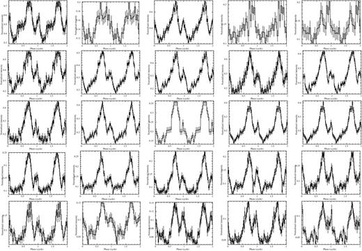
Pulse profiles of SGR 1745−2900 obtained from Chandra observations in the 0.3–10 keV energy range. Epoch increases from left to right, top to bottom. Two cycles are shown for clarity.
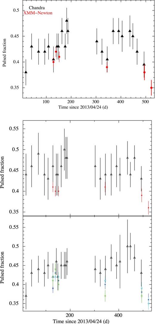
Temporal evolution of the pulsed fraction (see text for our definition). Uncertainties on the values were obtained by propagating the errors on the maximum and minimum count rates. Top panel: in the 0.3–10 keV band. Central panel: in the 0.3–3.5 band for the Chandra (black triangles) and XMM–Newton (red points) observations. Bottom panel: in the 3.5–10 band for the Chandra observations (black) and in the 3.5–5 (blue), 5–6.5 (light blue), and 6.5–10 keV (green) ranges for the XMM–Newton observations.
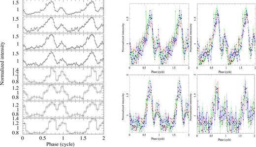
Pulse profiles of SGR 1745−2900 obtained from XMM–Newton/EPIC-pn observations. Two cycles are shown for clarity. Left: pulse profiles in the 0.3–10 keV energy band. Right: pulse profiles in the 0.3–3.5, 3.5–5, 5–6.5, and 6.5–10 keV energy bands (from left to right, top to bottom) for the first four observations. Black, red, green, and blue colours refer to the first, second, third, and fourth observation, respectively.
2.2 Spectral analysis of Chandra observations
For all the Chandra observations, we extracted the source counts from a 1.5-arcsec radius circular region centred on SGR 1745−2900. This corresponds to an encircled energy fraction of ∼85 per cent of the Chandra point spread function (PSF) at 4.5 keV. A larger radius would have included too many counts from the Sgr A* PSF, overestimating the flux of SGR 1745−2900 with only a marginal increase of the encircled energy fraction (less than ∼5 per cent). We extracted the background counts using three different regions: an annulus (inner and outer radius of 14 and 20 arcsec, respectively), four 2-arcsec radius circles arranged in a square centred on the source, or a 1.5-arcsec radius circle centred on the source position in an archival Chandra/ACIS-S observation (i.e. when the magnetar was still in quiescence). For grating observations we considered instead a circle of radius 10 arcsec as far as possible from the grating arms but including part of the diffuse emission present in the Galactic Centre.
For ‘non-grating’ observations, we created the source and background spectra, the associated redistribution matrix files, and ancillary response files using the specextract tool.3 For the three grating observations, we analysed only data obtained with the High Energy Grating (0.8–8 keV). In all cases SGR 1745−2900 was offset from the zeroth-order aim point, which was centred on the nominal Sgr A* coordinates [|$\rm RA = 17 ^h45^m 40{.\!\!^{{\mathrm{s}}}}00$|, Dec. = −29°00′28|${^{\prime\prime}_{.}}$|1 (J2000.0)]. We extracted zeroth-order spectra with the tgextract tool and generated redistribution matrices and ancillary response files using mkgrmf and fullgarf, respectively.
We grouped background-subtracted spectra to have at least 50 counts per energy bin, and fitted in the 0.3–8 keV energy band (0.8–8 keV for grating observations) with the xspec4 spectral fitting package (version 12.8.1g; Arnaud 1996), using the χ2 statistics. The photoelectric absorption was described through the tbabs model with photoionization cross-sections from Verner et al. (1996) and chemical abundances from Wilms, Allen & McCray (2000). The small Chandra PSF ensures a negligible impact of the background at low energies and allows us to better constrain the value of the hydrogen column density towards the source.
We estimated the impact of photon pile-up in the non-grating observations by fitting all the spectra individually. Given the pile-up fraction (up to ∼30 per cent for the first observation as determined with Webpimms, version 4.7), we decided to correct for this effect using the pile-up model of Davis (2001), as implemented in xspec. According to ‘The Chandra ABC Guide to Pile-up’,5 the only parameters allowed to vary were the grade-migration parameter (α), and the fraction of events in the source extraction region within the central, piled up, portion of the PSF. Including this component in the spectral modelling, the fits quality and the shape of the residuals improve substantially especially for the spectra of the first 12 observations (from obs ID 14702 to 15045), when the flux is larger. We then compared our results over the three different background extraction methods (see above) and found no significant differences in the parameters, implying that our reported results do not depend significantly on the exact location of the selected background region.
We fitted all non-grating spectra together, adopting four different models: a blackbody, a power law, the sum of two blackbodies, and a blackbody plus a power law. For all the models, we left all parameters free to vary. However, the hydrogen column density was found to be consistent with being constant within the errors6 among all observations and thus was tied to be the same. We then checked that the inclusion of the pile-up model in the joint fits did not alter the spectral parameters for the last 10 observations (from obs ID 16508 onwards), when the flux is lower, by fitting the corresponding spectra individually without the pile-up component. The values for the parameters are found to be consistent with being the same in all cases.
A fit with an absorbed blackbody model yields |$\chi ^2_\nu = 1.00$| for 2282 d.o.f., with a hydrogen column density |${N_{\rm H}} = 1.90(2) \times 10^{23}$| cm−2, temperature in the 0.76–0.90 keV range, and emitting radius in the 1.2–2.5 km interval. When an absorbed power-law model is used (|$\chi ^2_\nu =1.05$| for 2282 d.o.f.), the photon index is within the range 4.2–4.9, much larger than what is usually observed for this class of sources (see Mereghetti 2008; Rea & Esposito 2011 for reviews). Moreover, a larger absorption value is obtained (|${N_{\rm H}}\sim 3 \times 10^{23}$| cm−2). The large values for the photon index and the absorption are likely not intrinsic to the source, but rather an artefact of the fitting process which tends to increase the absorption to compensate for the large flux at low energies defined by the power law. The addition of a second component to the blackbody, i.e. another blackbody or a power law, is not statistically required (|$\chi ^2_\nu = 1.00$| for 2238 d.o.f. in both cases). We thus conclude that a single absorbed blackbody provides the best modelling of the source spectrum in the 0.3–8 keV energy range (see Table 3).
Taking the absorbed blackbody as a baseline, we tried to model all the spectra tying either the radius or the temperature to be the same for all spectra. We found |$\chi ^2_\nu = 1.38$| for 2303 d.o.f. when the radii are tied, with |${N_{\rm H}}= 1.94(2) \times 10^{23}$| cm−2, |$R_{\rm BB}=1.99_{-0.05}^{+0.06}$| km, and temperatures in the 0.66–0.97 keV range. We found instead |$\chi ^2_\nu = 1.04$| for 2303 d.o.f. when the temperatures are tied, with |${N_{\rm H}}= 1.89(2) \times 10^{23}$| cm−2, kTBB = 0.815(7) keV, and radii spanning from ∼1.1 to ∼3 km. The goodness of fit of the latter model improves considerably if the temperatures are left free to vary as well (F-test probability of ∼2 × 10⁻¹⁷; fitting the temperature evolution with a constant yields a poor |$\chi ^2_\nu =2.8$| for 24 d.o.f. in this case). We conclude that both the temperature and the size of the blackbody emitting region are varying. Zeroth-order spectral data of the three grating observations were fitted together and independently with this model, without including the pile-up component and fixing |${N_{\rm H}}$| to that obtained in non-grating fit: 1.9 × 1023 cm−2 (see Table 3 and Fig. 5).
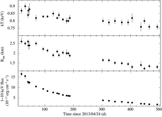
Temporal evolution of the spectral parameters for the blackbody model and of the 1–10 keV absorbed flux of SGR 1745−2900 from Chandra observations.
2.3 Spectral analysis of XMM–Newton observations
For all the XMM–Newton observations, we extracted the source counts from a circular region of radius 15 arcsec centred on the source PSF, and the background counts through the same circle at the same position in an archival (2011) XMM–Newton observation of the Galactic Centre (obs. ID 0694640301), when the magnetar was not detected and no transient events were identified within the source PSF. We built the light curves for the source and background event files to visually inspect and filter for high particle background flaring in the selected regions. We checked for the potential impact of pile-up using the epatplot task of sas: the observed pattern distributions for both single and double events are consistent with the expected ones (at a 1σ confidence level) for all the three cameras, proving that the XMM–Newton data are unaffected by pile-up.
We restricted our spectral analysis to photons having flag = 0 and pattern ≤4(12) for the pn (MOSs) data and created spectral redistribution matrices and ancillary response files. We co-added the spectral files of consecutive observations (obs. ID 0743630201-301 and 0743630401-501; see Table 1) to improve the fit statistics and reduce the background contamination. We then grouped the source spectral channels to have at least 200 counts per bin and fitted the spectra in the 2–12 keV range, given the high background contamination within the source PSF at lower energies. The spectral data extracted from the two MOS cameras gave values for the parameters and fluxes consistent with those obtained from the pn camera. To minimize the systematic errors introduced when using different instruments, we considered only the pn data, which provide the spectra with the highest statistics.
Because of the large PSF of XMM–Newton, it is not possible to completely remove the contamination of both the Galactic Centre soft X-ray diffuse emission and the emission lines from the supernova remnant Sgr A east, including in particular the iron line (Fe xxv; rest energy of 6.7 keV) and the sulfur line (S xv; rest energy of 2.46 keV) (see e.g. Maeda et al. 2002; Sakano et al. 2004; Ponti et al. 2010, Ponti et al. 2013; Heard & Warwick 2013). These features were clearly visible especially in the spectra of the last observations, when the flux is lower, and prevented us from obtaining a good spectral modelling in xspec. We thus decided to discard the energy interval comprising the Fe xxv line (6.4–7.1 keV) for all the spectra, as well as that associated with the S xv line (2.3–2.7 keV) for the spectrum of the last observations (obs. ID 0690441801, 0743630201-301, 0743630401-501), involving a loss of ∼9 per cent in the total number of spectral bins.
Based on the results of the Chandra spectral analysis, we fitted the data first with an absorbed blackbody model. The hydrogen column density was consistent with being constant at a 90 per cent confidence level among all observations and was tied to be the same in the spectral fitting. We obtained |$\chi ^2_\nu =2.2$| for 636 d.o.f., with large residuals at high energies. The latter disappear if an absorbed power-law component is added and the fit improves considerably (|$\chi ^2_\nu =1.13$| for 624 d.o.f.; see left-hand panel of Fig. 6). A fit with a two-blackbody model is statistical acceptable as well (|$\chi ^2_\nu =1.13$| for 624 d.o.f.) and yields temperatures of ∼2–4 keV and emitting radii of ∼0.04–0.12 km for the second blackbody. However, this model would be physically hard to justify, since it is unlikely that these large temperatures can be maintained on a neutron star surface for such a long time. As an alternative to these fits, we applied a 3D resonant cyclotron scattering model (NTZ; Nobili et al. 2008a,b; Zane et al. 2009), obtaining |$\chi ^2_\nu =1.14$| for 624 d.o.f. (see right-hand panel of Fig. 6). The hydrogen column densities and fluxes inferred both from the BB+PL and the NTZ models are consistent with each other within the errors (see Table 4). To test the robustness of our results, we compared the inferred parameters with those derived by fitting the spectra without filtering for the spectral channels and applying the varabs model for the absorption, which allows the chemical abundances of different elements to vary (only the sulfur and iron abundances were allowed to vary for the present purpose). We found consistent values over the two methods.
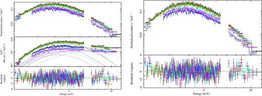
Results of the phase-averaged spectral analysis for the XMM–Newton/EPIC-pn observations of SGR 1745−2900. Left-hand panel: source spectra fitted together with an absorbed blackbody plus power-law model in the 2–12 keV range and after removal of the Fe xxv and S xv lines (see text). E2 f(E) unfolded spectra together with the contributions of the two additive components and residuals (in units of standard deviations) are also shown. Right-hand panel: source spectra fitted together with an absorbed 3D resonant cyclotron scattering model in the 2–12 keV range and after removal of the Fe xxv and S xv lines (see text). Residuals (in units of standard deviations) are also shown.
We conclude that both models successfully reproduce the soft X-ray part of the SGR 1745−2900 spectra up to ∼12 keV, implying that, similar to other magnetars, the reprocessing of the thermal emission by a dense, twisted magnetosphere produces a non-thermal component. The power law detected by XMM–Newton is consistent with that observed by NuSTAR (Kaspi et al. 2014), and its very low contribution below 8 keV is consistent with its non-detection in our Chandra data.
2.4 Pulse phase-resolved spectral (PPS) analysis
To search for spectral variability as a function of rotational phase and time, we first extracted all the spectra of the Chandra observations selecting three pulse phase intervals (see Fig. 2): peak (ϕ = 0.5–0.9), minimum (ϕ = 0.2–0.5), and secondary peak (ϕ = 0.9–1.2). We adopted the same extraction regions and performed the same data analysis as for the phase-averaged spectroscopy.
For each of the three different phase intervals, we fitted the spectra of all Chandra observations jointly in the 0.3–8 keV energy band with an absorbed blackbody model and tying the hydrogen column density to be the same in all the observations (the pile-up model was included). Since the values of the column density are consistent with being the same at a 90 per cent confidence level (1.90(4) × 1023, 1.82(4) × 1023, and |$1.83_{-0.04}^{+0.05} \times 10^{23}$| cm−2 for the peak, the secondary peak, and the minimum, respectively), we fixed |${N_{\rm H}}$| to 1.9 × 1023 cm−2, i.e. to the best-fitting value determined with the phase-averaged spectroscopy (see Table 3). We obtained a good fit in all cases, with |$\chi ^2_\nu =1.04$| for 1005 d.o.f. for the peak, |$\chi ^2_\nu =1.10$| for 635 d.o.f. for the secondary peak, and |$\chi ^2_\nu = 0.99$| for 713 d.o.f. for the pulse minimum. The fit residuals were not optimal for energies ≳ 6–7 keV for the peak spectra, due to the larger pile-up fraction. We extracted the source counts excluding the central piled up photons (within a radial distance of 0.7 arcsec from the source position), and repeated the analysis for the peak spectra: the residuals are now well shaped, and the inferred values for the spectral parameters did not change significantly.
The temporal evolution of the blackbody temperature and radius for both the peak and the pulse minimum are shown in Fig. 7. No particular trend is observed for the inferred temperatures, whereas the size of the emitting region is systematically lower for the pulse minimum. This is consistent with a viewing geometry that allows us to observe the hotspot responsible for the thermal emission almost entirely at the peak of the pulse profile, and only for a small fraction at the minimum of the pulsation.
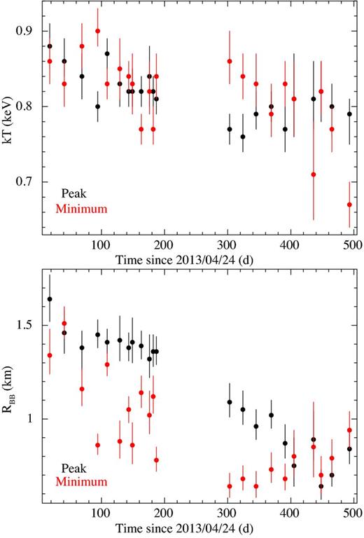
Evolution of the blackbody temperatures (left-hand panel) and radii (right-hand panel) for the peak (black points) and the minimum (red points) of the pulse profile for the Chandra observations.
The higher statistics of the XMM–Newton/EPIC-pn data allowed us to put more stringent constraints on the variations of the X-ray spectral parameters along the spin phase. We extracted the background-subtracted spectra in six different phase intervals for each observation, as shown in Fig. 8. We fitted all spectra with a BB+PL model, adopting the same prescriptions used for the phase-averaged spectroscopy in the filtering of the spectral channels. We tied the hydrogen column density and the power-law photon indices to the best-fitting values determined with the phase-averaged analysis (see Table 4). We obtained statistically acceptable results in all cases. The evolutions of the blackbody temperature and emitting radius as a function of the rotational phase for all the observations are shown in Fig. 8. Variability of both the parameters along the rotational phase is more significant during the first observation (a fit with a constant yields |$\chi ^2_\nu =2.6$| for 5 d.o.f. in both cases) than in the following observations (|$\chi ^2_\nu \le 1.4$| for 5 d.o.f. in all cases).
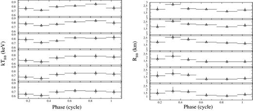
Evolution of the blackbody temperatures (left) and radii (right) as a function of the rotational phase for the XMM–Newton observations. Spectra of consecutive observations were co-added (obs. ID 0743630201-301 and 0743630401-501; see the two lower panels).
To search for possible phase-dependent absorption features in the X-ray spectra of SGR 1745−2900 (similarly to the one detected in SGR 0418+5729; Tiengo et al. 2013), we produced images of energy versus phase for each of the eight EPIC-pn observations. We investigated different energy and phase binnings. In Fig. 9 we show the image for the observation with the highest number of counts (obs. ID 0724210201), produced by binning the source counts into 100 phase bins and 100 eV wide energy channels. The spin period modulation is clearly visible, as well as the large photoelectric absorption below 2 keV. For all observations we then divided these values first by the average number of counts in the same energy bin and then by the corresponding 0.3–10 keV count rate in the same phase interval. No prominent features can be seen in any of the images.
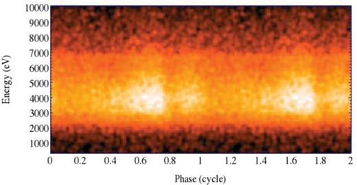
Energy versus phase image for the XMM–Newton observation with the highest number of counts (obs. ID 0724210201). The image was obtained by binning the EPIC-pn source counts into 100 phase bins and energy channels of 100 eV, to better visualize the shape of the pulse profile and its dependence on energy.
2.5 X-ray brightness radial profiles
For all the Chandra observations, we used the Chandra Ray Tracer (chart;7 Carter et al. 2003) to simulate the best available PSF for SGR 1745−2900, setting the exposure time of each simulation equal to the exposure time of the corresponding observation. For the input spectrum in chart we employed the blackbody spectrum of Table 3, accounting for the pile-up. We then projected the PSF rays on to the detector plane via the Model of AXAF Response to X-rays software (marx,8 version 4.5.0; Wise et al. 2003). We extracted the counts of both the simulated PSFs and the ACIS event files through 50 concentric annular regions centred on the source position and extending from 1 to 30 pixels (1 ACIS-S pixel corresponds to 0.492 arcsec). We then generated the X-ray brightness radial profiles and normalized the nominal one (plus a constant background) to match the observed one at a radial distance of 4 pixels, i.e. at a distance at which pile-up effects are negligible. A plot of the observed and simulated surface brightness fluxes (in units of counts × pixel−2) versus radial distance from the position of SGR 1745−2900 is shown in Fig. 10 for the observation with the highest number of counts (obs. ID 15041).
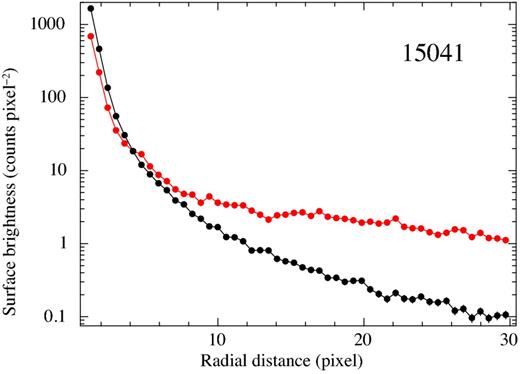
Radial profile of the surface brightness for both the ACIS-S image of SGR 1745−2900 (red dots) and the chart/marx PSF plus a constant background (black dots) for the observation with the highest number of counts (obs. ID 15041). The simulated surface brightness has been normalized to match the observed one at 4 pixels (one ACIS-S pixel corresponds to 0.492 arcsec). Extended emission around SGR 1745−2900 is clearly detected in all the observations.
Chandra spectral fitting results obtained with an absorbed blackbody model (|$\chi ^2_\nu = 1.00$| for 2282 d.o.f.). The hydrogen column density was tied to be the same in all the observations, resulting in |${N_{\rm H}}= 1.90(2) \times 10^{23}$| cm−2 (photoionization cross-sections from Verner et al. 1996 and chemical abundances from Wilms et al. 2000). The α is a parameter of the xspec pile-up model (see Davis 2001 and ‘The Chandra ABC Guide to Pile-up’). The pile-up model was not included when fitting the HETG/ACIS-S spectra (obs. ID 15040, 15651, 15654). The blackbody radius and luminosity are calculated assuming a source distance of 8.3 kpc (see e.g. Genzel et al. 2010). Fluxes and luminosities were calculated after removing the pile-up model. All errors are quoted at a 90 per cent confidence level for a single parameter of interest (Δχ2 = 2.706).
| Obs. ID | α | kTBB | RBB | 1–10 keV absorbed flux | 1–10 keV luminosity |
|---|---|---|---|---|---|
| (keV) | (km) | (10−12 erg cm−2 s−1) | (1035 erg s−1) | ||
| 14702 | 0.47(6) | 0.87(2) | 2.6|$_{-0.1}^{+0.2}$| | 16.5|$_{-0.8}^{+1.0}$| | 4.7(3) |
| 15040 | – | 0.90(2) | 2.5(1) | 15.5|$_{-1.3}^{+0.03}$| | 4.7(4) |
| 14703 | 0.47|$_{-0.06}^{+0.07}$| | 0.84(2) | 2.6(1) | 12.7|$_{-0.6}^{+0.5}$| | 3.9(3) |
| 15651 | – | 0.87(3) | 2.4(2) | 12.5|$_{-0.9}^{+0.07}$| | 3.8(4) |
| 15654 | – | 0.88(4) | 2.4(2) | 12.4|$_{-0.9}^{+0.05}$| | 3.5(4) |
| 14946 | 0.43(8) | 0.82(2) | 2.5(1) | 10.5|$_{-0.7}^{+0.4}$| | 3.3(3) |
| 15041 | 0.42|$_{-0.05}^{+0.06}$| | 0.83(1) | 2.22|$_{-0.09}^{+0.10}$| | 9.3|$_{-0.3}^{+0.2}$| | 2.9 |$_{-0.4}^{+0.2}$| |
| 15042 | 0.55(7) | 0.83(1) | 2.14(9) | 8.3(3) | 2.6|$_{-0.4}^{+0.2}$| |
| 14945 | 0.4(1) | 0.85(2) | 1.9(1) | 7.6|$_{-0.4}^{+0.3}$| | 2.3(2) |
| 15043 | 0.51(8) | 0.82(1) | 2.09|$_{-0.09}^{+0.10}$| | 7.2|$_{-0.3}^{+0.2}$| | 2.4 |$_{-0.3}^{+0.2}$| |
| 14944 | 0.6(1) | 0.84(2) | 1.9(1) | 7.0(4) | 2.2|$_{-0.3}^{+0.2}$| |
| 15044 | 0.48|$_{-0.08}^{+0.09}$| | 0.81(1) | 2.03|$_{-0.09}^{+0.10}$| | 6.4(2) | 2.1|$_{-0.3}^{+0.2}$| |
| 14943 | 0.4(1) | 0.80(2) | 2.0|$_{-0.1}^{+0.2}$| | 6.1|$_{-0.4}^{+0.2}$| | 2.0(3) |
| 14704 | 0.5(1) | 0.80|$_{-0.01}^{+0.02}$| | 2.0(1) | 6.0|$_{-0.3}^{+0.2}$| | 2.0(2) |
| 15045 | 0.42(9) | 0.82|$_{-0.01}^{+0.02}$| | 1.88(9) | 5.9|$_{-0.2}^{+0.1}$| | 1.9 |$_{-0.2}^{+0.1}$| |
| 16508 | 0.6(2) | 0.80|$_{-0.01}^{+0.02}$| | 1.65|$_{-0.10}^{+0.09}$| | 3.8|$_{-0.2}^{+0.1}$| | 1.3 |$_{-0.2}^{+0.1}$| |
| 16211 | 0.3(2) | 0.79(2) | 1.64|$_{-0.09}^{+0.10}$| | 3.6|$_{-0.2}^{+0.1}$| | 1.2(2) |
| 16212 | 0.4(2) | 0.80(2) | 1.51|$_{-0.09}^{+0.10}$| | 3.2(1) | 1.1(1) |
| 16213 | 0.3(2) | 0.79(2) | 1.49|$_{-0.07}^{+0.08}$| | 3.1(1) | 1.1(1) |
| 16214 | 0.4(2) | 0.79(2) | 1.45|$_{-0.09}^{+0.10}$| | 2.8(1) | 1.0(1) |
| 16210 | 0.4(2) | 0.82(3) | 1.3(1) | 2.70(7) | 0.9(1) |
| 16597 | 0.5(2) | 0.76(3) | 1.4|$_{-0.1}^{+0.2}$| | 2.20|$_{-0.05}^{+0.04}$| | 0.8(1) |
| 16215 | 0.4(2) | 0.80(2) | 1.22|$_{-0.08}^{+0.09}$| | 2.11(4) | 0.7(1) |
| 16216 | 0.3(2) | 0.76(2) | 1.34|$_{-0.09}^{+0.10}$| | 1.91(4) | 0.7(1) |
| 16217 | 0.3(2) | 0.76(2) | 1.3(1) | 1.80(3) | 0.67(9) |
XMM–Newton/EPIC-pn spectral fitting results obtained with an absorbed blackbody plus power-law model (|$\chi ^2_\nu =1.13$| for 624 d.o.f.) and an absorbed 3D resonant cyclotron scattering model (|$\chi ^2_\nu =1.14$| for 624 d.o.f.). βbulk denotes the bulk motion velocity of the charges in the magnetosphere and Δϕ is the twist angle. For both models the hydrogen column density was tied to be the same in all the observations, yielding |${N_{\rm H}}=1.86_{-0.08}^{+0.10} \times 10^{23}$| cm−2 for the former and |${N_{\rm H}}=1.86_{-0.03}^{+0.05} \times 10^{23}$| cm−2 for the latter (photoionization cross-sections from Verner et al. 1996, and chemical abundances from Wilms et al. 2000). The blackbody emitting radius and luminosity are calculated assuming a source distance of 8.3 kpc (see e.g. Genzel et al. 2010). Fluxes were determined with the cflux model in xspec. All errors are quoted at a 90 per cent confidence level for a single parameter of interest (Δχ2 = 2.706).
| Obs. ID | kTBB | RBB | Γ | PL norm | 1–10 keV BB/PL abs flux | 1–10 keV BB/PL luminosity |
|---|---|---|---|---|---|---|
| (keV) | (km) | (10−3) | (10−12 erg cm−2 s−1) | (1035 erg s−1) | ||
| BB+PL | ||||||
| 0724210201 | 0.79(3) | 1.9(2) | 2.3|$_{-0.7}^{+0.5}$| | 4.5|$_{-3.5}^{+8.9}$| | 5.0(1)/3.3(2) | 1.7|$_{-0.3}^{+0.2}$|/1.0|$_{-0.3}^{+0.4}$| |
| 0700980101 | 0.78(3) | 2.1(2) | 1.7|$_{-1.3}^{+0.8}$| | <6.8 | 5.7(1)/2.2(2) | 2.0(3)/0.5(3) |
| 0724210501 | 0.79(4) | 2.1|$_{-0.2}^{+0.3}$| | 2.3|$_{-0.6}^{+0.5}$| | <4.5 | 5.8(1)/1.8(2) | 2.0|$_{-0.2}^{+0.1}$|/0.3|$_{-0.2}^{+0.3}$| |
| 0690441801 | 0.72|$_{-0.04}^{+0.03}$| | 1.6(3) | 2.6|$_{-0.8}^{+0.5}$| | 4.5|$_{-3.8}^{+8.8}$| | 1.9(1)/2.1|$_{-0.2}^{+0.1}$| | 0.8(2)/0.8(3) |
| 0743630201-301 | 0.71(6) | 1.3(3) | 2.1|$_{-1.4}^{+0.7}$| | 1.6|$_{-1.5}^{+6.1}$| | 1.2(1)/1.7(2) | 0.5(2)/0.4(3) |
| 0743630401-501 | 0.67|$_{-0.07}^{+0.10}$| | 1.2(5) | 2.0|$_{-0.7}^{+0.4}$| | 6.3|$_{-4.9}^{+9.7}$| | 0.7(1)/2.0(4) | 0.3(2)/<0.5 |
| Obs. ID | kT | βbulk | Δϕ | NTZ norm | 1–10 keV abs flux | 1–10 keV luminosity |
| (keV) | (rad) | (10−1) | (10−12 erg cm−2 s−1) | (1035 erg s−1) | ||
| NTZ | ||||||
| 0724210201 | 0.85(2) | 0.72|$_{-0.40}^{+0.09}$| | 0.40|$_{-0.24}^{+0.04}$| | 1.62|$_{-0.12}^{+0.07}$| | 8.3(1) | 2.5(2) |
| 0700980101 | 0.85|$_{-0.03}^{+0.02}$| | 0.70|$_{-0.34}^{+0.04}$| | 0.40|$_{-0.23}^{+0.03}$| | 1.58|$_{-0.11}^{+0.14}$| | 7.9(1) | 2.3(2) |
| 0724210501 | 0.84(2) | 0.6(2) | 0.41|$_{-0.25}^{+0.02}$| | 1.5(1) | 7.6(1) | 2.3(3) |
| 0690441801 | 0.77|$_{-0.06}^{+0.04}$| | 0.5|$_{-0.2}^{+0.3}$| | 0.42|$_{-0.25}^{+0.06}$| | 0.94|$_{-0.07}^{+0.10}$| | 4.0(1) | 1.3(2) |
| 0743630201-301 | 0.76|$_{-0.10}^{+0.07}$| | >0.2 | 0.43|$_{-0.03}^{+0.64}$| | 0.61|$_{-0.06}^{+0.09}$| | 2.9(1) | 0.9(3) |
| 0743630401-501 | 0.65|$_{-0.24}^{+0.07}$| | 0.32|$_{-0.09}^{+0.11}$| | 0.60|$_{-0.17}^{+0.78}$| | 0.68|$_{-0.07}^{+0.27}$| | 2.7(1) | 0.9(3) |
Extended emission around SGR 1745−2900 is clearly detected in all the observations, and it is likely dominated by the intense Galactic Centre diffuse emission. A detailed analysis of the diffuse emission, including its spatial extension and spectral properties, is beyond the scope of this paper, and will be published in a subsequent work.
3 DISCUSSION
3.1 Outburst evolution and comparison with other magnetars
The past decade has seen a great success in detecting magnetar outbursts, mainly thanks to the prompt response and monitoring of the Swift mission, and to the dedicated follow-up programs of Chandra, XMM–Newton, and more recently, NuSTAR. The detailed study of about 10 outbursts has shown many common characteristics (see Rea & Esposito 2011, for a review; see also Fig. 11), although the precise triggering mechanism of these outbursts, as well as the energy reservoir responsible for sustaining the emission over many months, remains uncertain.
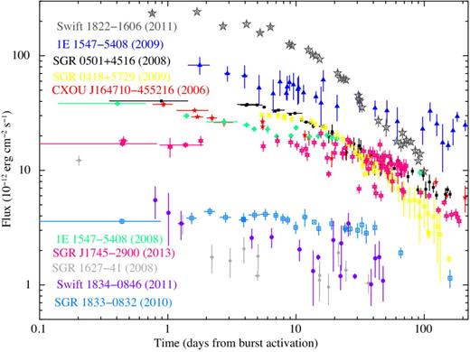
Flux decay of all magnetar outbursts monitored with imaging instruments. Fluxes are absorbed in the 1–10 keV energy range (adapted and updated from Rea & Esposito 2011).
All the outbursts that have been monitored with sufficient detail are compatible with a rapid (<d) increase in luminosity up to a maximum of a few 1035 erg s−1 and a thermally dominated X-ray spectrum which softens during the decay. In the case of SGR 0501+4516 and 1E 1547−5408, a non-thermal component extending up to 100–200 keV appears at the beginning of the outburst, and becomes undetectable after weeks/months (Rea et al. 2009; Bernardini et al. 2011; Kuiper et al. 2012).
The initial behaviour of the 2013 outburst decay of SGR 1745−2900 was compatible with those observed in other magnetars. The outburst peak, the thermal emission peaked at about 1 keV, the small radiating surface (about 2 km in radius), and the overall evolution in the first few months were consistent with the behaviour observed in other outbursts. However, after an additional year of X-ray monitoring, it became clear that the subsequent evolution of SGR 1745−2900 showed distinct characteristics. The source flux decay appears extremely slow: it is the first time that we observe a magnetar with a quiescent luminosity <1034 erg s−1 remaining at a luminosity >1035 erg s−1 for more than 1 yr, and with a temperature decreasing by less than 10 per cent from the initial ∼1 keV. A further interesting feature of this source is that the non-thermal component (as detected by XMM–Newton) persisted on a very long temporal baseline during the outburst evolution. The flux due to the power-law component does not change significantly in time and, as a result, its fractional contribution to the total flux is larger at late times: ∼520 d after the outburst onset, ≲ 50 per cent of the 1–10 keV absorbed flux is due to the non-thermal component.
We first modelled the decay empirically to gauge the characteristic decay time-scales. We adopted three different functions to model the blackbody temperature, radius, and 1–10 keV absorbed flux temporal evolutions (see Fig. 5): (i) a linear model; (ii) a power law: f (t) = f0, PL t−Γ; (iii) an exponential: f (t) = f0, exp exp[ − (t − t0)/τ], where t0 is the epoch of the first burst detected (which we fixed to 2013 April 24 in all cases) and τ is the e-folding time.
The temporal evolution of the magnetar temperature is well represented by a linear model (|$\chi ^2_\nu =0.7$| for 23 d.o.f.), with initial temperature kTBB, 0 = 0.85(1) keV and slope (−1.77 ± 0.04) × 10−4. The hotspot shrinking is best modelled by an exponential (|$\chi ^2_\nu =0.8$| for 23 d.o.f.). Best-fitting parameters are τ = 640 ± 62 d and initial radius RBB, 0 = 2.60 ± 0.08 km. The shape of the flux decline appears to change in time and in fact none of these models can accurately describe the magnetar flux overall decay. The flux decay during the first 100 d since the outburst onset is well modelled by a linear plus exponential model with τ = 37 ± 2 d (|$\chi ^2_\nu$| = 1.5 for 4 d.o.f.). After ∼100 d, the best-fitting model turns out to be an exponential with τ = 253 ± 5 d (|$\chi ^2_\nu$| = 1.4 for 15 d.o.f.).
3.2 Crustal cooling modelling
We applied the crustal cooling model (see e.g. Pons & Rea 2012) to the data collected during the 1.5-yr outburst of SGR 1745−2900. Although this model was successful in explaining several other magnetar outbursts (Rea et al. 2012, 2013a), in this case we could not reproduce the very slow cooling and high luminosity observed for this source. We ran several models varying the total injected energy, the angular size, and the depth of the region where the energy is released, but we could not find any set of parameters that fit the data.
In the framework of the starquake model, the maximum temperature reached in the region where the energy is released is limited by neutrino emission processes. This internal temperature determines the maximum surface temperature and therefore the luminosity at which the outburst peaks during the first few days. For injected energies >1043 erg, there is no significant increase in the peak luminosity because the crustal temperature saturates (at about 3–5 × 10⁹ K) due to the efficient neutrino processes. After reaching the maximum luminosity (between 1 h and 1 d depending on the depth and injection rate), the cooling curve tracks the thermal relaxation of the crust. Independent of the initial injected energy and surface temperature, the luminosity is expected to drop below 1035 erg s−1 after <20–30 d (see e.g. fig. 1 in Pons & Rea 2012), due to neutrino emission processes in the crust (mainly plasmon decay, and probably neutrino synchrotron for magnetar field strengths).
In Fig. 12 (left-hand panel, lower curves) we show an example of the expected cooling curve of a magnetar with the same characteristics of SGR 1745−2900. We assume that a sudden large energy release, E ≃ 1045 erg, heats up a layer of the outer crust up to 3 × 10⁹ K. We also assume that the event affects the entire magnetar surface, to create the most favourable scenario (the luminosity simply scales with the area of the emitting region), and that the layer where the energy is injected extends from an external boundary at ρOUT ∼ 3 × 10⁹ g cm−3, to an inner boundary at ρIN ∼ 2 and 4 × 10¹⁰ g cm−3 (we show these two cases in the two lower curves of Fig. 12, left-hand panel). It is clear that, even in this most favourable case, the high luminosities observed at late times are difficult to reconcile with any cooling model. In particular, injecting more energy or changing ρOUT will only affect the peak luminosity during the first days or weeks. On the other hand, injecting energy deeper into the crust (i.e. at higher ρIN) is expected to change the late-time evolution only slightly. This can be seen by comparing the solid and dashed lines in the left-hand panel of Fig. 12, which correspond to ρIN = 2 and 4 × 10¹⁰ g cm−3, respectively.
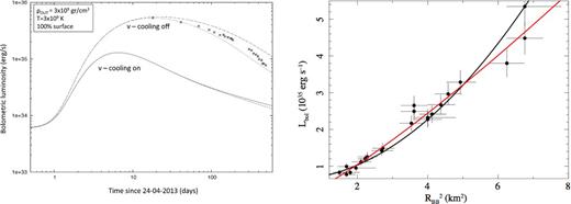
Left-hand panel: crustal cooling curves attempting at modelling the luminosity decrease of SGR 1745−2900. Luminosities are bolometric and calculated assuming a distance of 8.3 kpc. For the neutrino cooling on and off set of curves, the lower and upper curves are relative to ρIN = 2 and 4 × 10¹⁰ g cm−3, respectively. Right-hand panel: bolometric luminosity as a function of the square of the blackbody radius at infinity. Solid lines represent the fits with a quadratic function (black) and a generic power law (α = 1.23(8); red).
For illustrative purposes, we also show the cooling curves obtained when plasmon and synchrotron neutrino processes are switched off (see the upper curves in the left-hand panel of Fig. 12). These provide a much closer match to the data; however, there is no clear reason why these neutrino processes should not operate in these conditions. This example is only meant to highlight the relevance of understanding neutrino processes in the crust, especially under the presence of strong fields. Another possibility to fit the data is to tune the energy injection, which must be maintained during the first ∼200 d, resulting in a higher luminosity at late times. If we assume that only a region 5 km in radius is affected (this is closer to the ∼2 km emitting region observed), we need a continuous injection of at least ∼1044 erg s−1 (d−1) for about 200 d, which results in a total energy of a few 1046 erg. While this energy budget may not be unrealistic, a physical mechanism that can operate for such a long time-scale is not known. A possibility might be a continuous injection of energy to keep the surface at high temperatures for so long, although in this latter case we should possibly expect more SGR-like bursts during the first hundreds days.
3.3 Bombardment by magnetospheric currents in a bundle
In this section we discuss the possibility that the prolonged high luminosity of SGR 1745−2900 is in part due to external particle bombardment as a consequence of the existence of a twisted magnetic field bundle. A valid alternative model to the crustal cooling scenario invokes the presence of magnetospheric currents flowing along a gradually shrinking magnetic bundle, and heating the surface from outside. According to Beloborodov (2007, 2013), this bundle can untwist on different time-scales: (i) in the equatorial regions of the magnetosphere, where the magnetic field reaches a few stellar radii, currents are dissipated after weeks or months, while (ii) at higher latitudes (close to the poles), a bundle may untwist more slowly, possibly in 1–10 yr. Here, particles can reach Lorentz factors of a few tens (Beloborodov 2007). In this scenario, a quasi-steady-state outflow of electrons and positrons is maintained thanks to magnetic pair production close to the surface. The non-negligible electric voltage along the magnetic field lines and the radiative force due to Compton scattering regulates the streams of positrons and electrons along the field line.
The presence of a non-thermal component observed by NuSTAR (Mori et al. 2013; Kaspi et al. 2014), and confirmed also by our XMM–Newton observations on a much longer temporal baseline, is suggestive of a large density of magnetospheric particles which boost thermal photons emitted from the surface via resonant Compton scattering, providing the power-law component. In this context, the observed ∼2 km size of the emitting blackbody is consistent with a relatively small j-bundle. In the scenario in which the outburst evolution is dominated by an untwisting bundle and the poloidal magnetic field has a dipole geometry, the luminosity is expected to decrease with the square of the blackbody area (|$A_{\rm b}= 4 \pi R_{{\rm BB}}^2$|; Beloborodov 2007, 2009). A flatter dependence may arise from a more complex field geometry. In Fig. 12 we show the fits of the bolometric luminosity as a function of |$R_{{\rm BB}}^2$| with two different models, a quadratic function |$L_{\rm bol} \propto A_{\rm b}^2$| (black line; |$\chi _{\rm \nu }^2 = 1.3$| for 23 d.o.f.) and a power law |$L_{\rm bol} \propto A_{\rm b}^{\alpha }$| (red line; |$\chi _{\rm \nu }^2 = 0.8$| for 23 d.o.f.). For the latter model we find α = 1.23(8). Interestingly, a similar relation was observed also for the outburst decay of SGR 0418+5729 (Rea et al. 2013a) and CXOU J1647−4552 (An et al. 2013).
According to Beloborodov (2013), both the Lorentz factor and the pair multiplicity change along the magnetic field lines, with typical values of |${\cal M}\sim 100$| (i.e. efficient pair creation), Γ ∼ 10 in the largest magnetic field loops, and |${\cal M} \sim 1$| (i.e. charge-separated plasma), Γ ∼ 1 in the inner part of the magnetosphere. The previous equality cannot be satisfied for a typical temperature of ∼0.8–1 keV, unless the magnetic field changes over an exceedingly small length-scale, a few metres at most. It appears, therefore, very unlikely that a single flow can explain both surface heating and resonant up-scattering.
4 CONCLUSIONS
The spectacular angular resolution of Chandra and the large effective area of XMM–Newton, together with an intense monitoring of the Galactic Centre region, has allowed us to collect an unprecedented data set covering the outburst of SGR 1745−2900, with very little background contamination (which can be very severe in this region of the Milky Way).
The analysis of the evolution of the spin period allowed us to find three different timing solutions between 2013 April 29 and 2014 August 30, which show that the source period derivative has changed at least twice, from 6.6 × 10⁻¹² s s−1 in 2013 April at the outburst onset, to 3.3 × 10⁻¹¹ s s−1 in 2014 August. While the first |$\dot{P}$| change could be related with the occurrence of an SGR-like burst (Kaspi et al. 2014), no burst has been detected from the source close in time to the second |$\dot{P}$| variation (although we cannot exclude it was missed by current instruments). This further change in the rotational evolution of the source might be related with the timing anomaly observed in the radio band around the end of 2013 (Lynch et al. 2015), unfortunately during our observing gap.
The 0.3–8 keV source spectrum is perfectly modelled by a single blackbody with temperature cooling from ∼0.9 to 0.75 keV in about 1.5 yr. A faint non-thermal component is observed with XMM–Newton. It dominates the flux at energies >8 keV at all the stages of the outburst decay, with a power-law photon index ranging from ∼1.7 to ∼2.6. It is most probably due to resonant Compton scattering on to non-relativistic electrons in the magnetosphere.
Modelling the outburst evolution with crustal cooling models has difficulty in explaining the high luminosity of this outburst and its extremely slow flux decay. If the outburst evolution is indeed due to crustal cooling, then magnetic energy injection needs to be continuous over at least the first ∼200 d.
The presence of a small twisted bundle sustaining currents bombarding the surface region at the base of the bundle, and keeping the outburst luminosity so high, appears a viable scenario to explain this particular outburst. However, detailed numerical simulations are needed to confirm this possibility.
This source is rather unique, given its proximity to Sgr A*. In particular, it has a >90 per cent probability of being in a bound orbit around Sgr A* according to our previous N-body simulations (Rea et al. 2013b), and the recent estimates inferred from its proper motion (Bower et al. 2015). We will continue monitoring the source with Chandra and XMM–Newton for the coming year.
FCZ and NR are supported by an NWO Vidi Grant (PI: Rea) and by the European COST Action MP1304 (NewCOMPSTAR). NR, AP, DV, and DFT acknowledge support by grants AYA2012-39303 and SGR2014-1073. AP is supported by a Juan de la Cierva fellowship. JAP acknowledges support by grant AYA 2013-42184-P. PE acknowledges a Fulbright Research Scholar grant administered by the US–Italy Fulbright Commission and is grateful to the Harvard–Smithsonian Center for Astrophysics for hosting him during his Fulbright exchange. DH acknowledges support from Chandra X-ray Observatory (CXO) Award Number GO3-14121X, operated by the Smithsonian Astrophysical Observatory for and on behalf of NASA under contract NAS8-03060, and also by NASA Swift grant NNX14AC30G. GP acknowledges support via an EU Marie Curie Intra-European fellowship under contract no. FP-PEOPLE-2012-IEF- 331095 and the Bundesministerium für Wirtschaft und Technologie/Deutsches Zentrum für Luft-und Raumfahrt (BMWI/DLR, FKZ 50 OR 1408) and the Max Planck Society. RP acknowledges partial support by Chandra grants (awarded by SAO) G03-13068A and G04-15068X. RPM acknowledges funding from the European Commission Seventh Framework Programme (FP7/2007-2013) under grant agreement no. 267251. FCZ acknowledges CSIC-IEEC for very kind hospitality during part of the work and Geoffrey Bower for helpful discussions. The scientific results reported in this paper are based on observations obtained with the Chandra X-ray Observatory and XMM–Newton, an ESA science mission with instruments and contributions directly funded by ESA Member States and NASA. This research has made use of software provided by the ChandraX-ray Center (CXC) in the application package ciao, and of softwares and tools provided by the High Energy Astrophysics Science Archive Research Center (HEASARC), which is a service of the Astrophysics Science Division at NASA/GSFC and the High Energy Astrophysics Division of the Smithsonian Astrophysical Observatory.
Ancillary response files are automatically corrected to account for continuous degradation in the ACIS CCD quantum efficiency.
Here, and in the following, uncertainties are quoted at the 90 per cent confidence level, unless otherwise noted.
