Combining radiative transfer and diffuse interstellar medium physics to model star formation

Bate, Matthew R.; Keto, Eric R.

doi:10.1093/mnras/stv451

Abstract

We present a method for modelling star-forming clouds that combines two different models of the thermal evolution of the interstellar medium (ISM). In the combined model, where the densities are low enough that at least some part of the spectrum is optically thin, a model of the thermodynamics of the diffuse ISM is more significant in setting the temperatures. Where the densities are high enough to be optically thick across the spectrum, a model of flux-limited diffusion is more appropriate. Previous methods either model the low-density ISM and ignore the thermal behaviour at high densities (e.g. inside collapsing molecular cloud cores), or model the thermal behaviour near protostars but assume a fixed background temperature (e.g. ≈10 K) on large scales. Our new method treats both regimes. It also captures the different thermal evolution of the gas, dust, and radiation separately. We compare our results with those from the literature, and investigate the dependence of the thermal behaviour of the gas on the various model parameters. This new method should allow us to model the ISM across a wide range of densities and, thus, develop a more complete and consistent understanding of the role of thermodynamics in the star formation process.

astrochemistry, hydrodynamics, radiative transfer, methods: numerical, stars: formation, ISM: general

1 INTRODUCTION

The thermal behaviour of interstellar gas is of fundamental importance for star formation. To initiate star formation, the thermal pressure must be insufficient to support the gas against gravitational collapse (Jeans 1929). Further evolution also depends on the thermodynamics and density structure, with a variety of different outcomes being possible such as the formation of a single polytrope or fragmentation into many clouds (Hoyle 1953; Hunter 1962; Layzer 1963; Tohline 1980; Rozyczka 1983). Larson (1985, 2005) emphasized the importance of the relationship between temperature and density in the interstellar medium (ISM), and Whitworth, Boffin & Francis (1998) emphasized the importance of the transition from molecular cooling to dust cooling. The typical decrease in gas temperature from T_g ∼ 1000 K at number densities of hydrogen nuclei of n_H ∼ 1 cm⁻³ to T_g ∼ 10 K at densities of n_H ∼ 10⁴ cm⁻³ promotes fragmentation, while the transition to an isothermal regime or temperature that increases with density above n_H ∼ 10⁴ cm⁻³ may help to produce a characteristic stellar mass (Larson 1985, 2005; Jappsen et al. 2005; Bonnell, Clarke & Bate 2006; Elmegreen, Klessen & Wilson 2008). Chemical reactions that control the abundances of gas phase coolants, and therefore radiative equilibrium, may affect this transition and the formation of molecular cloud cores. At even higher densities, deep within collapsing molecular cloud cores, different phases of collapse are believed to occur as the gas becomes optically thick and later as molecular hydrogen dissociates (Larson 1969). The treatment of radiative transfer can be crucial for determining whether the core fragments into multiple protostars or not (Boss et al. 2000; Krumholz 2006; Whitehouse & Bate 2006).

Previous radiation hydrodynamical simulations of star cluster formation demonstrate the importance of radiative feedback from protostars to correctly capture fragmentation and produce realistic numbers of brown dwarfs (Bate 2009; Offner et al. 2009). Whereas barotropic calculations of star cluster formation produce characteristic stellar masses that depend on the initial Jeans mass in the cloud (Bate & Bonnell 2005), Bate (2009) showed that radiative feedback reduces this dependence on the initial conditions. This may help to explain the apparent universality of the stellar initial mass function (IMF), at least in recent epochs (see also Krumholz 2011). Indeed, some recent radiation hydrodynamical simulations of star cluster formation have been quite successful in reproducing the observed IMF and other properties of stellar systems (Bate 2012, 2014; Krumholz, Klein & McKee 2012).

However, to date, radiation hydrodynamical simulations of star formation have been restricted to modelling dense molecular clouds and assuming that the only significant sources of radiation are the protostars themselves. In this case, the gas temperature at large distances from the protostars is assumed to be ≈10 K. However, this approximation is generally invalid at densities n_H ≲ 10⁴ cm⁻³ with solar metallicities, and is invalid at even higher densities at lower metallicities, if at all.

Informed by the vast literature on the physics, thermodynamics, and chemistry of the diffuse ISM (see the thorough review provided by Tielens 2005) and collapsing clouds with different metallicities (e.g. Omukai 2000; Omukai et al. 2005), interest has grown in studying the formation and evolution of molecular clouds using three-dimensional hydrodynamical calculations coupled with chemistry. Initial calculations treated only the formation of molecular hydrogen (Dobbs, Bonnell & Pringle 2006; Dobbs & Bonnell 2007; Glover & Mac Low 2007a,b; Micic et al. 2012). More recent work has included more complex chemistry, in particular that involving carbon and oxygen (Glover et al. 2010; Glover & Mac Low 2011; Clark et al. 2012b; Glover & Clark 2012a,b,c). Along with the formation mechanisms of molecular clouds and their chemical and temperature distributions, some of these calculations have begun to investigate star formation, using sink particles to replace collapsing regions of gas (in particular, the models of Glover & Clark). At the same time, there have been several studies of the chemical and thermal evolution of low-metallicity clouds and their star formation (e.g. Dopcke et al. 2011, 2013; Glover & Clark 2012c).

Therefore, at the present time, the star formation community has two different classes of hydrodynamical models for star formation. One class treats the low-density thermochemical evolution in some detail, but does not treat radiative feedback from protostars. The other ignores the complicated physics of the diffuse ISM, which is particularly important at low densities and low metallicities, but includes the radiative effects of protostars. The goal of this paper is to make an attempt to bridge this gap, by combining a model for the physics of the low-density ISM with a method for modelling radiative transfer. Our main purpose is to develop a model that does a reasonable job of modelling the thermodynamics at both low and high densities in star-forming clouds, with metallicities as low as 1/100 solar. The aim is not to produce a detailed chemical model. Rather, we wish to implement the simplest possible chemical model that will provide the abundances of the major coolants of the gas that are necessary to calculate realistic temperatures.

It turns out that a method very similar to that which we present here has recently been developed by Pavlyuchenkov & Zhilkin (2013) and Pavlyuchenkov et al. (2015). Although we developed our method independently, each of the methods is based on extending a method of radiative transfer that is valid at high densities to include effects that are important at low densities. Each of the methods treats gas and dust temperatures separately. Pavlyuchenkov & Zhilkin (2013) base their method on the diffusion approximation for radiative transfer and add heating and cooling terms relevant at lower densities to model the collapse of dense molecular cloud cores. Pavlyuchenkov et al. (2015) replace the diffusion approximation with flux-limited diffusion like we use in this paper. They do not include cooling processes relevant at very low densities that we include (e.g. electron recombination and fine-structure emission from atomic oxygen), and they only perform one-dimensional calculations, but the underlying methods are very similar.

This paper is primarily a method paper where we describe our implementation and demonstrate its performance in a wide variety of tests, comparing our results to those of others who have performed similar calculations (sometimes using much more complete and/or complex models). However, we also explore the effects of varying many of the parameters that go into the model in order to better understand which physical processes may be most important for affecting star formation. Large-scale star formation calculations are beyond the scope of this paper, but we hope to use this new method to perform such calculations in the future.

In Section 2, we provide the fundamental equations and assumptions that go into our model. The implementation of these equations into a smoothed particle hydrodynamics (SPH) code is described in Section 3. We present the results from our test calculations, and compare our results with those in the literature in Section 4. Finally, we draw our conclusions in Section 5.

2 METHOD

2.1 The flux-limited diffusion approximation

In a frame comoving with the fluid, and assuming local thermal equilibrium (LTE), the equations governing the time-evolution of radiation hydrodynamics (RHD) can be written as

\begin{equation} \frac{{\rm D}\rho }{{\rm D}t} + \rho \nabla \cdot \boldsymbol {v} = 0, \end{equation}

(1)

\begin{equation} \rho \frac{{\rm D}\boldsymbol {v}}{{\rm D}t} = -\nabla p + \frac{{{\chi _{}}_{\rm \scriptscriptstyle F}\rho }}{c} \boldsymbol {F}, \end{equation}

(2)

\begin{equation} \rho \frac{{\rm D}}{{\rm D}t}\left( \frac{E}{\rho }\right) = -\nabla \cdot \boldsymbol {F} - \nabla {\boldsymbol v}:{\boldsymbol P} + 4\pi \kappa _{\rm \scriptscriptstyle P} \rho B - c \kappa _{\rm \scriptscriptstyle E} \rho E, \end{equation}

(3)

\begin{equation} \rho \frac{{\rm D}}{{\rm D}t}\left( \frac{e}{\rho }\right) = -p \nabla \cdot \boldsymbol {v} - 4\pi \kappa _{\rm \scriptscriptstyle P} \rho B + c \kappa _{\rm \scriptscriptstyle E} \rho E \end{equation}

(4)

(Mihalas & Mihalas 1984; Turner & Stone 2001; Whitehouse, Bate & Monaghan 2005). In these equations, |${\rm D}/{\rm D}t \equiv \mathrm{\partial} /\mathrm{\partial} t + \boldsymbol {v}\cdot \nabla$| is the convective derivative. The symbols ρ, e, |$\boldsymbol {v}$|⁠, and p represent the material mass density, energy density, velocity, and scalar isotropic pressure, respectively, and c is the speed of light. The total frequency-integrated radiation density, momentum density (flux) and pressure tensor are represented by E, |$\boldsymbol F$|⁠, and |$\boldsymbol P$|⁠, respectively. The assumption of LTE allows the rate of emission of radiation from the matter in equations (3) and (4) to be written as the frequency-integrated Planck function, B. Equations (2)–(4) have been integrated over frequency, leading to the flux mean total opacity χ_F, and the Planck mean and energy mean absorption opacities, κ_P and κ_E. The total opacity, χ, is the sum of components due to absorption κ and scattering σ.

Taking an ideal equation of state for the gas pressure p = (γ − 1)uρ, where u = e/ρ is the specific energy of the gas, the temperature of the gas is |$T_{\rm g} = (\gamma -1) \mu u/{\cal {R}}$|⁠, where μ is the mean molecular weight of the gas and |$\cal {R}$| is the gas constant. The frequency-integrated Planck function is given by |$B=(\sigma _{\rm B}/\pi )T_{\rm g}^4$|⁠, where σ_B is the Stefan–Boltzmann constant. The radiation energy density also has an associated temperature T_r from the equation |$E=4 \sigma _{\rm B}T_{\rm r}^4/c$|⁠.

A common approximation to make in RHD is the so-called flux-limited diffusion approximation. For an isotropic radiation field |$\boldsymbol P=E\boldsymbol I/3$|⁠. The Eddington approximation assumes this relation holds everywhere and implies that, in a steady state,

\begin{equation} \boldsymbol {F} = - \frac{c}{3 \chi \rho }\nabla E. \end{equation}

(5)

This expression gives the correct flux in optically thick regions, where χρ is large. However, in optically thin regions where χρ → 0, the flux tends to infinity whereas in reality |$|\boldsymbol {F}| \le cE$|⁠. Flux-limited diffusion solves this problem by limiting the flux in optically thin environments to always obey this inequality. Levermore & Pomraning (1981) wrote the radiation flux in the form of Fick's law of diffusion as

\begin{equation} \boldsymbol {F} = -D \nabla E, \end{equation}

(6)

with a diffusion constant given by

\begin{equation} D = \frac{c\lambda }{\chi \rho }. \end{equation}

(7)

The dimensionless function λ(E) is called the flux limiter. The radiation pressure tensor may then be written in terms of the radiation energy density as

\begin{equation} \boldsymbol P = \boldsymbol f E, \end{equation}

(8)

where the components of the Eddington tensor, |$\boldsymbol f$|⁠, are given by

\begin{equation} \boldsymbol f = \frac{1}{2}(1-f)\boldsymbol I + \frac{1}{2}(3f-1) {\hat{\boldsymbol n}\hat{\boldsymbol n}$}, \end{equation}

(9)

where |${\hat{\boldsymbol n}} = \nabla E/|\nabla E|$| is the unit vector in the direction of the radiation energy density gradient and the dimensionless scalar function f(E) is called the Eddington factor. The flux limiter and the Eddington factor are related by

\begin{equation} f = \lambda + \lambda ^2 R^2, \end{equation}

(10)

where R is the dimensionless quantity R = |∇E|/(χρE).

Equations (6)–(10) close the equations of RHD. However, we must still choose an expression for the flux limiter, λ. In this paper, we choose the flux limiter of Levermore & Pomraning (1981):

\begin{equation} \lambda (R) = \frac{2+R}{6 + 3R + R^2}. \end{equation}

(11)

There are a number of problems with using the flux-limited diffusion approximation to model radiative processes in star formation. Many of these are a direct result of the approximations made in deriving the method. The diffusion approximation is good at high optical depths, but the directional behaviour of anisotropic radiation at low optical depths is modelled poorly. This means, for example, that shadowing is not reproduced. The flux limiter gives the correct limiting behaviour for the propagation rate in the optically thin and thick regimes, but at intermediate optical depths is dependent on the arbitrary choice of the flux limiter. Finally, most implementations take the grey approach, ignoring the frequency dependence of the radiative transfer in favour of mean opacities (as discussed above). This is likely to be a good approximation when most of the energy is in long-wavelength radiation, but is a poor approximation near hot massive stars (Wolfire & Cassinelli 1987; Preibisch, Sonnhalter & Yorke 1995; Yorke & Sonnhalter 2002; Edgar & Clarke 2003).

Despite these drawbacks, flux-limited diffusion is expected to do a reasonable job of modelling radiative transfer in dense star-forming regions that produce low-mass stars (e.g. Bate 2009, 2012; Offner et al. 2009), and it is computationally efficient.

2.2 The diffuse ISM

However, other problems arise when modelling low-density environments. For a start, the above-mentioned equations treat radiation and matter, but do not distinguish between different types of matter which may have different temperatures. In particular, at solar metallicities, dust and gas temperatures are only well coupled (by collisions) at gas densities above 10⁵ cm⁻³ (Burke & Hollenbach 1983; Goldsmith 2001; Glover & Clark 2012a). At lower densities, the gas and dust temperatures can be very different from one another with the gas temperature typically exceeding that of the dust. There are also sources of heating that affect the matter other than work done on the gas and the radiative interaction between the matter and the radiation field that are included in equation (4). Cosmic rays heat the gas by direct collision (Goldsmith, Habing & Field 1969; O'Donnell & Watson 1974; Black & Dalgarno 1977; Goldsmith & Langer 1978). Ultraviolet (UV) photons heat the gas indirectly through the photoelectric release of hot electrons from dust grains (Draine 1978; Bakes & Tielens 1994). Absorption and emission of radiation that is highly frequency dependent is also problematic in a grey treatment. In particular, gas cooling occurs by atomic and molecular line cooling which may be optically thin due to Doppler shifts even when static clouds would be optically thick. The external interstellar radiation (ISR) field (Habing 1968; Witt & Johnson 1973; Draine 1978; Black 1994), attenuated by dust extinction, also heats the dust.

2.3 Combining a diffuse ISM model with flux-limited diffusion

In this section, we present a method to combine a model of the radiative equilibrium of the diffuse ISM with flux-limited diffusion to determine the gas, dust, and radiation temperatures in both low-density and high-density regions of molecular clouds. We include treatments for all of the effects mentioned in the previous section. We also allow for heating due to H₂ formation. We do not treat photoionization or heating from X-rays.

We use equations (2)–(4) to model the continuum radiation field and the gas, and add extra terms to handle cosmic ray heating, the photoelectric effect, and radiation that is strongly frequency dependent. We replace equations (3) and (4) with

\begin{eqnarray} \rho \frac{{\rm D}}{{\rm D}t}\left( \frac{E}{\rho }\right) &=& - \nabla \cdot \boldsymbol {F} - \nabla {\boldsymbol v}:{\boldsymbol P} - a c \kappa _{\rm g} \rho \left(T_{\rm r}^4 - T_{\rm g}^4 \right) \nonumber\\ &&-\; a c \kappa _{\rm d} \rho \left(T_{\rm r}^4 - T_{\rm d}^4 \right), \end{eqnarray}

(12)

\begin{eqnarray} \rho \frac{{\rm D}u}{{\rm D}t} &=& -p \nabla \cdot \boldsymbol {v} + a c \kappa _{\rm g} \rho \left(T_{\rm r}^4 - T_{\rm g}^4 \right) \nonumber\\ &&-\; \Lambda _{\rm gd} - \Lambda _{\rm line} + \Gamma _{\rm cr} + \Gamma _{\rm pe} + \Gamma _{\rm H2,g}, \end{eqnarray}

(13)

where equation (13) now describes the evolution of the specific internal energy of the gas, u, separately from the dust. The extra terms at the end of equation (13) are Λ_gd which takes account of the thermal interaction due to collisions between the gas and the dust, Λ_line is the cooling rate per unit volume due to atomic and molecular line emission, Γ_cr is the heating rate per unit volume due to cosmic rays, Γ_pe is the heating rate per unit volume due to the photoelectric effect, and Γ_{H2, g} is the heating rate per unit volume due to the formation of molecular hydrogen on dust grains. We also define the radiation constant a = 4σ_B/c and the dust temperature T_d. We define the Rosseland mean gas opacity κ_g (which is only important above the dust sublimation temperature) and the mean dust opacity κ_d, which may be a Planck mean or Rosseland mean (see Section 3.3).

We still need to determine the dust temperature. As done in most studies of the thermal structure of molecular clouds (e.g. Goldsmith 2001), we assume that the dust is in LTE with the total radiation field (i.e. that its temperature responds quickly to any change). This replaces a dust thermal energy equation (which would also require the thermodynamic properties of the dust). Thus, we take

\begin{equation} \rho \Lambda _{\rm ISR} + ac\kappa _{\rm d}\rho \left(T_{\rm r}^4 - T_{\rm d}^4\right) + \Lambda _{\rm gd} = 0, \end{equation}

(14)

where Λ_ISR is the heating of the dust due to the ISR field (which is taken to be separate from the grey radiation field with temperature T_r). By rearranging equation (14) for Λ_gd and eliminating this term from equation (13), it is easy to show that equations (12) and (13) reduce to equations (3) and (4) when T_d = T_g and Λ_line = Λ_gd = Γ_cr = Γ_pe = Γ_H2,g = 0, and where κ_Pρ = (κ_d + κ_g)ρ and κ_P = κ_E.

We note that the dust cooling rate

\begin{eqnarray} \Lambda _{\rm dust} &=& ac\kappa _{\rm d} T_{\rm d}^4 = 4 \sigma _{\rm B} \left( \int Q_\nu B_\nu {\rm d}\nu \right) \frac{\pi }{\sigma _{\rm B} T_{\rm d}^4} T_{\rm d}^4, \nonumber\\ & =& 4 \pi \int Q_\nu B_\nu {\rm d}\nu , \end{eqnarray}

(15)

where ν is the frequency of the radiation, and Q_ν is the frequency-dependent dust absorption efficiency. Therefore, when Λ_gd = 0, and T_r = 0, and in the absence of extinction, the thermal balance with the ISR is obtained when

\begin{equation} \Lambda _{\rm dust} = \Lambda _{\rm ISR} = 4 \pi \int Q_\nu J^{\rm ISR}_\nu {\rm d}\nu , \end{equation}

(16)

where |$J^{\rm ISR}_\nu$| is the frequency-dependent ISR field.

We note that equations 12 and 13 in Goldsmith (2001) appear to be incorrect. It is stated that the dust cooling rate is given by

\begin{equation} \Lambda _{\rm dust} = c \int U_\nu (T_{\rm d})\kappa (\nu ) {\rm d}\nu , \end{equation}

(17)

where U_ν(T) is the Planck energy density and where they took

\begin{equation} \kappa (\nu ) = 3.3 \times 10^{-26} n_{\rm H2} (\nu /\nu _0)^2 \,{\rm cm}^{-1}, \end{equation}

(18)

with ν₀ = 3.8 × 10¹¹Hz, and n_H2 is the number density of molecular hydrogen. However, we can write

\begin{eqnarray} \Lambda _{\rm dust} & =& c \int U_\nu (T_{\rm d})\kappa (\nu ) {\rm d}\nu = 4 \pi \int B_\nu (T_{\rm d}) \kappa (\nu ) {\rm d}\nu , \nonumber\\ & =& \frac{3.3\times 10^{-26} n_{\rm H2} 4 \pi }{{\nu _0}^2} \int \frac{2h\nu ^5}{c^2} \frac{1}{{\rm e}^{h\nu /(kT_{\rm d})} - 1} {\rm d}\nu , \nonumber\\ & =& \frac{3.3\times 10^{-26} n_{\rm H2} 8 \pi h}{{\nu _0}^2 c^2} \int \nu ^5 \frac{1}{{\rm e}^{h\nu /(kT_{\rm d})} - 1} {\rm d}\nu , \nonumber\\ & =& \frac{3.3\times 10^{-26} n_{\rm H2} 8 \pi }{{\nu _0}^2 c^2} \frac{k^6T_{\rm d}^6}{h^5}\int s^5 \frac{1}{{\rm e}^s - 1} {\rm d}s, \end{eqnarray}

(19)

where h is the Planck constant, k is Boltzmann's constant, and we have written s = hν/(kT_d). The integral can be performed over all frequencies, and can be evaluated as

\begin{equation} \int ^\infty _0 \frac{s^5}{{\rm e}^s - 1} {\rm d}s = \Gamma (6) \zeta (6) = 5! \zeta (6) = \frac{8\pi ^6}{63} \approx 122.08, \end{equation}

(20)

where Γ(n) = (n − 1)! is the Gamma function and the Riemann zeta function, ζ(2n), can be evaluated as

\begin{equation} \zeta (2n) = \frac{(-1)^{n+1} B_{2n} (2\pi )^{2n}}{2(2n)!} \end{equation}

(21)

so that

\begin{equation} \zeta (6) = \frac{(-1)^{4} B_{6} (2\pi )^{6}}{2(6)!} = \frac{\pi ^6}{945}, \end{equation}

(22)

where B_2n is a Bernoulli number and B₆ = 1/42. Thus,

\begin{eqnarray} \Lambda _{\rm dust} & =& \frac{3.3\times 10^{-26} n_{\rm H2} 8 \pi }{{\nu _0}^2 c^2} \frac{k^6T_{\rm d}^6}{h^5} 122.08, \nonumber\\ & =& 4.22 \times 10^{-31} n_{\rm H2} T_{\rm d}^6\,\, {\rm erg\, cm}^{-3}\, {\rm s}^{-1}. \end{eqnarray}

(23)

This is a factor of ≈62 times larger (probably 2⁶ = 64) than equation 13 in Goldsmith (2001) which states |$\Lambda _{\rm dust} = 6.8 \times 10^{-33} n_{\rm H2} T_{\rm d}^6$|⁠. The effect of the greater dust cooling rate is to lower the dust temperatures by a factor of 2 for a given ISR field. We note that Glover & Clark (2012b) use |$\Lambda _{\rm dust} = 4.68 \times 10^{-31} n_{\rm H2} T_{\rm d}^6$|⁠, which only differs from equation (23) by 10 per cent (presumably due to the choice of different dust opacities).

2.4 Equations for heating and cooling terms in the ISM

To calculate the extra heating and cooling terms appearing in equations (12)–(14), we make the same approximations as those made in the past by many others who have studied the thermal structure of molecular clouds.

2.4.1 Gas heating equations

Following Goldsmith (2001) and Keto & Field (2005), we set the rate of energy transfer from cosmic rays into the gas as

\begin{equation} \Gamma _{\rm cr}= 5 \times 10^{-28} n_{\rm H} \,{\rm erg \,cm}^{-3} \,{\rm s}^{-1}. \end{equation}

(24)

Note that Goldsmith (2001) and Keto & Field (2005) express their rates as functions of n_H2 = n_H/2 for molecular gas. We will usually refer to n_H throughout this paper, since when we allow for both atomic and molecular hydrogen the meaning of n_H2 may not be clear.

The ISR is used to determine both the heating rate of the dust grains, and the photoelectric heating rate of the gas. In both cases, the ISR is attenuated due to dust extinction inside a molecular cloud. To describe the ISR, we use a slight modification to that described in detail by Zucconi, Walmsley & Galli (2001). They made approximate fits to the ISR given by Black (1994) using the sum of a power-law distribution and five modified blackbody distributions of the form

\begin{equation} J^{\rm ISR}_\nu = \frac{2h\nu ^3}{c^2} \left( \frac{\lambda _{\rm p}}{\lambda }\right)^p \sum _i \frac{W_i}{{\rm e}^{h\nu /kT_{\rm i}} - 1}, \end{equation}

(25)

where λ is the wavelength of the radiation, and the parameters λ_p, W_i, and T_i are given in their table B.1. Note that the mid-infrared term in their ISR is a power law with a cut-off longwards of 100 μm (which is mentioned in the main text of the paper, but not in their appendix). Although the Zucconi et al. (2001) parametrization does a good job of fitting Black's ISR at most wavelengths, it does not provide a significant UV flux which is necessary for photoelectric heating. To allow us to use one ISR parametrization for both dust heating and the photoelectric effect, we add the ‘standard’ UV background from equation 11 of Draine (1978) but only in the range hν = 5–13.6 eV. Note that to transform Draine's parametrization into the same units as equation (25), it must be multiplied by h²ν/eV.

For the photoelectric heating, we follow the prescription of Bakes & Tielens (1994), which has also been used by Young et al. (2004) and Keto & Caselli (2008), that

\begin{equation} \Gamma _{\rm pe} = 1.33 \times 10^{-24} \epsilon G({\boldsymbol r}) n_{\rm H} \,\,{\rm erg \,cm}^{-3} \,{\rm s}^{-1}, \end{equation}

(26)

where, as described by Young et al. (2004), we have assumed that the number density of nucleons n_n ≈ n_H + 4n(He) and that the gas is 25 per cent helium by mass so that n_n = 1.33n_H. The quantity |$G({\boldsymbol r})$| is the ratio of the attenuated intensity of high-energy (hν > 6 eV) photons to their unattenuated intensity

\begin{equation} G({\boldsymbol r}) = \frac{\displaystyle \int ^{4\pi }_{0} \int ^{\infty }_{6\,{\rm eV}} J^{\rm ISR}_{\rm \nu } \exp [-\tau _\nu ({\boldsymbol r},\omega )]\,{\rm d}\nu {\rm d}\Omega }{\displaystyle \int ^{4\pi }_{0} \int ^{\infty }_{6\,{\rm eV}} J^{\rm ISR}_{\rm \nu }\, {\rm d}\nu {\rm d}\Omega }, \end{equation}

(27)

where |$\tau _\nu ({\boldsymbol r},\omega )$| is the frequency-dependent optical depth from |$\boldsymbol r$| to the cloud surface along direction, ω, and Ω is solid angle. The efficiency factor ϵ is a complicated function of the type of dust grains, radiation intensity, |$G({\boldsymbol r})$|⁠, the temperature, and the electron number density. We use equation 43 of Bakes & Tielens (1994)

\begin{eqnarray} \epsilon &= & \displaystyle \frac{0.049}{1+4\times 10^{-3}[G({\boldsymbol r}) T_{\rm g}^{1/2}/(n_{\rm e}\phi _{\rm PAH})]^{0.73}} \nonumber\\ && \displaystyle +\, \frac{0.037 (T_{\rm g}/10^4)^{0.7}}{1+2\times 10^{-4}[G({\boldsymbol r}) T_{\rm g}^{1/2}/(n_{\rm e}\phi _{\rm PAH})]}, \end{eqnarray}

(28)

but with the adjustable parameter ϕ_PAH that was introduced by Wolfire et al. (2003). We follow Wolfire et al. (2003) and use ϕ_PAH = 0.55 whereas the original equation of Bakes & Tielens (1994) had ϕ_PAH = 1. For the conditions in cold molecular clouds, the efficiency factor is nearly constant and can be approximated as ϵ = 0.05 (note that in Keto & Caselli 2008, there is a typographical error giving ϵ = 0.5, and they also neglect the factor of 1.33 in Γ_pe). However, it is important to use the more complicated form at the lower densities of the warm and cold neutral mediums. Ordinarily, the electron number density, n_e, would come from a chemical model, but because we do not have such a model we need to parametrize it. Using the results of Wolfire et al. (2003), in particular those displayed in their fig. 10, we use the simple parametrization

\begin{equation} n_{\rm e} = n_{\rm H} \max (1\times 10^{-4}, \min (1, 0.008/n_{\rm H})). \end{equation}

(29)

2.4.2 Gas cooling equations

We develop a model for cooling in the diffuse ISM based on the results of the detailed model developed by Wolfire et al. (2003, see also Glover & Mac Low 2007a). In the warm neutral medium (WNM), with a characteristic temperature of T ∼ 8000 K, cooling is dominated by Lyα emission from atomic hydrogen, electron recombination with small grains and polycyclic aromatic hydrocarbons (PAHs), and fine-structure emission from atomic oxygen. At temperatures between those of the WNM and the cold neutral medium (CNM; T ≲ 300 K), oxygen emission continues to contribute significant cooling but fine-structure emission from ionized carbon also becomes important and dominates in the colder parts of the CNM. Unlike Wolfire et al. (2003) and Glover & Mac Low (2007a), our aim is to achieve realistic temperatures without having to develop a detailed chemical model. Since we are not interested in regions of the ISM with temperatures greater than those of the WNM, we can produce a reasonable fit to the thermal behaviour by treating only the electron recombination, oxygen, and carbon emission. Following Wolfire et al. (2003) and Glover & Mac Low (2007a), we use the modified formula of Bakes & Tielens (1994)

\begin{equation} \Lambda _{\rm rec} = 4.65 \times 10^{-30} \phi _{\rm PAH} T_{\rm g}^{0.94} \varphi ^\beta n_{\rm e} n_{\rm H}\,\, {\rm erg \,cm}^{-3} \,{\rm s}^{-1}, \end{equation}

(30)

where |$\beta =0.74/T_{\rm g}^{0.068}$|⁠, and

\begin{equation} \varphi = \frac{G({\boldsymbol r}) T_{\rm g}^{1/2}}{n_{\rm e}\phi _{\rm PAH}}. \end{equation}

(31)

For the atomic oxygen fine-structure cooling, we use equation C3 of Wolfire et al. (2003)

\begin{eqnarray} \Lambda _{\rm OI} = 2.5 \times 10^{-27} n_{\rm H}^2 \left(\frac{T_{\rm g}}{\rm 100\, K}\right)^{0.4} \exp \left(\frac{-228}{T_{\rm g}}\right) \,{\rm erg \,cm}^{-3} \,{\rm s}^{-1}.\nonumber\\ \end{eqnarray}

(32)

Keto, Rawlings & Caselli (2014) calculate the cooling taking into account the abundance of atomic oxygen.

For the atomic carbon fine-structure cooling, we use equation C1 of Wolfire et al. (2003)

\begin{equation} \Lambda _{\rm C^+} = 3.15 \times 10^{-27} n_{\rm H}^2 \exp \left(\frac{-92}{T_{\rm g}}\right) {\rm erg \,cm}^{-3} \,{\rm s}^{-1}, \end{equation}

(33)

which assumes a carbon abundance relative to hydrogen of |$\cal {A}_{\rm C}= \rm 1.4 \times 10^{-4}$|⁠. This is almost identical to equation of 2.67 of Tielens (2005), which was also used by Keto & Caselli (2008), except that in equation (33) the dependence on the degree of ionization, X_i, has been neglected. Keto & Caselli (2008) assume that the degree of ionization is equal to the abundance of C⁺ with respect to H₂.

At the low densities of the WNM and CNM, the equations for cosmic ray and photoelectric heating and cooling due to electron recombination and oxygen and carbon cooling can be used to calculate the equilibrium temperature as a function of density. This equilibrium curve resulting from our chosen parametrizations is shown in Fig. 1 as the solid line and compared to the results obtained by Wolfire et al. (2003) for solar metallicities at a Galactic radius of 8.5 kpc using a dashed line. Given that our model is much simpler than that of Wolfire et al. (2003) and that our main interest is in the star formation occurring in higher density (n_H ≳ 100 cm⁻³) molecular gas where other processes dominate, the level of agreement is satisfactory. Also plotted in the figure with a dotted line is the result obtained by Glover & Mac Low (2007a). We note that our model gives slightly lower temperatures than Wolfire et al. (2003) at densities n_H ≳ 20 cm⁻³, while the model of Glover & Mac Low (2007a) gives somewhat higher temperatures.

Figure 1.

The equilibrium temperature as a function of the number density of hydrogen nuclei, n_H, in the warm and cold neutral mediums achieved by considering cosmic ray and photoelectric heating (without extinction) balanced by cooling due to electron recombination, and fine-structure emission from carbon and oxygen (solid line; equations 24, 26, 30, 32, and 33). The dashed line gives the result obtained by Wolfire et al. (2003) for solar metallicity gas at a Galactic radius of 8.5 kpc. The dotted line gives the result from the model of Glover & Mac Low (2007a).

Open in new tab Download slide

For the molecular line cooling, we follow Keto & Field (2005) by using the parametrized cooling functions provided by Goldsmith (2001) for standard abundances given by

\begin{equation} \Lambda _{\rm line} = \alpha (T_{\rm g} /10 {\rm K})^{\beta } \,{\rm erg \,cm}^{-3} \,{\rm s}^{-1}, \end{equation}

(34)

where the parameters α and β are given in tables in Goldsmith (2001) as functions of n_H2 (we take n_H2 = n_H/2). We allow the possibility of performing calculations both with standard abundances and with depleted abundances. In the former case, table 2 of Goldsmith (2001) gives cooling rates without allowing for depletion on to grains and covers the range n_H2 = 10²–10⁷ cm⁻³. We tried using linear interpolation of the logarithm of the cooling rates at the given points to compute the cooling rate at a particular value of n_H2, but found that this tended to give discontinuities in the temperature gradients in molecular cloud cores. Instead, we use three-point polynomial interpolation of the logarithm of the cooling rate (taking one point at the nearest tabulated value of n_H2 below the required density and two points above the required density, except for the highest densities where the reverse is done). This works well over the entire range of n_H2 except that it gives a ‘bulge’ in the cooling rate in the range n_H2 = 10³–10⁴ cm⁻³. To fix this, in this range, we calculate two three-point polynomial interpolations (one that has one point below the required value of n_H2 and two points above, and the other that has two tabulated values below and one above) and then use linear interpolation of the logarithm of these two values to obtain the cooling rate. At densities n_H2 < 10², cm⁻³, we extrapolate the line cooling rate using the three-point polynomial derived from the first three points in the table. At densities n_H2 > 10⁸ cm⁻³, we set the line cooling to zero (since it will be negligible compared to the other heating and cooling terms anyway).

To allow for depletion, we use table 4 of Goldsmith (2001) which gives cooling rates as functions of density over the range n_H2 = 10³–10⁶ cm⁻³ and as functions of a depletion factor ranging from 1 to 100. When depletion is allowed, for n_H2 < 10² cm⁻³ we use the standard cooling rates divided by the depletion factor, and for n_H2 > 10⁷ cm⁻³ we use the standard cooling rates (since the cooling rates become less dependent on the depletion factor at high densities, according to Goldsmith 2001). In the intermediate density range, we use bilinear interpolation in log-space of the values in table 4 that are given as functions of density and depletion. In the ranges n_H2 = 10²–10³ cm⁻³ and n_H2 = 10⁶–10⁷ cm⁻³, we further use linear interpolation in log-space to achieve smooth transitions between using the depleted cooling rates (from table 4) and the depleted standard cooling rates (n_H2 = 10²–10³ cm⁻³) or the standard cooling rates (n_H2 = 10⁶–10⁷ cm⁻³).

2.4.3 Dust heating and cooling equations

For the heating rate of dust grains, we follow Zucconi et al. (2001) and Keto & Field (2005) and calculate the grain heating due to an incident radiation field whose intensity is attenuated by the optical depth averaged over 4π steradians upon grains of the absorption efficiency, Q_ν. Thus,

\begin{equation} \Lambda _{\rm ISR} = \int _0^{4\pi } \int _0^{\infty } Q_\nu J^{\rm ISR}_\nu \exp [-\tau _\nu ({\boldsymbol r},\omega )]\,{\rm d}\nu {\rm d}\Omega , \end{equation}

(35)

where |$\tau _\nu ({\boldsymbol r},\omega )$| is the frequency-dependent optical depth from |$\boldsymbol r$| to the cloud surface along direction, ω, and we have deliberately omitted to normalize the integral over solid angle because of equation (16). Zucconi et al. (2001) defines Q_ν in units of cm² H|$_2^{-1}$|⁠, but in the above-mentioned equation we redefine Q_ν to be in units of cm² g⁻¹ by dividing by μm_p, where m_p is the proton mass. For simplicity, we use the parametrization of Q_ν given by Zucconi et al. (2001). See Section 3.3 for more information regarding the opacities we use.

The thermal interaction between the gas and the dust depends sensitively on the distribution of grain sizes (Burke & Hollenbach 1983). We use two different rates in Section 4, depending on which tests we are performing. For most of the calculations, we use the rate of Keto & Field (2005)

\begin{equation} \Lambda _{\rm gd} = 2.5 \times 10^{-34} n_{\rm H}^2 T_{\rm g}^{1/2} (T_{\rm g} - T_{\rm d}) \,{\rm erg \,cm}^{-3} \,{\rm s}^{-1}, \end{equation}

(36)

which is similar to that used by Goldsmith (2001) (our rate is a factor of |$\sqrt{10}/2 \approx 1.6$| larger). However, this rate is more than an order of magnitude smaller than the rate given in equation 2.15 of Hollenbach & McKee (1989)

\begin{eqnarray} \Lambda _{\rm gd} &= & 3.8 \times 10^{-33} n_{\rm H}^2 T_{\rm g}^{1/2} (T_{\rm g} - T_{\rm d}) \nonumber\\ && \times \left[ 1-0.8 \exp \left(\frac{-75}{T_{\rm g}}\right) \right] \,{\rm erg \,cm}^{-3} \,{\rm s}^{-1}, \end{eqnarray}

(37)

assuming a minimum grain size of 0.01 μm. The last term in this equation takes account of the effects of the contributions of gas species other than protons and the effects of particle and grain charges. This is the rate used by Glover & Clark (2012b), so we use this rate for the tests in Section 4.4.

2.4.4 Metallicity

In all of the above-mentioned equations, we have assumed standard abundances and gas-to-dust mass ratios. To allow the modelling of molecular gas with different metallicities, we assume that Q_ν (and hence κ_d), Λ_gd, Λ_line, and Γ_pe all scale linearly with the metallicity. Thus, each of these quantities is multiplied by the factor Z/Z_⊙. In doing so, we are also assuming that the grain properties are independent of the metallicity. Note that Γ_cr does not depend on the metallicity. Also, the gas opacities, κ_g, already explicitly include the metallicity dependence (see Section 3.3).

2.5 Chemistry

As mentioned in the Introduction, our aim with this method is to develop a relatively simple model that captures the most important thermodynamic behaviour of the low-density ISM, not to develop a full chemical model of molecular clouds. The equations in the previous section almost enable us to do this without modelling any chemistry at all. However, as we will see in Section 4.4, we do need to have some model to treat the transformation of C⁺ into CO. At low densities (n_H ≈ 10–10³ cm⁻³) C⁺ is the major coolant, while at higher densities CO is the primary coolant until dust takes over (e.g. Glover & Clark 2012b). Furthermore, particularly at low metallicities, extra heating of the gas can be provided by the formation of molecular hydrogen so we need to treat the evolution of atomic and molecular hydrogen.

2.5.1 Carbon chemistry

Keto & Caselli (2008) provide a very simple model of the abundances of C⁺, neutral carbon, and CO, including the depletion of CO on to dust grains. Glover & Clark (2012b) show that the model significantly underestimates the abundance of neutral carbon, but this is only important in a narrow density range around n_H ≈ 10³ cm⁻³ and is unimportant for cooling (Glover & Clark 2012a). Therefore, we implement the model of Keto & Caselli as stated in their paper, except as noted by Glover & Clark (2012b) there is a typographical error in equation 5 of Keto & Caselli (2008) which should read

\begin{equation} \frac{{\rm CO}}{{\rm C}^+} = \frac{6\times 10^{-16} n_{\rm H2}}{1.4 \times 10^{-11} G_0 \exp (-3.2 A_{\rm V})}, \end{equation}

(38)

where G₀ is the ISR field in units of the Habing flux (Habing 1968) and we take G₀ = 1.

The only significant extra quantity that we need to calculate in order to implement the chemical model of Keto & Caselli is the mean visual extinction

\begin{equation} \langle \exp (-A_{\rm V}) \rangle = \frac{1}{4 \pi } \int \exp (-A_{\rm V}) {\rm d}\Omega , \end{equation}

(39)

where we take A_V = ΣQ_ν(V), where Σ is the column density in g cm⁻² (so if the hydrogen is fully molecular the column density of H₂ is N_H2 = Σ/[μm_H]) and we take the frequency of visual light to be that of light with a wavelength of 550 nm. This is calculated at the same time as the integrals in equations (35) and (27) (see Section 3.1.2). We use the resulting C⁺ abundance to scale the fine-structure carbon cooling in equation (33), and we use the CO depletion factor that the model provides as the depletion value to use for the line cooling of Goldsmith (2001).

2.5.2 Hydrogen chemistry

For the hydrogen chemistry, we only consider H₂ formation on grains and dissociation due to cosmic rays and photodissociation. Omukai (2000) finds that grain formation dominates over gas phase formation (i.e. via H⁻ or H|$_2^+$| ions) for metallicities Z/Z_⊙ ≳ 10⁻⁴. Glover (2003) compares gas-phase and grain-catalysed formation in detail and draws similar conclusions – for temperatures less than a few hundred kelvin, H₂ formation on grains is expected to dominate for dust-to-gas ratios ≳ 10⁻³–10⁻⁴ of that found in the local ISM, over wide ranges of densities and levels of ionization. We neglect collisional dissociation of H₂ as at the temperatures we are dealing with in the low-density ISM it is expected to be negligible compared to photodissociation and dissociation due to cosmic rays (cf. the rates in Lepp & Shull 1983).

In the previous sections, when we have used n_H2, it has been in the context of fully molecular gas for which n_H2 = n_H/2. However, with the introduction of hydrogen chemistry, we need to distinguish between atomic and molecular hydrogen. We therefore introduce the fraction of molecular hydrogen, x_H2, which is equal to n_H2/n_H = 1/2 when the gas is fully molecular, and is equal to zero when the gas is fully atomic.

For the formation rates of H₂ on grains, and the dissociation due to cosmic rays and photodissociation, we use the same model as Glover et al. (2010). The formation rate is given by equation 165 in table B1 of Glover et al. (2010), which is

\begin{equation} R_{\rm H2} = 3.0\times 10^{-18} T_{\rm g}^{0.5} f_{\rm A} f_{\rm B} (Z/{\rm Z}_{\rm {\odot }})\,\, {\rm cm}^3 \,{\rm s}^{-1}, \end{equation}

(40)

where we have assumed that the rate scales linearly with the metallicity due to the variation in the grain abundance, and where

\begin{equation} f_{\rm A} = \left[ 1.0 + 10^4 \exp (-600/T_{\rm d})\right]^{-1}, \end{equation}

(41)

\begin{equation} f_{\rm B}= [1.0 + 0.04(T_{\rm g}+T_{\rm d})^{0.5} + 0.002 T_{\rm g} + 8\times 10^{-6}T_{\rm g}^2]^{-1}. \end{equation}

(42)

The number density of H₂ then evolves as

\begin{equation} \left. \frac{{\rm d} n_{\rm H2}}{{\rm d}t}\right|_{\rm form} = R_{\rm H2} \left[ n_{\rm H} \left( {1-2 x_{\rm H2}}\right) \right]^2. \end{equation}

(43)

For the magnitude of the dissociation of molecular hydrogen due to cosmic rays, we use the rate given in table 2 of Bergin et al. (2004)

\begin{equation} \left. \frac{{\rm d} n_{\rm H2}}{{\rm d}t}\right|_{\rm cr} = 1.2\times 10^{-17} x_{\rm H2} n_{\rm H}\,\, {\rm cm}^{-3} \,{\rm s}^{-1}. \end{equation}

(44)

For photodissociation of molecular hydrogen, we use the same model as Glover & Mac Low (2007a) and Glover et al. (2010), which is based on the work of Draine & Bertoldi (1996). We take the photodissociation rate of H₂ in optically thin gas to be

\begin{equation} R_{\rm pd,0} = 5.6 \times 10^{-11} \,{\rm s}^{-1}, \end{equation}

(45)

where we have assumed a Draine (1978) UV ISR field. We take into account attenuation of the radiation due to dust absorption, and also self-shielding of the H₂ by line absorption due to other H₂ molecules. For the former, we use

\begin{equation} f_{\rm dust} = \langle \exp (-A_{\rm V}) \rangle ^{3.74}, \end{equation}

(46)

which is simply a power of the mean visual extinction that is already required for the carbon chemistry (equation 39). For the self-shielding, we use

\begin{eqnarray} f_{\rm shield} = \frac{0.965}{(1+x/b_5)^2} + \frac{0.035}{(1+x)^{1/2}}\exp \left[-8.5 \times 10^{-4}(1+x)^{1/2} \right],\!\!\!\!\nonumber\\ \end{eqnarray}

(47)

where x = N_H2/(5 × 10¹⁴ cm⁻²), and b₅ = b/(10⁵cm s⁻¹) with b being the Doppler broadening parameter (which we take to be unity in the tests below). The magnitude of the fully shielded H₂ photodissociation rate is then

\begin{equation} \left. \frac{{\rm d} n_{\rm H2}}{{\rm d}t}\right|_{\rm pd} = R_{\rm pd,0} f_{\rm dust}f_{\rm shield} x_{\rm H2} n_{\rm H}. \end{equation}

(48)

Once the total rate of change of molecular hydrogen has been obtained, the rate of change of the H₂ fraction is evolved as

\begin{equation} \frac{{\rm d} x_{\rm H2}}{{\rm d}t} = \frac{1}{n_{\rm H}} \frac{{\rm d} n_{\rm H2}}{{\rm d}t}. \end{equation}

(49)

The formation of molecular hydrogen on dust grains releases approximately 4.5 eV of energy per molecule. A fraction of this will be radiatively lost while the remainder will heat the gas, with the relative fractions depending on the collisional de-excitation rate which depends on density. Following Glover & Mac Low (2007a), we assume that the heating rate of the gas is

\begin{equation} \Gamma _{\rm H2,g} = \frac{7.2 \times 10^{-12}}{(1+n_{\rm cr}/n_{\rm H})} \left. \frac{{\rm d} n_{\rm H2}}{{\rm d}t}\right|_{\rm form} \,{\rm erg\, s}^{-1} \,{\rm cm}^{-3}, \end{equation}

(50)

where

\begin{equation} \frac{1}{n_{\rm cr}} = \frac{1-2x_{\rm H2}}{n_{\rm cr,H}} + \frac{2x_{\rm H2}}{n_{\rm cr,H2}}, \end{equation}

(51)

and

\begin{eqnarray} \log n_{\rm cr,H}&=& 3.0 - 0.461 T_4 - 0.327 T_4^2, \nonumber\\ \log n_{\rm cr,H2}&=& 4.845 - 1.3 T_4 + 1.62 T_4^2, \end{eqnarray}

(52)

with T₄ = T_g/10⁴ K and where the first equation, accounting for H₂–H interactions, is an order of magnitude less than the value given by Lepp & Shull (1983), as recommended by Martin, Schwarz & Mandy (1996), and for H₂–H₂ interactions the equation is taken from Shapiro & Kang (1987).

In addition to heating due to molecular hydrogen formation, we investigated (using calculations similar to those presented in Section 4.4) the effect of including gas heating during H₂ photodissociation and due to UV pumping of H₂ (Glover & Mac Low 2007a). However, we found that it is usually insignificant. The extra heating only has a significant effect when the gas is initially highly molecular and has a low metallicity (Z ≲ 0.1 Z_⊙). Such circumstances are highly unrealistic because the low extinction favours prior destruction of the H₂. Even then, the heating only affects the outer, low-density (n_H ≲ 10³ cm⁻³) parts of the clouds (because of H₂ self-shielding) which are even less likely to be molecular than the inner parts of the clouds. Since we find this heating to be insignificant in realistic situations, and for the sake of simplicity, we do not include this effect.

3 IMPLEMENTATION

The calculations presented in this paper were performed using a three-dimensional SPH code based on the original version of Benz (1990; Benz et al. 1990), but substantially modified as described in Bate, Bonnell & Price (1995), Whitehouse et al. (2005), Whitehouse & Bate (2006), Price & Bate (2007), and parallelized using both OpenMP and the message passing interface (MPI).

Gravitational forces between particles and a particle's nearest neighbours are calculated using a binary tree. The cubic spline kernel is used and the smoothing lengths of particles are variable in time and space, set iteratively such that the smoothing length of each particle h = 1.2(m/ρ)^1/3, where m and ρ are the SPH particle's mass and density, respectively (see Price & Monaghan 2007, for further details). The SPH equations are integrated using a second-order Runge–Kutta–Fehlberg integrator (Fehlberg 1969) with individual time steps for each particle (Bate et al. 1995). To reduce numerical shear viscosity, we use the Morris & Monaghan (1997) artificial viscosity with α_v varying between 0.1 and 1 while β_v = 2α_v (see also Price & Monaghan 2005).

3.1 Implementation of the new method

In this section, we describe the detailed implementation of the method described in Section 2. The two main new elements are the implicit integration of equations (12)–(14), and the calculation of the dust attenuation which is required to compute the local ISR that appears in equations (27), (35), and the extinction in equation (39).

3.1.1 Solving the energy equations

In solving the energy equations (12)–(14), we closely follow the implementation of the flux-limited diffusion method of Whitehouse et al. (2005) and Whitehouse & Bate (2006). The energy equations are very similar to those for the pure flux-limited diffusion method, except that the dust and gas now have different temperatures and there are some additional heating and cooling terms. Whitehouse et al. (2005) developed an implicit method for solving equations (3) and (4) based on writing the equations in terms of the specific radiation energy, ξ = E/ρ, and the specific internal energy of the gas, u. For each SPH particle i, implicit expressions were derived for these two quantities at time step n + 1. These two equations were combined so as to solve for |$\xi ^{n+1}_i$| and |$u^{n+1}_i$|⁠. The values from the previous time step, |$\xi ^{n}_i$| and |$u^{n}_i$|⁠, were used as the initial guesses for |$\xi ^{n+1}_i$| and |$u^{n+1}_i$|⁠, and Gauss–Seidel iteration was performed over all particles that were being evolved until the quantities converged to a given tolerance. The same basic method is used here.

During each Gauss–Seidel iteration, the dust temperature must be solved for first. Equation (14) is solved directly for T_d of each particle based on its quantities from the previous time step or iteration. This is a root finding problem, for which Newton–Raphson iteration converges very quickly. It involves computing the left-hand side of equation (14) and its derivative with respect to T_d, which is straightforward except for the fact that κ_d is a function of T_d. However, since κ_d is stored in a table as a function of T_d (see Section 3.3), we simply use a numerical derivative to calculate d(κ_d)/d(T_d).

Once the dust temperatures have been found, we solve for |$\xi ^{n+1}_i$| and |$u^{n+1}_i$| in a similar manner to Whitehouse et al. (2005), but including the additional terms. However, we found it necessary to solve the equations in two different ways in the low-density and high-density regimes, reflecting the fact that equations (12)–(14) can be combined in two ways. In the low-density regime, when the gas and dust are poorly coupled, we solve

\begin{eqnarray} \rho \frac{{\rm D}}{{\rm D}t}\left( \frac{E}{\rho }\right) &=& -\nabla \cdot \boldsymbol {F} - \nabla {\boldsymbol v}:{\boldsymbol P} - a c \kappa _{\rm g} \rho \left(T_{\rm r}^4 - T_{\rm g}^4 \right) \nonumber\\ && +\; \rho \Lambda _{\rm ISR} + \Lambda _{\rm gd}, \end{eqnarray}

(53)

\begin{eqnarray} \rho \frac{{\rm D}u}{{\rm D}t} &=& -p \nabla \cdot \boldsymbol {v} + a c \kappa _{\rm g} \rho \left(T_{\rm r}^4 - T_{\rm g}^4 \right) \nonumber\\ && -\; \Lambda _{\rm gd} - \Lambda _{\rm line} + \Gamma _{\rm cr} + \Gamma _{\rm pe} + \Gamma _{\rm H2,g}, \end{eqnarray}

(54)

where we have obtained 53 by rearranging equation (14) to solve for the term |$ac\kappa _{\rm d}\rho \left(T_{\rm r}^4 - T_{\rm d}^4\right)$| and replaced this term in equation (12). This works well in the poorly coupled regime because the Λ_gd term is very small. Furthermore, in the low-density regime the gas temperature is usually T_g ≪ 1000 K and hence κ_g ≈ 0. Thus, the two equations are almost uncoupled. However, in the well-coupled regime, we find it better to solve

\begin{eqnarray} \rho \frac{{\rm D}}{{\rm D}t}\left( \frac{E}{\rho }\right) &=& -\nabla \cdot \boldsymbol {F} - \nabla {\boldsymbol v}:{\boldsymbol P} - a c \kappa _{\rm g} \rho \left(T_{\rm r}^4 - T_{\rm g}^4 \right) \nonumber\\ && -\; a c \kappa _{\rm d} \rho \left(T_{\rm r}^4 - T_{\rm d}^4 \right), \end{eqnarray}

(55)

\begin{eqnarray} \rho \frac{{\rm D}u}{{\rm D}t} &=& -p \nabla \cdot \boldsymbol {v} + a c \kappa _{\rm g} \rho \left(T_{\rm r}^4 - T_{\rm g}^4 \right) + ac\kappa _{\rm d}\rho \left(T_{\rm r}^4 - T_{\rm d}^4\right) \nonumber\\ && +\, \rho \Lambda _{\rm ISR} - \Lambda _{\rm line} + \Gamma _{\rm cr} + \Gamma _{\rm pe} + \Gamma _{\rm H2,g}, \end{eqnarray}

(56)

where we have obtained equation (56) by rearranging equation (14) to solve for Λ_gd and replaced this term in equation (13). These equations are almost identical to those solved by Whitehouse et al. (2005), except for the last four terms in equation (56), and these all tend to be very small when the gas and dust are well coupled. This form is better in the well-coupled regime because the Λ_gd term in equations (53) and (54) can become very large when the gas and dust are well coupled even if the difference in the gas and dust temperatures is very small (|T_g − T_d| ≪ 0.1 K). In this case, the Gauss–Seidel iterations can fail to converge and/or the radiation energy density can become negative. We use equations (53) and (54) when n_H2(Z/Z_⊙) < 10¹¹ cm⁻³ and |T_r − T_d| > 1 K, otherwise we use equations (55) and (56).

We solve equations (53) and (54) or equations (55) and (56) implicitly in a similar manner to Whitehouse et al. (2005). For equations (55) and (56), we write

\begin{eqnarray} \xi ^{n+1}_i &= & \xi _i^n + {\rm d}t \sum _j \frac{m_j}{\rho _i \rho _j} b c \left( \rho _i \xi _i^{n+1} - \rho _j \xi _j^{n+1} \right) \frac{\nabla W_{ij}}{r_{ij}} \nonumber\\ && -\; {\rm d}t \left( \nabla v_i \right) f_i \xi _i^{n+1} \nonumber\\ && -\; {\rm d}t a c \kappa _{{\rm g},i} \left[ \frac{ \rho _i \xi _i^{n+1}}{a} - \left( \frac{ u_i^{n+1}}{c_{{\rm v},i}} \right)^4 \right] \nonumber\\ && -\; {\rm d}t a c \kappa _{{\rm d},i} \left[ \frac{ \rho _i \xi _i^{n+1}}{a} - T_{{\rm d}i}^4 \right], \end{eqnarray}

(57)

where

\begin{equation} b= \displaystyle {\lambda_{i} \over \kappa_{i} \rho_{i}} + {\lambda_{j} \over \kappa_{j} \rho_{j}} \end{equation}

(58)

for brevity, and

\begin{eqnarray} u^{n+1}_i &= & u_i^n + {\rm d}t (p{\rm d}V^n_i) + {\rm d}t a c \kappa _{{\rm g},i} \left[ \frac{ \rho _i \xi _i^{n+1}}{a} - \left( \frac{ u_i^{n+1}}{c_{{\rm v},i}} \right)^4 \right] \nonumber\\ && -\; 10^{-33}{\rm d}t \frac{n_{{\rm H2},i}^2 }{\rho _i} T_{{\rm g},i}^{1/2} \left( \frac{ u_i^{n+1}}{c_{{\rm v},i}} - T_{{\rm d},i}\right) \frac{Z}{{\rm Z}_{\odot }} \nonumber\\ && -\; {\rm d}t\frac{\alpha _i}{\rho _i} \left(\frac{T_{{\rm g},i}}{10\, {\rm K}}\right)^{\beta _i} \frac{Z}{{\rm Z}_{\odot }}\nonumber\\ && +\; {\rm d}t\frac{\Gamma _{{\rm cr},i}}{\rho _i} + {\rm d}t\frac{\Gamma _{{\rm pe},i}}{\rho _i} \frac{Z}{{\rm Z}_{\odot }} + {\rm d}t\frac{\Gamma _{{\rm H2,g},i}}{\rho _i} , \end{eqnarray}

(59)

in which we have taken equation (36) rather than (37). The equations obtained when solving equations (53) and (54) are very similar (and simpler) to the above-mentioned equations so we omit them for the sake of brevity. Note that for an ideal gas, the temperature of the gas is given by T_g = u/c_v, where c_v is the specific heat capacity. In fact, our equation of state is considerably more complex (see Section 3.2) and c_v is in fact simply the ratio of u/T_g which is obtained from a pre-calculated table of values that gives this ratio as a function of u and ρ. Equation (59) includes the quantity |$p{\rm d}V^n_i$| which is an explicit term (i.e. evaluated at time step n) for the work done on the gas and the thermal contribution from the artificial viscosity. In Whitehouse et al. (2005), these terms were included implicitly, but from Bate (2010) onwards we have used the explicit term here rather than the implicit term because we found empirically that using the explicit term results in better energy conservation in star formation calculations. The explicit term for particle i is calculated as

\begin{eqnarray} &&{p{\rm d}V_i = \frac{P_i}{\Omega _i \rho _i^2} \sum _{j} m_j \boldsymbol {v}_{ij} \cdot \nabla _i W_{ij}(h_i)} \nonumber\\ &&{\quad-\; \frac{1}{2} \sum _j \frac{m_j}{\bar{\rho }_{ij}} \bar{\alpha }_{ij} v_{\rm sig} (\boldsymbol {v}_{ij} \cdot \hat{ {\boldsymbol r}}_{ij}) \boldsymbol {v}_{ij} \cdot \left[ \frac{\nabla _i W_{ij}(h_i)}{2\Omega _i} + \frac{\nabla _i W_{ij}(h_j)}{2\Omega _j} \right],}\nonumber\\ \end{eqnarray}

(60)

where the second term is only applied between approaching particles (⁠|$\boldsymbol {v}_{ij} \cdot \hat{{\boldsymbol r}}_{ij} < 0$|⁠), the viscous signal velocity is |$v_{\rm sig}= \bar{c}_{\rm s} - 2 \boldsymbol {v}_{ij} \cdot \hat{{\boldsymbol r}}_{ij}$|⁠, and the average sound speed and densities of particles i and j are given by |$\bar{c}_{\rm s}= \frac{1}{2} (c_{{\rm s},i} + c_{{\rm s},j})$|⁠, and |$\bar{\rho }_{ij}= \frac{1}{2} (\rho _i + \rho _j)$|⁠, respectively. The viscosity parameters evolve for each particle based on the method of Morris & Monaghan (1997), and their average is |$\bar{\alpha }_{ij}= \frac{1}{2} (\alpha _i + \alpha _j)$|⁠.

Within each Gauss–Seidel iteration, for each particle i, equations (57) and (59) are solved simultaneously for |$u_i^{n+1}$| and then |$\xi _i^{n+1}$|⁠. This could be done exactly for the equations used by Whitehouse et al. (2005). Note, however, that equation (59) includes the quantities |$T_{{\rm g},i}^{1/2}$| and |$(T_{{\rm g},i})^{\beta _i}$| in the collisional dust–gas term and the line cooling term, and the heating rate due to molecular hydrogen formation, Γ_{H2, g}, also involves the gas temperature. For a purely implicit solution of |$u_i^{n+1}$|⁠, the terms involving T_{g, i} should be written as |$T_{{\rm g},i}= u_i^{n+1}/c_{{\rm v},i}$|⁠, but this would introduce fractional powers of |$u_i^{n+1}$|⁠, making direct solution impractical. Instead, in equation (59) we take |$T_{{\rm g},i}= u_i^n/c_{{\rm v},i}$| and rely on the fact that |$u_i^n$| is updated in every Gauss–Seidel iteration so that if |$u_i^{n+1}$| converges, so too does |$u_i^n$|⁠. Empirically, this seems to work well as long as large decreases in the gas temperature (which would result in a large decrease in the emission line cooling) are avoided from one iteration to the next – we limit |$u^{n+1}_i\ge 0.8 u^i_i$|⁠.

Apart from these changes, the simultaneous solution for |$u_i^{n+1}$| and then |$\xi _i^{n+1}$| follows the method of Whitehouse et al. (2005) and will not be repeated here. Briefly, in general, equations (57) and (59) are combined to eliminate |$\xi _i^{n+1}$| and produce a quartic equation for |$u_i^{n+1}$| that can be solved analytically. When solving the implicit version of equation (54) we use Newton-Raphson iteration to obtain |$u_i^{n+1}$|⁠. Once |$u_i^{n+1}$| is obtained, |$\xi _i^{n+1}$| is found simply by rearranging equation (57). This is done for all active particles for each iteration, and the iterations are repeated until a desired tolerance is reached.

3.1.2 Calculating the ISR attenuation

It is necessary to calculate the local intensity of the ISR (attenuated due to dust extinction) and the mean visual extinction in order to evaluate the Λ_ISR and Γ_pe terms and to model the chemistry (Section 2.5). This is potentially very difficult computationally because it involves integrating over all angles at each point in the simulation. To make this computationally tractable, we use a similar method to the TREECOL method of Clark, Glover & Klessen (2012a). They propose calculating the mass surrounding a particle in angular cones (and thereby calculating the column density and optical depths) using the same tree which is frequently used in SPH codes to calculate gravity and neighbouring particles. The algorithm essentially sums over the column densities of nearby particles and more distant tree nodes that intersect the angular cone being considered. To cover the full 4π steradians uniformly, they used angular cones defined using the healpix¹ library functions (Górski et al. 2005).

We implement a very similar method to that of Clark et al. (2012a), with the following differences. The SPH code used by Clark et al. used an oct-tree. An oct-tree is constructed by a purely spatial decomposition of the particle distribution and the size and shape of each node in the tree is well defined (in three dimensions, it is a cube with a size that is purely a function of its level in the tree hierarchy). This allowed Clark et al. to roughly approximate the size and shape of each node projected on to the sphere as a square, thereby allowing them to easily calculate whether or not a node contributed to the mass lying in a particular angular cone. In turn, this allowed them to construct a method that conserved the total mass (i.e. average column density). However, the SPH code we use for this paper uses a binary tree based on a nearest-neighbour decomposition (Benz et al. 1990). Thus, the nodes do not have well-defined shapes or sizes. We still implement a method that guarantees the average column density is exactly preserved, but for simplicity we assume that the projected shape of each node is a circle. Similarly, we assume that the projection of the solid angle covered by each healpix direction is a circle with area 4π/N steradians, where N is the chosen number of healpix directions. The binary tree defines a size for the nth node as

\begin{equation} s_n = \max \left(\frac{m_2}{m_1+m_2}r_{12}+s_1, \frac{m_1}{m_1+m_2}r_{12}+s_2 \right), \end{equation}

(61)

where the subscripts 1 and 2 identify the two subnodes, |$r_{ij}= |{\boldsymbol r}_i- {\boldsymbol r}_j|$|⁠, and m_i and |${\boldsymbol r}_i$| are the mass and position of the centre of mass of the subnodes, respectively. If the subnode is an individual SPH particle, its size is zero in equation (61). As mentioned above, in general the tree nodes do not have well-defined shapes. For the purposes of calculating the column density, we assume their projection is circular, but we are free to scale their effective radius by an arbitrary factor so that the radius of the circle is r_n = fs_n, where f is expected to be of order unity. We explore the effects of choosing different values of f in Section 4.1 and conclude that f = 0.5 is a good choice. If the node is an individual SPH particle, we take the radius to be twice the particle's smoothing length, r_n = 2h_n. From a particular particle, p, at location, |${\boldsymbol r}_p$|⁠, the vector between the particle and the node is |${\boldsymbol r}_{np} = {\boldsymbol r}_n - {\boldsymbol r}_p$|⁠. We then define the angular radius of the node as viewed from the particle by |$a_n = \arctan (r_n/ r_{np})$|⁠. We denote the healpix direction as |$\hat{{\boldsymbol l}}$|⁠, which we treat as the centre of the healpix circle of angular radius |$a_{\rm pix} = \sqrt{4/N}$| (the πs cancel). The angular distance between the centres of these two circles is |$d=\arccos ({\boldsymbol r}_{\rm np} \cdot \hat{{\boldsymbol l}}/r_{np})$|⁠.

To calculate the contribution of each tree node or particle to the column density in each healpix area, we calculate the overlapping area of the two circles. For two circles of radii r and R whose centres are separated by distance d, this can be computed as

\begin{eqnarray} A &= & r^2 \arccos \left( \frac{d^2 + r^2 - R^2}{2\,{\rm d} r} \right) \nonumber\\ && +\; R^2 \arccos \left( \frac{d^2 + R^2 - r^2}{2\,{\rm d} R} \right) \nonumber\\ && -\; \frac{1}{2} \sqrt{(-d+r + R) (d+r - R) (d-r + R) (d+r + R)},\nonumber\\ \end{eqnarray}

(62)

where we take r = a_pix and R = a_n. The contribution of the node to the average column density of the healpix area is then |$m_n/(\pi r_n^2) A / (4\pi /N)$|⁠, where |$m_n/(\pi r_n^2)$| is the column density of the node and A/(4π/N) is the fraction that is assigned to that healpix area. The computational efficiency can be improved by treating trivial cases separately. If a_n + a_pix ≤ d, there is no overlap. If d + a_pix ≤ a_n, then the healpix area is entirely covered by the node and the contribution is simply |$m_n/(\pi r_n^2)$|⁠. If d + a_n ≤ a_pix, then the node lies entirely within the healpix area and the contribution is m_n/(4π/N).

Once we have determined the average column density in a particular healpix area, we can calculate the visual extinction A_V in that direction. We define Q_V = Q_ν(V) at a visual wavelength of 550 nm. Rather than performing the integrals appearing in equations (27) and (35) during an SPH calculation, we pre-calculate tables of values. For equation (35), the attenuated dust heating in a single direction as a function of log (A_V)

\begin{equation} \lambda ^{\rm ISR}(A_{\rm V})= \int _0^{\infty } Q_\nu J^{\rm ISR}_\nu \exp \left[-\frac{A_{\rm V}}{1.086} \frac{Q_\nu (\nu )}{Q_{\rm V}}\right] \,{\rm d}\nu , \end{equation}

(63)

where the factor of 1.086 = 2.5 log (e) appears because extinction A is related to optical depth τ by A = −2.5 log (e^−τ). The integral is actually calculated in d(ln ν) rather than dν. This table can be interpolated to find the heating rate for any particular value of the visual extinction A_V. The total heating rate at a location is then provided by averaging the contributions from all directions |$\hat{{\boldsymbol l}}_i$| as

\begin{equation} \Lambda _{\rm ISR} = \frac{1}{N} \sum _i^N \lambda ^{\rm ISR}(A_{{\rm V}i}), \end{equation}

(64)

where the directions are chosen using the healpix library functions. The same is done to compute the quantity |$G({\boldsymbol r})$| for the photoelectric heating (equation 27). We pre-calculate a table of values along a single line of sight containing

\begin{equation} g(A_{\rm V}) = \frac{\displaystyle \int ^{\infty }_{6{\rm eV}} J^{\rm ISR}_{\rm \nu }\exp \left[-\frac{A_{\rm V}}{1.086} \frac{Q_\nu (\nu )}{Q_{\rm V}}\right]{\rm d}\nu }{\displaystyle \int ^{\infty }_{6{\rm eV}} J^{\rm ISR}_{\rm \nu } \,{\rm d}\nu }. \end{equation}

(65)

The total value |$G({\boldsymbol r})$| at a location (equation 27) is then provided by averaging the contributions from all directions |$\hat{{\boldsymbol l}}_i$| as

\begin{equation} G({\boldsymbol r}) = \frac{1}{N} \sum _i^N g(A_{{\rm V}i}). \end{equation}

(66)

For equations (39) and (46), we simply have

\begin{equation} \langle \exp (-A_{\rm V}) \rangle = \frac{1}{N} \sum _i^N \exp (-A_{{\rm V}i}). \end{equation}

(67)

To calculate the average column density of molecular hydrogen 〈N_H2〉 which is required to evaluate the self-shielding of molecular hydrogen (equation 47), we use the same traversal of the tree that is used to calculate the extinction and |$G({\boldsymbol r})$|⁠, but rather than calculate the full column density the contribution of each particle or tree node is multiplied by its molecular fraction x_H2.

It should be noted that even using the same tree that is used to calculate gravitational forces to estimate the extinction and other directional averages, obtaining the averages in many directions can still require a substantial amount of computation. Furthermore, when the code is run in parallel using MPI with domain decomposition, the contributions of each domain to the column densities along each ray must be added together in order to calculate the quantities in each direction. This would not be necessary if one simply wanted the average column density to a particle (since the column density adds linearly), but because calculating the extinction involves a non-linear function, exp (−τ), the column density in each direction must be computed separately. Thus, when running with MPI domain decomposition there is also a substantial memory overhead which depends on the chosen number of directions.

3.2 Equation of state and boundary conditions

As in Bate (2009, 2012), the calculations presented in this paper were performed using RHD with an ideal gas equation of state for the gas pressure |$p= \rho T_{\rm g} \cal {R}/\mu$|⁠. The thermal evolution takes into account the translational, rotational, and vibrational degrees of freedom of molecular hydrogen (assuming a 3:1 mix of ortho- and para-hydrogen; see Boley et al. 2007). It also includes molecular hydrogen dissociation, and the ionizations of hydrogen and helium. The hydrogen and helium mass fractions are X = 0.70 and Y = 0.28, respectively. For this composition, the mean molecular weight of the gas is initially μ = 2.38. The contribution of metals to the equation of state is neglected.

In previous calculations using the flux-limited diffusion method of Whitehouse et al. (2005), it was necessary to set matter and radiation temperature boundary conditions. For calculations contained within a particular volume (e.g. the collapse of a molecular cloud core; Whitehouse & Bate 2006; Bate 2010, 2011; Bate, Tricco & Price 2014), the matter and radiation temperatures were fixed on ghost particles outside the boundary at the initial (low) temperature (e.g. 10 K). For calculations of clouds with free boundaries (e.g. Bate 2009, 2012, 2014), all particles with densities less than a particular value (typically 10⁻²¹ g cm⁻³) had their matter and radiation temperatures set to the initial values (again ≈10 K). This matter was two orders of magnitude less dense than that in the initial cloud and, thus, these boundary particles surrounded the region of interest in which the star cluster formed. In both cases, this essentially meant that the clouds were embedded in an external radiation field with this boundary temperature.

The new method presented here eliminates the need for these arbitrary temperature boundary conditions. Now the temperature of the gas, dust and radiation are all set consistently at both high and low densities.

3.3 Opacities and metallicity

Whitehouse & Bate (2006), Bate (2009, 2010, 2011, 2012), and Bate et al. (2014) assumed solar metallicity gas and used the Rosseland mean opacity tables of Pollack, McKay & Christofferson (1985) for interstellar dust and, at higher temperatures when the dust is destroyed, the gas opacity tables of Alexander (1975, the IVa King model); see Whitehouse & Bate (2006) for further details. Bate (2014) performed calculations with varying opacities. He used the same dust opacities, scaled linearly in proportion to the metallicity, but replaced the gas opacity tables with the metallicity-dependent tables of Ferguson et al. (2005) with X = 0.70. It is worth noting that one of the main conclusions of Bate (2014) was that the results of star formation calculations are very insensitive to the opacities that are used.

In this paper, because the equations treating dust heating and photoelectric heating of the gas require integrals over the dust opacity as a function of frequency, we cannot continue simply to use the Rosseland mean opacities of Pollack et al. (1985). At low-densities (i.e. when the optical depth is low and the dust is essentially in thermal equilibrium with the ISR field), the Planck mean is more appropriate than the Rosseland mean, and we desire consistency between the frequency-dependent dust opacity, Q_ν(ν) and the grey opacity, κ_d, appearing in equations (12) and (14). In other words, equation (15) should be satisfied. Therefore, we calculate Planck mean opacities directly from Q_ν(ν) before the code begins to evolve the SPH calculation and the values are stored in a table as a function of dust temperature. Any frequency dependent opacities can be used in principle, but for simplicity, we use the parametrization provided by Zucconi et al. (2001) of the opacities from Ossenkopf & Henning (1994). We use these values for κ_d whenever the dust temperature is less than 100 K. We assume that higher dust temperatures (T_d > 100 K) will only be encountered at high densities (i.e. near protostars) when the gas and dust are optically thick and thermally well-coupled. In this case, Rosseland mean opacities are appropriate, and we use those of Pollack et al. (1985) as we have in our earlier calculations mentioned above.

For the gas, we continue to use the Rosseland mean opacities of Ferguson et al. (2005) for κ_g, since the gas opacity only becomes important in the highly optically-thick regions inside, or very near to, a star, for which the Rosseland mean is appropriate.

4 CALCULATIONS

4.1 Testing the method for calculating ISR attenuation

One of the tests that Clark et al. (2012a) used for the TREECOL method was to calculate the temperature structure of two uniform-density spherical clouds when subjected to a Black (1994) ISR field. They took densities of 10⁻¹⁹ g cm⁻³ for clouds with masses of 1 and 10 M_⊙ and used 2.6 × 10⁵ SPH particles. We perform the same tests here. For this test, we set the internal radiation to zero (i.e. E = T_r = 0) and we turn off the coupling between the gas and the dust (i.e. Λ_gd = 0) so that equation (14) is only solving for the equilibrium temperature of the dust subject to the attenuated external ISR. The ISR is as discussed in Section 2.4.1, except that we exclude the additional UV flux which is important for photoelectric heating. We have calculated the exact radial temperature distribution by analytically calculating the column density along 192 healpix directions (using 48 provides an almost identical result) and used these values to calculate the attenuated dust heating (equations 63 and 64) and the equilibrium dust temperature as functions of radius.

In Fig. 2, we give the distribution of the equilibrium dust temperature as a function of radius for each of the two clouds. One point is plotted for each SPH particle. Different colours give the results obtained when the code uses 12, 48, or 192 healpix directions to calculate the mean extinction. The number of healpix directions used has little impact on the results, except in the very outer part of the clouds when using only 12 directions. However, using more directions takes longer to compute, so from this point on we use 48 healpix directions. The equilibrium temperature of dust that is subject to the full ISR is 17.2 K for our chosen ISR. By considering equation (23), we expect a dust particle that is subject to one hemisphere of heating to have an equilibrium temperature that is a factor of 2^1/6 lower (i.e. 15.3 K) and, as expected, this is essentially equal to the temperature at the edge of each of the clouds. However, within the clouds we find that the dust temperatures are up to ≈1 K warmer than given by the exact solutions (solid black lines). We note that the central temperatures in our clouds are in good agreement with those found by Clark et al. (2012a), but they obtained substantially lower temperatures at the outer edges of their clouds (13–14 K). The reason for this is not clear since, as just mentioned, our edge temperatures are what we would expect. Their ISR may have been different to ours, although both are nominally based on that of Black (1994).

Figure 2.

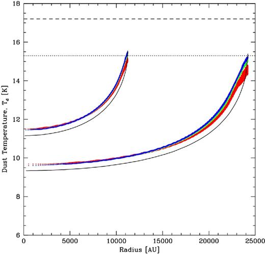
The dust temperature as a function of radius inside two uniform-density molecular cloud cores that are subject to an external ISR field. The clouds have the same densities, but different masses: 1 M_⊙ (upper distributions) and 10 M_⊙ (lower distributions). The exact solutions are plotted using the solid black lines. For the SPH calculations, a point is plotted for each SPH particle (2.6 × 10⁵ for each cloud). The different colours give the results obtained when the code uses 12 (red), 48 (green), or 192 (blue) healpix directions to calculate the mean extinction. Dust within the clouds receives less of the external radiation due to extinction and, therefore, is colder. The number of healpix directions used has little impact on the results, except in the very outer part of the clouds. The equilibrium temperature of dust that is subject to the full ISR is 17.2 K (horizontal dashed line), and the equilibrium temperature of dust that received exactly half of this radiation would be 15.3 K, which is lower by a factor of 2^1/6 (horizontal dotted line). As expected, dust at the edges of the clouds is close to this temperature.

Open in new tab Download slide

In Fig. 3, we plot the dust temperatures from five calculations of the 1-M_⊙ cloud that each use 48 healpix directions, but that have different numbers of SPH particles: 280, 2608, 2.6 × 10⁴, 2.6 × 10⁵, and 2.6 million. It can be seen that the dust temperature tends to be overestimated when a smaller number of particles is used, but the dust temperature appears to be slowly converging towards the exact solution as the number of particles is increased. The error in the dust temperature is approximately halved each time the number of SPH particles is increased by an order of magnitude (i.e. the error decreases at about the same rate that the linear spatial resolution increases). Comparing the 2.6 × 10⁴ particle calculation with the exact solution, the maximum difference between the mean temperatures at any radius is only 1 K. Clark et al. (2012a) did not discuss how their method behaves with different numbers of particles.

Figure 3.

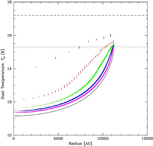
The dust temperature as a function of radius inside the 1 M_⊙ uniform-density molecular cloud core that is subject to external ISR. The exact solution is plotted using the solid black line. The results from five SPH calculations are illustrated, and a point is plotted for each SPH particle. The calculations each use 48 healpix directions to calculate the mean extinction, but different numbers of SPH particles are used to model the cloud – from top to bottom: 280 (black), 2608 (red), 2.6 × 10⁴ (green) 2.6 × 10⁵ (blue), and 2.6 million (magenta). It can be seen that using fewer particles tends to result in warmer dust temperatures (i.e. an underestimate of the extinction), but the dust temperature appears to be slowly converging towards the exact solution as the number of particles is increased. As long as ≳3 × 10⁴ particles are used the maximum error in the mean temperature at any radius is ≲ 1 K. The equilibrium temperature of dust that is subject to the full ISR is 17.2 K (horizontal dashed line), and the equilibrium temperature of dust that received exactly half of this radiation would be 15.3 K, which is lower by a factor of 2^1/6 (horizontal dotted line). As expected, with sufficient resolution, the dust at the edges of the clouds is close to this temperature.

Open in new tab Download slide

We used a cubic lattice SPH particle distribution to generate the results presented in Figs 2 and 3. We have also tried a random particle distribution. Using 2.6 × 10⁵ randomly-placed SPH particles to model the 1-M_⊙ cloud, we obtained an almost identical mean radial temperature distribution to the case that used a cubic lattice, but with a temperature scatter of up to ±0.2 K. However, given that this error is similar to the systematic difference between the temperature distributions obtained from the 2.6 × 10⁵ and 2.6 million particle cubic lattice calculations, we conclude that the accuracy of the solution depends more on the number of particles used than on the details of how they are distributed.

In Fig. 4, we investigate the effects on the calculation of the dust temperature of varying the tree-opening criterion and the effective radius of the tree nodes, the latter of which is parametrized by the factor f (see Section 3.1.2). During the walk through the tree to calculate gravity, nodes are opened if s_n/r_np is larger than a critical value, usually taken to be 0.5. We perform calculations using a tree-opening parameter of 0.5 and 0.25 (the latter of which means more nodes are opened during the tree walk). For each case, we perform five SPH calculations of the 1-M_⊙ cloud that each use 48 healpix directions and 2.6 × 10⁵ SPH particles, but we vary the effective radius of the node that is used when calculating the column density. We take factors of f = 2.0, 1.0, 0.5, 0.1, and 0.01. It can be seen from Fig. 4 that using very large tree-opening angles and/or effective node radii results in warmer dust temperatures (i.e. an underestimate of the extinction). We also note that almost identical results are obtained when the product of the opening parameter and the factor f is a constant (e.g. using a tree-opening parameter of 0.5 and f = 1 gives almost identical results to using a tree-opening parameter of 0.25 and f = 2). The calculation of the extinction becomes very poor when the product of these two quantities exceeds ≈0.5. If the effective node size is too small, the calculations provide reasonable mean temperatures at a given radius, but the scatter increases (e.g. the black points in the left-hand panel that were produced using f = 0.01). With the typical tree-opening parameter of 0.5, setting the factor f = 0.5 gives the best trade-off between accurately computing the mean radial temperature distribution and minimizing the scatter.

Figure 4.

The dust temperature as a function of radius inside the 1 M_⊙ uniform-density molecular cloud core that is subject to external ISR. The exact solution is plotted using the solid black line. The results from 10 SPH calculations are illustrated, and a point is plotted for each SPH particle. The calculations each use 48 healpix directions to calculate the mean extinction and 2.6 × 10⁵ SPH particles, but the tree-opening parameter and the effective sizes of the tree nodes are varied. In the left-hand panel, the tree-opening parameter is 0.5, while in the right-hand panel it is 0.25. In each panel, the effective size of the tree nodes decreases from top to bottom, using scaling factors of f = 2.0 (red), 1.0 (green), 0.5 (blue), 0.1 (magenta), and 0.01 (black). It can be seen that using very large tree-opening angles and/or effective node sizes results in warmer dust temperatures (i.e. an underestimate of the extinction). If the effective node size is too small, the scatter increases. With a tree-opening parameter of 0.5, an effective node size of half the actual node size (i.e. f = 0.5) gives the best trade-off between accurately computing the mean radial temperature distribution and minimizing the scatter. The equilibrium temperature of dust that is subject to the full ISR is 17.2 K (horizontal dashed line), and the equilibrium temperature of dust that received exactly half of this radiation would be 15.3 K, which is lower by a factor of 2^1/6 (horizontal dotted line). As expected the dust right at the edges of the clouds is close to this temperature.

Open in new tab Download slide

The typical resolutions employed in SPH calculations of star cluster formation vary from ∼10³ particles per solar mass (Bonnell, Bate & Vine 2003; Bonnell et al. 2011) to ∼10⁵ particles per solar mass (Bate, Bonnell & Bromm 2003; Bate 2012). The results of this test suggest that the typical errors in the dust temperature due to finite numbers of SPH particles and healpix directions and variations of the tree parameters should be ≲1 K as long as ≳3 × 10⁴ particles per solar mass are used and large effective node radii are avoided.

4.2 Equilibrium dust and gas temperatures

More realistic than using a uniform-density sphere is to use Bonner–Ebert spheres. To allow comparison with earlier work, we use the same 5-M_⊙ Bonner–Ebert spheres that were used by Keto & Field (2005) – a (marginally) subcritical case with a central density of n_H2 = 10⁴ cm⁻³, and a supercritical case with a central density of n_H2 = 10⁶ cm⁻³. The former case has a ratio of the inner to outer density of 14, while the ratio of the latter is 3000. Their radii are 0.223 and 0.265 pc, respectively. In these tests, we assume the hydrogen is fully molecular. We model both clouds with 3 × 10⁵ SPH particles.

The SPH particles were set up using a cubic lattice which was then deformed radially to obtain the required cumulative radial mass profile. In Fig. 5, we provide the SPH density as a function of radius for of each SPH particle for both cores. The small ‘spikes’ in the density in the supercritical case are due to the lattice structure affecting the density calculation of some particles in this case with a very strong density gradient. They do not appear in the subcritical case, which has a much shallower density profile. In both cases, there is also some ‘noise’ in the density near the outer boundary (which is made of reflected ghost particles).

Figure 5.

Plots of the SPH molecular hydrogen number density, n_H2, as functions of radius inside the subcritical (blue) and supercritical (red) 5-M_⊙ Bonner–Ebert spheres. A point is plotted for each SPH particle. The ‘spikes’ in the density for the supercritical case are an artefact of the particles being set up on a radially-deformed cubic lattice.

Open in new tab Download slide

In this section, we investigate the effects of each of the physical heating and cooling mechanisms on the temperatures of the gas and dust. We begin by including only cosmic ray heating and molecular line cooling for the gas, and the dust is taken to be in thermal equilibrium with the ISR. We then add in the effects of gas–dust collisions, photoelectric heating of the gas and cooling from C⁺. For the first two cases, we also investigate the effects of including and excluding the UV flux.

4.2.1 Cosmic ray heating, molecular line cooling, and dust radiative equilibrium

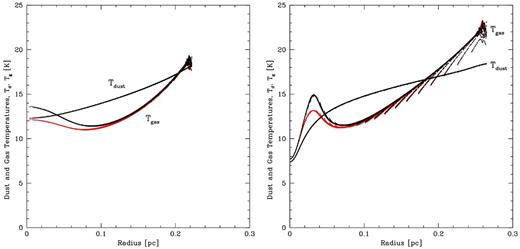
In Fig. 6, we plot the dust and gas temperatures as functions of radius inside the two Bonner–Ebert spheres. These calculations include only cosmic ray heating and undepleted molecular line cooling of the gas, and the dust is in thermal equilibrium with the external ISR. There is no gas–dust collisional coupling, photoelectric effect, or cooling due to C⁺, oxygen, or recombination lines. There are two calculations for each case – one that excludes the UV contribution to the ISR, and one that includes it.

Figure 6.

The dust (upper) and gas (lower) temperatures as functions of radius inside the subcritical (left) and supercritical (right) 5-M_⊙ Bonner–Ebert spheres. The ISM physics includes cosmic ray heating and molecular line cooling of the gas, and the dust is in thermal equilibrium with an external ISR that excludes (green) or includes (red) the UV contribution (see Section 2.4.1). The dust temperature drops as the extinction increases at smaller radii. The gas temperature rises because the line cooling becomes less effective at higher densities. The UV ISR only affects the dust temperature in the low-extinction outer parts of the cloud. The small ‘spikes’ in the gas temperature in the right plot at radii r ≈ 0.03–0.16 pc are due to the artefacts in the calculation of the SPH density due to the particles being set up on a radially-perturbed cubic lattice.

Open in new tab Download slide

In the outer parts of the cores, the dust temperature exceeds the gas temperature as the local ISR is only weakly attenuated by the dust, and the cosmic ray flux and line cooling are such that the low-density equilibrium gas temperature is ≈10 K. Including the UV contribution to the ISR boosts the dust temperature by up to 2 K in the outer parts, but the total energy in the UV flux is small compared to the total ISR flux and the UV does not penetrate very far into the cores. In the inner parts of the cores, the gas temperature rises as the effectiveness of the line cooling decreases (Goldsmith 2001). On the other hand, the dust temperature decreases, particularly in the supercritical case, because the dust extinction attenuates the ISR.

4.2.2 The effects of gas–dust collisions

In Fig. 7, we include the same physical processes as in the previous section, but we now also turn on the transfer of thermal energy between the gas and the dust due to collisions. The strength of this interaction depends on the square of the density (equation 36), so we expect it to have little impact at low densities, but a significant impact as the density increases. Indeed, this can be clearly seen in Fig. 7, in which we plot the same calculations as in Fig. 6 for reference, but we now also include the case with gas–dust coupling in blue (without the UV ISR) and magenta (with the UV ISR). The gas–dust thermal coupling has no significant effect on the temperatures in the subcritical core because the densities are too low. In the supercritical case, the dust temperature is unaffected, but the gas temperature at r < 0.04 pc (densities n_H2 ≳ 2 × 10⁴) is ‘dragged down’ by the interaction with the cold dust so that at the centre the gas and dust temperatures are both ≈7.5 K.

Figure 7.

The dust (upper) and gas (lower) temperatures as functions of radius inside the subcritical (left) and supercritical (right) 5-M_⊙ Bonner–Ebert spheres. Red and green points (mostly obscured) are the same as in Fig. 6. For the blue (without the UV ISR) and magenta (with the UV ISR) points, the ISM physics is exactly the same, except that it includes thermal collisional coupling between the gas and the dust. The black solid lines give the results obtained by Keto & Field (2005) without including the UV ISR. The effect is that at high densities, the gas essentially adopts the dust temperature. The small ‘spikes’ in the gas temperature in the right-hand plot at radii r ≈ 0.03–0.16 pc are due to the artefacts in the calculation of the SPH density due to the particles being set up on a radially-perturbed cubic lattice.

Open in new tab Download slide

Our numerical results are in reasonable agreement with those presented in figs 4 and 5 of Keto & Field (2005), who use the same models for the ISM physics as we use here, without the UV ISR (black solid lines in Fig. 7). The main difference is that the gas temperatures at low densities are slightly lower in Keto & Field (2005). The gas temperature at low density is set by the balance between cosmic ray heating and the line cooling rates. The latter is dependent on the method used to interpolate from the tables of Goldsmith (2001). Since the cosmic ray heating and line cooling rates are both simple functions of n_H (equations 24 and 34), it is easy to solve for the central gas temperature of 12.4 K in the subcritical case (where the gas–dust coupling is negligible). The slightly lower gas temperature (≈11.5 K) obtained by Keto & Field (2005) was found to be due to less accurate interpolation used by Keto & Field of the line cooling functions of Goldsmith (2001). Thus, the different interpolation of the line cooling produces the different gas temperatures.

4.2.3 The effects of photoelectric heating and carbon chemistry

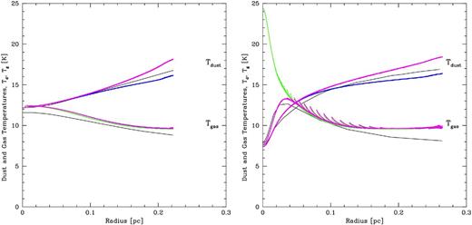
In Fig. 8 , in addition to the other physical processes, we turn on photoelectric heating of the gas due to UV ISR photons liberating electrons from dust grains (equation 26). The resulting gas and dust temperatures (green) are compared to those without the photoelectric heating (blue). The dust temperature is essentially unchanged, but the gas temperature in the outer parts of the cores, at densities such that the gas and dust are thermally decoupled (n_H2 ≲ 10⁴ cm⁻³), is much hotter than without photoelectric heating. In fact the photoelectric heating is so strong that the cosmic ray heating is irrelevant in the low-density gas.

Figure 8.

The effect of photoelectric heating and C⁺ cooling of the gas on the dust and gas temperatures as functions of radius inside the subcritical (left) and supercritical (right) 5-M_⊙ Bonner–Ebert spheres. The dust temperatures are essentially unaffected by the extra gas heating and cooling processes. The blue points are the same as in Fig. 7, where the gas is subject to cosmic ray heating, molecular line emission, and collisions with the dust, while the dust is subject to heating from the ISR (including the UV), thermal emission, and collisions with the gas. The green points include the same physical effects as the blue points, but with the addition of photoelectric gas heating (equation 26). The photoelectric heating has an enormous effect on the gas temperature in the outer, low-density parts of the clouds. However, when the C⁺ cooling is included (red points), the effect of the photoelectric heating on the gas temperature is greatly reduced.

Open in new tab Download slide

Whereas Keto & Field (2005) did not consider photoelectric heating, as discussed in Section 2.5, Keto & Caselli (2008) included photoelectric heating and a simple carbon chemistry model which allowed them to include both cooling from C⁺ at low densities and treat the depletion of CO at high densities. Therefore, in Fig. 8, we keep the photoelectric heating on, but also add cooling from C⁺ (red). It can be seen that the C⁺ cooling dramatically lowers the temperatures in the outer parts of the cloud; the temperature is still somewhat higher than it was without either the photoelectric heating or the C⁺ cooling, but much less than if C⁺ cooling is omitted. We note that recombination and oxygen cooling are both insignificant at these densities and that the temperatures are essentially identical whether they are included or not.

Finally, in Fig. 9 we turn on the effects of CO depletion based on the equilibrium prescription of Keto & Caselli (2008). This results in only slightly higher gas temperatures at intermediate densities (n_H2 = 10⁴–10⁵ cm⁻³) where the densities are still too low for dust cooling to dominate, but the densities are high enough that C⁺ is ineffective.

Figure 9.

The effect of CO depletion on the gas on the dust and gas temperatures as functions of radius inside the subcritical (left) and supercritical (right) 5-M_⊙ Bonner–Ebert spheres. The red points are the same as in Fig. 8, where the gas is subject to cosmic ray and photoelectric heating, molecular and C⁺ line emission, and collisions with the dust, while the dust is subject to heating from the ISR (including the UV), thermal emission, and collisions with the gas. The black points include the same physical processes as the red points, but also allow for CO depletion. This reduces the molecular line cooling at high densities which raises the gas temperature slightly at densities n_H2 = 10⁴–10⁵ cm⁻³. At higher densities the depletion has little effect because the cooling is dominated by dust emission through collisions with the dust.

Open in new tab Download slide

4.2.4 The effects of changing the ISM parameters

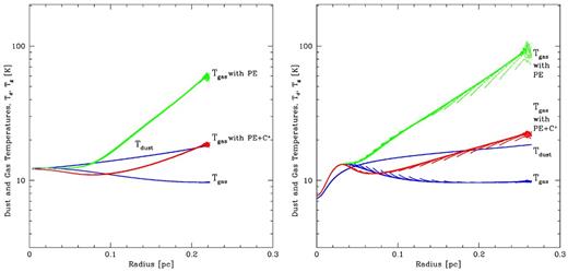
The previous sections used the diffuse ISM model parameters described in Sections 2.3 and 2.4. In this section, we investigate the dependence of the gas and dust temperatures on the strengths of the various external heating sources. We only use the supercritical Bonner–Ebert sphere in these tests because this has the larger range of densities. In the left-hand panel of Fig. 10, we explore the effects of changing the cosmic ray heating rate (equation 24) by an order of magnitude in each direction. In the right-hand panel of Fig. 10, we explore the effects of change the gas photoelectric heating rate (equation 26) by an order of magnitude in each direction. It can be seen that over particular density ranges, either of these changes the gas temperature by approximately half an order of magnitude in each direction because the gas line cooling scales roughly as the square of the gas temperature for the molecular lines (Goldsmith 2001). The gas temperatures in the outer parts of the cloud are much more strongly affected by photoelectric heating than cosmic ray heating. On the other hand, at number densities n_H2 ≳ 10⁵ cm⁻³ strong cosmic ray heating can raise the gas temperature significantly above the dust temperature whereas the photoelectric heating has no effect this deep within the core.

Figure 10.

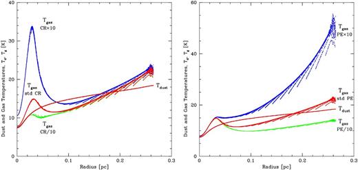
The effects of changing the strengths of the cosmic ray (left) and photoelectric (right) heating of the gas on the dust and gas temperatures as functions of radius inside the supercritical 5-M_⊙ Bonner–Ebert sphere. In both panels, the red points are the same as in the black points in the right-hand panel of Fig. 9. The other points include the same physical effects as the red points, but with one order of magnitude less (green) or more (blue) cosmic ray (left) or photoelectric (right) heating. Changing the level of cosmic ray heating has a large effect on the gas temperature at intermediate densities, but not at high densities (where the gas and dust are well coupled) or low densities (where photoelectric heating dominates). Changing the levels of photoelectric heating has a large effect on the gas temperature only in the outer regions of the core. The dust temperatures are unaffected in either case.

Open in new tab Download slide

In Fig. 11, we probe the effects of changing the ISR field (equation 25) by an order of magnitude in each direction, excluding the UV contribution which is held fixed. The calculations include photoelectric heating of the gas and C⁺ cooling. The increased ISR primarily affects the dust temperature, but because the dust emission scales as the sixth power of its temperature (equation 23), this only has a 50 per cent effect on the dust temperatures. Deep within the core where the gas becomes thermally coupled to the dust, the warmer or cooler dust also results in warmer or cooler gas, respectively.

Figure 11.

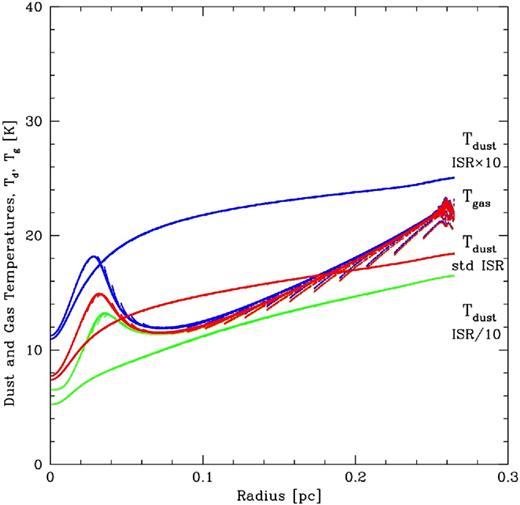
The effects of changing the strength of the ISR field on the dust and gas temperatures as functions of radius inside the supercritical 5-M_⊙ Bonner–Ebert sphere. The red points are the same as the black points in the right-hand panel of Fig. 9. The other points include the same physical effects as the red points, but with one order of magnitude less (green) or more (blue) ISR heating. Changing the level of ISR by an order of magnitude has a 50 per cent effect (10^1/6) on the dust temperatures. At high densities, the different dust temperature affects the gas temperature in a similar manner, but at low densities the gas temperature is unaffected as it is set by the photoelectric heating and C⁺ cooling.

Open in new tab Download slide

In Fig. 12, we investigate the effects of changing the metallicity of the core, performing additional calculations with metallicities of 1 per cent, 10 per cent, and 3 times solar. It can be seen that the highest metallicity results in the coldest temperatures for both the gas and the dust due to the combination of several effects. The increased metallicity increases the ISR attenuation, decreasing the dust temperature inside the core. Similarly, the UV is prevented from penetrating as far into the core, reducing the effects of photoelectric heating of the gas, and the gas line emission is enhanced. Finally, there is an increase in the effectiveness of collisional thermal coupling between the gas and the dust. With the lowest metallicity, the dust almost becomes isothermal since there is almost no attenuation of the ISR, and the gas is warmer because the photoelectric heating is strong while emission line cooling is weak.

Figure 12.

The effects of changing the metallicity on the dust and gas temperatures as functions of radius inside the supercritical 5-M_⊙ Bonner–Ebert sphere. Photoelectric heating has been included. From top to bottom, the calculations have metallicities of 1/100 (magenta points, top curves), 1/10 (blue points), solar metallicity (red points), and 3 times solar metallicity (green points). The red points are the same as in the black points in the right-hand panel of Fig. 9. The dust temperatures are greater with lower metallicities because the ISR is less attenuated by extinction. The gas temperatures are greater with lower metallicities because the UV ISR is less attenuated by extinction (leading to stronger photoelectric heating) and also because the gas emission line cooling is reduced.

Open in new tab Download slide

4.3 The evolution of a collapsing Bonner–Ebert sphere

In this section, as opposed to the static tests from the previous sections, we report the results from a hydrodynamical calculation of the collapse of a Bonner–Ebert sphere and compare them to the results obtained using the pure flux-limited diffusion method of Whitehouse et al. (2005) and Whitehouse & Bate (2006). We begin with a somewhat unstable Bonner–Ebert sphere, similar to those studied in the previous section. We choose a 5-M_⊙ core with an inner to outer density contrast of 20 and a radius of 0.1 pc. We model the core with 3 × 10⁵ SPH particles and use spherical reflective boundary conditions (modelled using ghost particles).

In Fig. 13, we plot the central temperatures as functions of the central (maximum) density for the two methods. All of the initial temperatures in the pure flux-limited diffusion calculations are arbitrary. As is standard practice in such calculations, we set the matter and radiation temperatures to be in thermal equilibrium initially. We perform two separate calculations and with two different initial temperatures of 10 and 14 K. For the calculation performed using the method described in this paper, the initial gas and dust temperatures are not arbitrary – they are set by our model of the diffuse ISM. The initial dust temperature increases from 8 K in the centre to 17 K at the outer edge of the molecular cloud core. The initial gas temperature is slightly warmer than the dust at the centre (10 K) and cooler at the outside (≈15 K). The initial central dust and gas temperatures are quite similar because the central density of the core is quite high (ρ = 6 × 10⁻¹⁹ g cm⁻³ or n_H2 = 1.5 × 10⁵ cm⁻³) so that there is significant thermal coupling between the dust and the gas (we use equation 36 in these calculations). As the collapse proceeds, the central dust and gas temperatures quickly converge, so we do not plot the central dust temperature in Fig. 13. The increases in extinction and density during the collapse mean that both the dust and gas temperatures drop to a minimum of 6.5 K when the central density is 10⁻¹⁶ g cm⁻³ before the compressional heating starts to increase the central temperature again. The initial radiation temperature should be set to a low value, because the heating of the initial conditions is via external radiation rather than internal radiation. As long as a small value is chosen the exact value is unimportant, but we wish to avoid setting it to zero so as to avoid numerical problems. We chose a value of 1 K.

Figure 13.

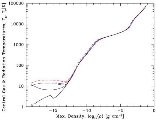
The evolution of the central gas and radiation temperatures as functions of the maximum (central) density during a radiation hydrodynamical calculation of the collapse of an unstable spherical 5-M_⊙ Bonner–Ebert sphere. The radiation temperature is always less than or equal to the gas temperature in this graph. After the central density exceeds 10⁻¹⁷ g cm⁻³, the central dust temperature is indistinguishable from that of the gas. The black solid lines give the results from a calculation using the method described in this paper, while the red dashed lines and blue long-dashed lines give the results using the pure FLD method of Whitehouse & Bate (2006). The diffuse ISM model used in the former calculation determines the initial gas and dust temperatures, which vary with radius, and the internal radiation temperature is arbitrarily set to a low initial value (1 K). In the FLD calculations, the initial temperatures of the matter (gas and dust) and internal radiation are arbitrary and we set them to 14 K (red dashed) and 10 K (blue long-dashed). As expected, it is mainly the low-density evolution that is affected by including the diffuse ISM model.

Open in new tab Download slide

As may be expected, Fig. 13 shows that it is mainly the low-density phase of evolution of the clouds that differs between the two methods (densities ≲10⁻¹³ g cm⁻³). Once the central regions of the core become optically-thick to infrared radiation (the so-called opacity limit for fragmentation; Low & Lynden-Bell 1976; Rees 1976) all of the temperatures converge. The evolution obtained with the pure flux-limited diffusion calculation with the lower initial temperature (10 K) is closest to the evolution obtained using the method presented here, presumably because the central temperature in this model is closest to that given by the ISM initial conditions.

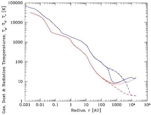
In Fig. 14, we plot temperature profiles as functions of radius (left-hand panel) and density (right-hand panel) at various points during the collapse. Gas is shown with solid lines, dust with dotted lines, and radiation with dashed lines. At either a given radius or density the temperatures tend to rise during the collapse as the protostar emits more radiation. The formation of the stellar core at late times (initial radius ≈0.01 au and temperature >10⁴ K) is clearly visible in the left-hand panel. Except in the outer parts of the core, these profiles are very similar to those obtained using pure flux-limited diffusion. The main difference in the outer parts of the core (radii ≳10³ au) is that the gas, dust, and radiation all have different temperatures with the new method, whereas with pure flux-limited diffusion all are very close to the initial arbitrary temperature (e.g. 10 K; see Whitehouse & Bate 2006).

Figure 14.

The evolution of the gas (solid), dust (dotted), and radiation (dashed) temperatures as functions of radius (left-hand panel) and maximum density (right-hand panel) during a radiation hydrodynamical calculation of the collapse of an unstable spherical 5-M_⊙ Bonner–Ebert sphere. Each colour gives the state of the calculation when the maximum density reaches a different value, with the initial conditions given in black. The radiation temperature is always less than or equal to the gas temperature in this graph. The thick black long-dashed lines in the right-hand panel give the evolution of the central gas and radiation temperatures with central density from Fig. 13 for reference (only for ρ > 10⁻¹⁵ g cm⁻³). It can be seen that for a given density the gas is usually hotter latter in the collapse than earlier due to radiation from the protostar heating the outer parts of the core. The formation of the stellar core is apparent in the upper-left of the left-hand panel (initial radius ≈0.01 au).

Open in new tab Download slide

After stellar core formation as radiation works its way outwards from the centre the gas, dust, and radiation temperatures become inverted at intermediate radii in the core (radii 400–3000 au; Fig. 15). Before this point the gas temperature is the hottest and the radiation temperature the coldest at these radii. However, the radiation emitted by the protostar quickly dominates that from the external radiation field at these radii. The dust adopts a new thermodynamic equilibrium with the combined radiation field, being heated to temperatures of 15–40 K, but the gas which is poorly coupled to either the radiation or the dust at these low densities remains at temperatures of 8–12 K. Such effects are impossible to capture unless the thermal evolution of the gas and dust are treated separately.

Figure 15.

The gas (solid), dust (dotted), and radiation (dashed) temperatures as functions of radius when the collapsing spherical 5-M_⊙ Bonner–Ebert sphere has reached a maximum density of 0.01 g cm⁻³ (lower, red lines), and 1.76 years later at the end of the calculation when the maximum density is 0.06 g cm⁻³ (upper, blue lines). Near the end of the calculation, after the stellar core forms, the radiation and dust temperatures become hotter than the gas temperature at radii of 400–3000 au because of the radiation emitted by the protostar.

Open in new tab Download slide

4.4 The evolution of an isolated turbulent molecular cloud

Glover & Clark (2012a,c) studied the thermodynamics of turbulent molecular clouds with different metallicities. In particular, they performed calculations of 10⁴ M_⊙ clouds, typically modelled using SPH with 2 million particles. Their initial conditions consisted of a uniform-density sphere of number density n_H = 300 cm⁻³, giving a radius of approximately 6 pc. The cloud was given initial ‘turbulent’ motions with a power spectrum P(k) ∝ k⁻⁴, where k is the wavenumber. The energy in the turbulence was initially set equal to the magnitude of the gravitational potential energy of the cloud, giving an initial root-mean-square velocity of around 3 km s⁻¹. The turbulence was allowed to decay freely. The calculations were performed using a confining pressure of p_ext = 1.2 × 10⁴ K cm⁻³ which was implemented in the SPH equations by subtracting the external pressure from the pressure used in the momentum equation. We use the same set up as Glover & Clark, although of course we are unable to use exactly the same initial velocity field. We use our full diffuse ISM model to obtain the results below, but we begin by excluding the hydrogen chemistry and heating due to the formation of molecular hydrogen (Section 2.5.2). In the first set of results, we have also excluded molecular depletion (because Glover & Clark did not include depletion), but since we find that switching depletion on or off has little effect on the results it is included in most of the subsequent calculations. For the dust–gas thermal coupling, we switch to equation (37) because this is the equation Glover & Clark used.

4.4.1 Results excluding hydrogen chemistry

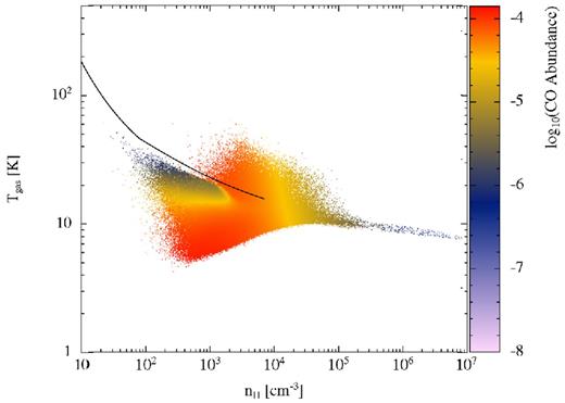
In Fig. 16, we plot the gas (upper panel) and dust (lower panel) temperatures as functions of the number density of hydrogen nuclei, n_H, for a calculation performed at solar metallicity. The snapshot is taken just before the first sink particle is formed. The colours in the gas temperature plot indicate the average CO abundance of each point in temperature–density space. This is the equivalent of fig. 2 in Glover & Clark (2012a) or the upper-right panel of Fig. 4 in Glover & Clark (2012c). Since Glover & Clark did not include molecular depletion on to grains, we have turned this off in our calculation. The distribution of gas temperatures with density shows the same general features seen in the papers of Glover & Clark. At low densities (n_H ≲ 10³ cm⁻³), the gas temperature rises towards ∼100 K as the number density decreases towards n_H ∼ 10 cm⁻³. The temperatures at densities n_H ≲ 100 cm⁻³ are primarily determined by the models of photoelectric heating, and cooling due to electron recombination and emission from ionized oxygen and carbon (equations 26 to 33). The gas temperatures lie beneath the equilibrium curve (solid black line from Fig. 1) because the equilibrium curve assumes no extinction whereas in fact the photoelectric heating is generally attenuated by the dust extinction (depending on the location of the gas). Our maximum temperatures in this density regime are somewhat cooler than those obtained by Glover & Clark due to our slightly different models in this regime as already demonstrated in Fig. 1. At densities n_H ≈ 100–10⁴ cm⁻³, there is a large dispersion in the gas temperatures with a range of T_g ≈ 8–50 K obtained at densities n_H ≈ 10³–10⁴ cm⁻³. In this region, although there is still significant photoelectric heating, the low-density coolants just mentioned become ineffective. Instead, the main cooling is from molecular lines, in particular CO (e.g. Goldsmith 2001; Glover & Clark 2012a), which depends strongly both on density and temperature. At the same time, work from the gas motions becomes important (either heating or cooling the gas, depending on whether the gas is being compressed or expanding, respectively), as does heating in shocks. Together these effects lead to the wide range in temperatures. Finally, at densities n_H ≳ 10⁵ cm⁻³ thermal coupling of the gas to the dust becomes important and the gas temperature converges towards that of the dust as the density increases.

Figure 16.

Phase diagrams showing the gas (top panel) and dust (lower panel) temperatures as functions of the gas density. The colours in the gas temperature plot indicate the average CO abundance of each point in temperature–density space. The black solid line in the gas temperature plot is the equilibrium curve from Fig. 1.

Open in new tab Download slide

As mentioned above, Glover & Clark (2012a) do not treat depletion of CO on to dust grains. Turning this on has little effect on the phase diagram (Fig. 17). As may be expected, the temperatures at densities of n_H ≈ 10³–10⁵ cm⁻³ are slightly higher, but the effect is hardly noticeable. At lower densities the CO is not depleted and the dominant coolant is C⁺ rather than CO anyway. At higher densities where the CO does become depleted, the dominant coolant is dust.

Figure 17.

Phase diagram showing the gas temperature as a function of the gas density for a calculation that is identical to that portrayed in Fig. 16, except that molecular depletion is turned on. The black solid line is the equilibrium curve from Fig. 1.

Open in new tab Download slide

We now explore the sensitivity of the results to several of the assumptions in our model. We examine the dependence on changes of the chemistry, in particular the abundance of C⁺ and the depletion of molecules like CO on to grains, as well as the effects of variations in the molecular line cooling rates and the strength of the coupling between the gas and the dust.

The main effect of the carbon chemistry model described in Section 2.5.1 is to provide the abundances of the coolants C⁺ at low-densities and CO at high densities. Typically, the transition between the dominance of the two coolants occurs at n_H ∼ 10³ cm⁻³ (e.g. Glover & Clark 2012a). The temperature of the gas is quite sensitive to this transition from C⁺ to CO. For example, in Fig. 18 we give the results obtained by assuming that the carbon remains as C⁺ at all densities and we turn off all molecular cooling. In this case, essentially all of the gas lies at temperatures below the equilibrium curve of Fig. 1 and there is little gas with temperatures greater than 20 K with densities n_H ≈ 10³–10⁵ cm⁻³. This extreme case shows that it is important to have at least a simple model that switches the carbon from C⁺ to CO.

Figure 18.

Phase diagram showing the gas temperature as a function of the gas density for a calculation that is identical to that portrayed in Fig. 17, except that all the carbon is assumed to be in the form of C⁺. The black solid line is the equilibrium curve from Fig. 1.

Open in new tab Download slide

In Fig. 19, we return to our standard model including molecular depletion, but we increase the molecular line cooling rates by an arbitrary factor of 3. As expected, this decreases the temperatures of the gas with densities n_H ≈ 10³–10⁵ cm⁻³. The lowest temperature (at densities n_H ≈ 10³ cm⁻³) decrease from T_g ≈ 8 to ≈5 K, but the highest temperatures (at densities n_H ≈ 10³ cm⁻⁴) are not significantly affected.

Figure 19.

Phase diagram showing the gas temperature as a function of the gas density for a calculation that is identical to that portrayed in Fig. 17, except that the molecular line cooling rate has been increased by a factor of 3. The colours in the gas temperature plot indicate the CO abundance of each point in temperature–density space. The black solid line is the equilibrium curve from Fig. 1.

Open in new tab Download slide

As mentioned in Section 2.4.3, equations (36) and (37) for the gas–dust thermal coupling coefficient differ by a factor of 15 (the latter, used by Glover & Clark, gives stronger coupling). Therefore, in Fig. 20 we examine the effect of using the weaker coupling provided by equation (36) instead. As expected, this only has an effect on the temperatures at high densities, n_H ≳ 10⁵ cm⁻³. The gas shows a somewhat increased spread of temperatures because the coupling with the dust is not strong enough to force the gas to adopt the dust temperature.

Figure 20.

Phase diagram showing the gas temperature as a function of the gas density for a calculation that is identical to that portrayed in Fig. 17, except that the collisional thermal coupling between the dust and the gas is 15 times smaller (equation 36 has been used rather than 37). Note that there is a larger dispersion in the gas temperatures at densities n_H ≳ 10⁵ cm⁻³. The black solid line is the equilibrium curve from Fig. 1.

Open in new tab Download slide

In summary, the gas temperatures in solar metallicity turbulent clouds are relatively independent of many of the parameters of our diffuse ISM model. The most important factors are the low-density equilibrium model (portrayed in Fig. 1) which essentially sets an upper limit to the temperatures at densities n_H ≲ 10³ cm⁻³, and the way in which the carbon transitions from C⁺ to CO. The exact molecular cooling rates, molecular depletion, and dust–gas thermal coupling parameters are less important.

4.4.2 The effects of metallicity and hydrogen chemistry

Following Glover & Clark (2012c), we examine the dependence on metallicity and on hydrogen chemistry. We perform full calculations (i.e. including the simple carbon chemical model and molecular depletion) for four different metallicities: 3, 1, 1/10, and 1/100 times the solar value. For each metallicity, we perform calculations that exclude hydrogen chemistry and its associated heating terms (results from the solar metallicity case have already been displayed in Fig. 17). We also perform calculations that include the evolution of hydrogen (i.e. its molecular fraction x_H2) and heating due to H₂ formation on dust grains. Two calculations are performed for each metallicity: one beginning with fully atomic hydrogen, and one beginning with fully molecular hydrogen.

In Fig. 21, we plot the evolution of the fractional abundance of molecular hydrogen in the eight calculations that include hydrogen chemistry up until the formation of the first sink particle in each calculation. This is the equivalent of fig. 3 in Glover & Clark (2012c). Beginning with fully molecular hydrogen, the decrease in H₂ is primarily due to photodissociation in the outer parts of the clouds. The destruction is greater at lower metallicities because the UV radiation is less attenuated by dust. Beginning with fully atomic hydrogen, H₂ is formed on dust grains and the total abundance monotonically increases in each calculation. However, the rate of increase strongly depends on the metallicity. The main reason for this is that there are more dust grains on which to produce H₂ at higher metallicity (equation 40) so the rate of formation is higher. In addition, the extra dust attenuates the UV radiation that destroys H₂ so the destruction rate is also lower. By the time stars begin to form, clouds with solar metallicity or higher are mostly molecular regardless of whether atomic or molecular initial conditions were adopted (particularly in the central regions where the stars actually form). However, at lower metallicities the initial conditions matter much more. When stars begin to form in the 1/10Z_⊙ calculations, the H₂ abundance is 65 per cent when beginning with molecular initial conditions, but only 15 per cent beginning with atomic initial conditions. For 1/100Z_⊙, the disparity is even stronger, with the two abundances being 60 and 1.7 per cent, respectively.

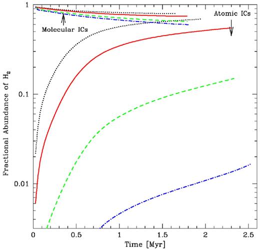
$We plot the evolution of the total fractional abundance of molecular hydrogen in calculations of turbulent clouds up until the time that stars begin to form. For each metallicity, we perform two calculations: one with fully molecular initial conditions (upper lines) and one with fully atomic initial conditions (lower lines). The metallicities are 3 times solar (black dotted lines), solar (red solid lines), 1/10 solar (green dashed lines), and 1/100 solar (blue dot–dashed lines). By the time stars begin to form, clouds with solar or supersolar metallicity are mostly molecular, regardless of their initial H2 abundance, but little molecular gas has formed in the low-metallicity clouds that consist of fully atomic hydrogen initially.$

Figure 21.

We plot the evolution of the total fractional abundance of molecular hydrogen in calculations of turbulent clouds up until the time that stars begin to form. For each metallicity, we perform two calculations: one with fully molecular initial conditions (upper lines) and one with fully atomic initial conditions (lower lines). The metallicities are 3 times solar (black dotted lines), solar (red solid lines), 1/10 solar (green dashed lines), and 1/100 solar (blue dot–dashed lines). By the time stars begin to form, clouds with solar or supersolar metallicity are mostly molecular, regardless of their initial H₂ abundance, but little molecular gas has formed in the low-metallicity clouds that consist of fully atomic hydrogen initially.

Open in new tab Download slide

The behaviour of the molecular hydrogen evolution is qualitatively similar to that reported by Glover & Clark (2012c). In particular, the growth rate of molecular hydrogen in the atomic solar-metallicity calculation matches theirs to within 10 per cent, and the decay rates of the abundances in all of the molecular calculations are very similar. The clouds in Glover & Clark (2012c) take longer to begin forming stars (2.7–4.0 Myr rather than 1.7–2.6 Myr). This difference is most likely due to the different initial turbulent velocity field. With fully molecular initial conditions, because the stars take longer to form in the calculations of Glover & Clark (2012c), the H₂ abundances when the star formation takes place are lower. This is most important in the lowest metallicity case, where the total abundance is only ≈20 per cent when the star formation begins in the Glover & Clark (2012c) calculation, whereas it is 60 per cent in our calculation. There are also differences in the abundances of molecular hydrogen in the lower metallicity calculations with atomic initial conditions. The total H₂ abundances when beginning with fully atomic hydrogen remain low throughout both our calculations and those of Glover & Clark. However, at any particular time our abundance is twice that obtained by Glover & Clark (2012c) with 1/10Z_⊙ and it is about an order of magnitude higher for the 1/100Z_⊙ case until shortly before stars begin to form (when the abundances in both calculations are ≈1 per cent). No doubt some of this difference is due to the different velocity field and dust opacities used in the calculations, though it is not clear whether or not this explains all of the discrepancy.

Turning to the phase diagrams of gas temperature in Fig. 22, the general trends are again in agreement with those found by Glover & Clark (2012c). First, we consider the calculations that exclude hydrogen chemistry (they assume all hydrogen is in molecular form) and its associated heating (left-hand column of Fig 22). Increasing the metallicity above solar results in a reduction of the lower envelope of the gas temperatures at densities n_H = 10²–10⁴ cm⁻³ because the additional molecular cooling and increased extinction produces lower gas temperatures. The upper temperature envelope is less affected. Lowering the metallicity to 1/10 of solar results in a smaller range of temperatures because extinction has less of an effect at low and intermediate densities so the temperatures tend to lie close to the equilibrium curve of Fig. 1 (which does not depend significantly on metallicity because the photoelectric heating and the cooling due to electron recombination and fine-structure emission are all assumed to be proportional to the metallicity). At higher densities, the main heating sources (compressional heating and cosmic ray heating) are independent of the metallicity and although the gas is less well coupled to the dust it is still coupled well enough that the gas temperatures are kept around 10 K. As the metallicity is reduced still further to 1/100 solar, the temperatures move above the solar metallicity equilibrium curve of Fig. 1. This is because the cosmic ray heating (which is taken to be independent of metallicity) becomes as important as the photoelectric heating at low metallicity. Furthermore, the magnitudes of the electron recombination and fine-structure cooling rates are proportional to metallicity, so regions that are heated by adiabatic and shock heating take longer to cool.

Figure 22.

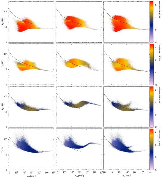
Phase diagrams of the gas temperature versus the gas density in turbulent clouds with metallicities of 3, 1, 1/10, and 1/100 times solar (top to bottom, respectively). The calculations in the left-hand column were performed without any H₂ chemistry (assuming purely molecular hydrogen) and without heating from H₂ formation. The other two columns included H₂ chemistry and heating from H₂ formation, but the calculations in the centre column began with fully atomic hydrogen, and the calculations in the right column began with fully molecular hydrogen. The colour bars indicate the average CO abundance of each point in temperature–density space (note that the scales differ from those in Figs 16, 17, 19, and 20). The black solid lines give the equilibrium curve from Fig. 1 for solar metallicity. Beginning with atomic gas results in significantly higher gas temperatures for densities n_H ∼ 10⁴–10⁶ cm⁻³ (or even higher densities in the low-metallicity cases) due to heating from H₂ formation on dust grains.

Open in new tab Download slide

At high densities n_H ≳ 10⁵ cm⁻³ where the gas is thermally coupled to the dust in the solar metallicity case there is not much change in the supersolar metallicity case. The temperatures are slightly cooler (about 1–2 K) because the coupling is even stronger and the dust has slightly cooler temperatures due to the increased extinction. A larger effect is seen with reduced metallicities because the thermal coupling to the dust is substantially weaker. At 1/10 solar metallicity, the gas has a maximum in the temperature distribution of about 15 K at n_H ≈ 3 × 10⁵ cm⁻³ before the dust cooling takes over and reduces the temperatures at higher densities. At 1/100 solar metallicity, the gas temperature rises with increasing density until n_H ≈ 2 × 10⁷ cm⁻³ when it reaches a maximum of ≈20 K before it begins to drop again at higher densities.

We now consider the effects of hydrogen chemistry on the gas temperature due to heating of the gas when molecular hydrogen is formed on dust grains (equation 50). This has little effect in the calculations that began with fully molecular hydrogen (right-hand column of Fig. 22). There are two small differences. First, in the solar and supersolar calculations the upper envelope of gas temperatures is higher at densities n_H ≈ 10²–10⁴ cm⁻³. This is because some molecular hydrogen is destroyed by photodissociation and when it reforms on dust grains this adds a source of heating. Second, in the low-metallicity calculations some regions of mostly atomic gas become molecular at densities n_H ≈ 10⁵–10⁶ cm⁻³ and the extra heating makes this gas hotter than the molecular gas at the same densities. Thus, a bifurcation of the gas temperature is apparent at these densities.

Beginning with fully atomic gas has a much greater effect on the gas temperature (centre column of Fig. 22). In these cases, heating due to H₂ formation on dust becomes significant at densities n_H ≳ 10³ cm⁻³, and the gas temperature is generally much greater than in the calculations without hydrogen chemistry or with fully molecular hydrogen initially. At solar and supersolar metallicities, the main effect is to raise the gas temperatures in the density range n_H ≈ 10³–10⁶ cm⁻³. Above these densities the gas is mostly molecular and the gas is thermally well-coupled to the dust. At low metallicities, the gas is significantly hotter from densities of n_H ≈ 10³ cm⁻³ even up to n_H ≈ 10⁸ cm⁻³. This is primarily because of the reduced dust abundance which has two main effects: the atomic hydrogen persists to higher densities, and the gas does not become thermally coupled to the gas until much higher densities.

As mentioned above, the general temperature trends seen here are in agreement with those found by Glover & Clark (2012c). However, there are also some differences. At low densities, our temperatures tend to be lower because of the different equilibrium models that we have already mentioned (Fig. 1). But there are also differences at higher densities. In the solar metallicity cases, Glover & Clark (2012c) obtain slightly lower minimum temperatures at n_H ∼ 10³ cm⁻³. This may be because their molecular cooling is somewhat stronger (cf. the difference that increasing the molecular cooling makes in Figs 17 and 19). In the calculations at 1/10 Z_⊙, the mean temperatures at each density are similar to those obtained by Glover & Clark (2012c) for both atomic and molecular initial conditions, but the scatter in the temperatures obtained by Glover & Clark (2012c) is greater at n_H ≳ 10⁵ cm⁻³. This may be largely due to the different density structure of the clouds (caused by the different initial velocity fields). In the lowest metallicity calculations (1/100 Z_⊙), the temperatures obtained by Glover & Clark (2012c) are generally higher than ours at n_H ≳ 10⁴ cm⁻³ for the molecular initial conditions, and above n_H ≳ 10⁶ cm⁻³ for the atomic initial conditions. This may be related to the higher molecular hydrogen abundances that were commented on when we discussed Fig. 21. In our initially atomic calculation, the gas is mostly molecular for densities n_H ≳ 10⁶ cm⁻³ meaning that there will be little heating from H₂ formation above these densities. If Glover & Clark (2012c) have more atomic gas remaining at high densities, this will provide additional heating. In our initially molecular calculation, because the stars begin to form at 2.0 Myr instead of 3.6 Myr, more of the initial molecular hydrogen remains. The total abundance is only 20 per cent in the calculation of Glover & Clark (2012c) when the temperature diagrams were plotted, whereas the total abundance in our calculation is 60 per cent and all of the high-density gas (n_H ≳ 10⁵ cm⁻³) is essentially fully molecular (i.e. there is little heating from H₂ formation). On the other hand, the temperature–density behaviour we obtain for the low-metallicity fully atomic initial conditions is in very good agreement with the results given in fig. 1 of Omukai et al. (2005). For 1/10 Z_⊙ calculations, the temperature at high densities has a peak at n_H ∼ 10⁵ cm⁻³ at similar temperatures in both our calculations and those of Omukai et al. At 1/100 Z_⊙, both our results and those of Omukai et al. display high-density temperature maxima of T_g ≈ 60 K at n_H ≈ 10⁶ cm⁻³.

5 CONCLUSIONS

We have presented a new method for modelling the thermal evolution of star-forming molecular clouds. The method combines a model for the thermodynamics of the diffuse ISM with radiative transfer in the flux-limited diffusion approximation. The former is required to correctly model the thermal behaviour of molecular clouds at low densities and metallicities, while the latter allows us to model protostar formation. Unlike most previously published star formation calculations, our new model evolves the temperatures of the gas, dust, and radiation separately. The code can also follow the evolution of atomic and molecular hydrogen. We have compared our method with existing literature on the thermal behaviour of the ISM and molecular cloud cores and generally obtain good agreement.

We have also explored the sensitivity of the thermal structure of molecular cloud cores and turbulent clouds to many of the parameters that enter our diffuse ISM model. For the gas at solar metallicities, the most important thermal processes at low densities (n_H ≲ 1–1000 cm⁻³) are photoelectric heating of electrons from dust grains and cooling due to electron recombination with small grains and PAHs and fine-structure emission from C⁺ and atomic oxygen. At high densities (n_H ≳ 10⁵ cm⁻³), cosmic ray heating and the work done by hydrodynamical flows dominate the heating, while the cooling is dominated by continuum dust emission so that the gas and dust adopt similar temperatures. At intermediate densities (n_H ≲ 10³–10⁵ cm⁻³), most processes have a significant effect and there tends to be a large dispersion of temperatures in turbulent clouds. The abundance of C⁺ changes rapidly at these densities and because C⁺ is such an effective coolant it is important to have a model for the C⁺ abundance. However, the exact values of the molecular cooling rates, molecular depletion, and the strength of the thermal coupling between the dust and the gas are less important. When beginning with low-density molecular clouds (which may not be purely molecular), the thermal evolution also depends significantly on relative abundances of atomic and molecular hydrogen due to heating from the formation of molecular hydrogen on dust grains. This becomes more important at lower metallicities.

Our new method should allow more realistic radiation hydrodynamical calculations of star formation to be performed, particularly in molecular clouds that have low mean densities (n_H ≲ 10⁴ cm⁻³) and/or subsolar metallicities. However, we also emphasize that this model is far from complete. In particular, it relies on various parametrizations of the thermal effects of many physical processes, and it does not calculate these processes explicitly. Furthermore, it contains only extremely simple models of hydrogen and carbon chemistries and does not explicitly model the chemistry of other elements at all. However, the basic model developed in this paper could easily be extended to increase the complexity of the chemical modelling (at the cost of increased computational expense).

We thank Paul Clark for constructive criticism that helped improve the method, and the anonymous referee whose comments helped us improve the manuscript. This work was supported by the European Research Council under the European Community's Seventh Framework Programme (FP7/2007-2013 grant ggreement no. 339248). The calculations for this paper were performed on the University of Exeter Supercomputer, a DiRAC Facility jointly funded by STFC, the Large Facilities Capital Fund of BIS, and the University of Exeter, and on the Complexity DiRAC Facility jointly funded by STFC and the Large Facilities Capital Fund of BIS.

1

http://healpix.jpl.nasa.gov/

REFERENCES

Alexander

D. R.

,

ApJS

,

1975

, vol.

29

pg.

363

Crossref

Search ADS

Bakes

E. L. O.

Tielens

A. G. G. M.

,

ApJ

,

1994

, vol.

427

pg.

822

Crossref

Search ADS

Bate

M. R.

,

MNRAS

,

2009

, vol.

392

pg.

1363

Crossref

Search ADS

Bate

M. R.

,

MNRAS

,

2010

, vol.

404

pg.

L79

Crossref

Search ADS

Bate

M. R.

,

MNRAS

,

2011

, vol.

417

pg.

2036

Crossref

Search ADS

Bate

M. R.

,

MNRAS

,

2012

, vol.

419

pg.

3115

Crossref

Search ADS

Bate

M. R.

,

MNRAS

,

2014

, vol.

442

pg.

285

Crossref

Search ADS

Bate

M. R.

Bonnell

I. A.

,

MNRAS

,

2005

, vol.

356

pg.

1201

Crossref

Search ADS

Bate

M. R.

Bonnell

I. A.

Price

N. M.

,

MNRAS

,

1995

, vol.

277

pg.

362

Bate

M. R.

Bonnell

I. A.

Bromm

V.

,

MNRAS

,

2003

, vol.

339

pg.

577

Crossref

Search ADS

Bate

M. R.

Tricco

T. S.

Price

D. J.

,

MNRAS

,

2014

, vol.

437

pg.

77

Crossref

Search ADS

Benz

W.

Buchler

J. R.

,

Numerical Modelling of Nonlinear Stellar Pulsations Problems and Prospects

,

1990

Dordrecht

Kluwer

pg.

269

Google Scholar

Google Preview

OpenURL Placeholder Text

WorldCat

Benz

W.

Cameron

A. G. W.

Press

W. H.

Bowers

R. L.

,

ApJ

,

1990

, vol.

348

pg.

647

Crossref

Search ADS

Bergin

E. A.

Hartmann

L. W.

Raymond

J. C.

Ballesteros-Paredes

J.

,

ApJ

,

2004

, vol.

612

pg.

921

Crossref

Search ADS

Black

J. H.

Cutri

R. M.

Latter

W. B.

,

ASP Conf. Ser. Vol. 58, The First Symposium on the Infrared Cirrus and Diffuse Interstellar Clouds

,

1994

San Francisco

Astron. Soc. Pac.

pg.

355

Google Scholar

Google Preview

OpenURL Placeholder Text

WorldCat

Black

J. H.

Dalgarno

A.

,

ApJS

,

1977

, vol.

34

pg.

405

Crossref

Search ADS

Boley

A. C.

Hartquist

T. W.

Durisen

R. H.

Michael

S.

,

ApJ

,

2007

, vol.

656

pg.

L89

Crossref

Search ADS

Bonnell

I. A.

Bate

M. R.

Vine

S. G.

,

MNRAS

,

2003

, vol.

343

pg.

413

Crossref

Search ADS

Bonnell

I. A.

Clarke

C. J.

Bate

M. R.

,

MNRAS

,

2006

, vol.

368

pg.

1296

Crossref

Search ADS

Bonnell

I. A.

Smith

R. J.

Clark

P. C.

Bate

M. R.

,

MNRAS

,

2011

, vol.

410

pg.

2339

Crossref

Search ADS

Boss

A. P.

Fisher

R. T.

Klein

R. I.

McKee

C. F.

,

ApJ

,

2000

, vol.

528

pg.

325

Crossref

Search ADS

Burke

J. R.

Hollenbach

D. J.

,

ApJ

,

1983

, vol.

265

pg.

223

Crossref

Search ADS

Clark

P. C.

Glover

S. C. O.

Klessen

R. S.

,

MNRAS

,

2012a

, vol.

420

pg.

745

Crossref

Search ADS

Clark

P. C.

Glover

S. C. O.

Klessen

R. S.

Bonnell

I. A.

,

MNRAS

,

2012b

, vol.

424

pg.

2599

Crossref

Search ADS

Dobbs

C. L.

Bonnell

I. A.

,

MNRAS

,

2007

, vol.

376

pg.

1747

Crossref

Search ADS

Dobbs

C. L.

Bonnell

I. A.

Pringle

J. E.

,

MNRAS

,

2006

, vol.

371

pg.

1663

Crossref

Search ADS

Dopcke

G.

Glover

S. C. O.

Clark

P. C.

Klessen

R. S.

,

ApJ

,

2011

, vol.

729

pg.

L3

Crossref

Search ADS

Dopcke

G.

Glover

S. C. O.

Clark

P. C.

Klessen

R. S.

,

ApJ

,

2013

, vol.

766

pg.

103

Crossref

Search ADS

Draine

B. T.

,

ApJS

,

1978

, vol.

36

pg.

595

Crossref

Search ADS

Draine

B. T.

Bertoldi

F.

,

ApJ

,

1996

, vol.

468

pg.

269

Crossref

Search ADS

Edgar

R.

Clarke

C.

,

MNRAS

,

2003

, vol.

338

pg.

962

Crossref

Search ADS

Elmegreen

B. G.

Klessen

R. S.

Wilson

C. D.

,

ApJ

,

2008

, vol.

681

pg.

365

Crossref

Search ADS

Fehlberg

E.

,

NASA Technical Report, Low-order classical Runge-Kutta formula with stepsize control and their application to some heat transfer problems

,

1969

Washington, DC

NASA

R-315

Google Scholar

Google Preview

OpenURL Placeholder Text

WorldCat

Ferguson

J. W.

Alexander

D. R.

Allard

F.

Barman

T.

Bodnarik

J. G.

Hauschildt

P. H.

Heffner-Wong

A.

Tamanai

A.

,

ApJ

,

2005

, vol.

623

pg.

585

Crossref

Search ADS

Glover

S. C. O.

,

ApJ

,

2003

, vol.

584

pg.

331

Crossref

Search ADS

Glover

S. C. O.

Clark

P. C.

,

MNRAS

,

2012a

, vol.

421

pg.

9

Glover

S. C. O.

Clark

P. C.

,

MNRAS

,

2012b

, vol.

421

pg.

116

Glover

S. C. O.

Clark

P. C.

,

MNRAS

,

2012c

, vol.

426

pg.

377

Crossref

Search ADS

Glover

S. C. O.

Mac Low

M.-M.

,

ApJS

,

2007a

, vol.

169

pg.

239

Crossref

Search ADS

Glover

S. C. O.

Mac Low

M.-M.

,

ApJ

,

2007b

, vol.

659

pg.

1317

Crossref

Search ADS

Glover

S. C. O.

Mac Low

M.-M.

,

MNRAS

,

2011

, vol.

412

pg.

337

Crossref

Search ADS

Glover

S. C. O.

Federrath

C.

Mac Low

M.-M.

Klessen

R. S.

,

MNRAS

,

2010

, vol.

404

pg.

2

Goldsmith

P. F.

,

ApJ

,

2001

, vol.

557

pg.

736

Crossref

Search ADS

Goldsmith

P. F.

Langer

W. D.

,

ApJ

,

1978

, vol.

222

pg.

881

Crossref

Search ADS

Goldsmith

D. W.

Habing

H. J.

Field

G. B.

,

ApJ

,

1969

, vol.

158

pg.

173

Crossref

Search ADS

Górski

K. M.

Hivon

E.

Banday

A. J.

Wandelt

B. D.

Hansen

F. K.

Reinecke

M.

Bartelmann

M.

,

ApJ

,

2005

, vol.

622

pg.

759

Crossref

Search ADS

Habing

H. J.

,

Bull. Astron. Inst. Neth.

,

1968

, vol.

19

pg.

421

Hollenbach

D.

McKee

C. F.

,

ApJ

,

1989

, vol.

342

pg.

306

Crossref

Search ADS

Hoyle

F.

,

ApJ

,

1953

, vol.

118

pg.

513

Crossref

Search ADS

Hunter

C.

,

ApJ

,

1962

, vol.

136

pg.

594

Crossref

Search ADS

Jappsen

A.-K.

Klessen

R. S.

Larson

R. B.

Li

Y.

Mac Low

M.-M.

,

A&A

,

2005

, vol.

435

pg.

611

Crossref

Search ADS

Jeans

J. H.

,

The Universe Around Us

,

1929

Cambridge

Cambridge Univ. Press

Google Scholar

Google Preview

OpenURL Placeholder Text

WorldCat

Keto

E.

Caselli

P.

,

ApJ

,

2008

, vol.

683

pg.

238

Crossref

Search ADS

Keto

E.

Field

G.

,

ApJ

,

2005

, vol.

635

pg.

1151

Crossref

Search ADS

Keto

E.

Rawlings

J.

Caselli

P.

,

MNRAS

,

2014

, vol.

440

pg.

2616

Crossref

Search ADS

Krumholz

M. R.

,

ApJ

,

2006

, vol.

641

pg.

L45

Crossref

Search ADS

Krumholz

M. R.

,

ApJ

,

2011

, vol.

743

pg.

110

Crossref

Search ADS

Krumholz

M. R.

Klein

R. I.

McKee

C. F.

,

ApJ

,

2012

, vol.

754

pg.

71

Crossref

Search ADS

Larson

R. B.

,

MNRAS

,

1969

, vol.

145

pg.

271

Crossref

Search ADS

Larson

R. B.

,

MNRAS

,

1985

, vol.

214

pg.

379

Crossref

Search ADS

Larson

R. B.

,

MNRAS

,

2005

, vol.

359

pg.

211

Crossref

Search ADS

Layzer

D.

,

ApJ

,

1963

, vol.

137

pg.

351

Crossref

Search ADS

Lepp

S.

Shull

J. M.

,

ApJ

,

1983

, vol.

270

pg.

578

Crossref

Search ADS

Levermore

C. D.

Pomraning

G. C.

,

ApJ

,

1981

, vol.

248

pg.

321

Crossref

Search ADS

Low

C.

Lynden-Bell

D.

,

MNRAS

,

1976

, vol.

176

pg.

367

Crossref

Search ADS

Martin

P. G.

Schwarz

D. H.

Mandy

M. E.

,

ApJ

,

1996

, vol.

461

pg.

265

Crossref

Search ADS

Micic

M.

Glover

S. C. O.

Federrath

C.

Klessen

R. S.

,

MNRAS

,

2012

, vol.

421

pg.

2531

Crossref

Search ADS

Mihalas

D.

Mihalas

B. W.

,

Foundations of Radiation Hydrodynamics

,

1984

New York

Oxford Univ. Press

Google Scholar

Google Preview

OpenURL Placeholder Text

WorldCat

Morris

J. P.

Monaghan

J. J.

,

J. Comput. Phys.

,

1997

, vol.

136

pg.

41

Crossref

Search ADS

O'Donnell

E. J.

Watson

W. D.

,

ApJ

,

1974

, vol.

191

pg.

89

Crossref

Search ADS

Offner

S. S. R.

Klein

R. I.

McKee

C. F.

Krumholz

M. R.

,

ApJ

,

2009

, vol.

703

pg.

131

Crossref

Search ADS

Omukai

K.

,

ApJ

,

2000

, vol.

534

pg.

809

Crossref

Search ADS

Omukai

K.

Tsuribe

T.

Schneider

R.

Ferrara

A.

,

ApJ

,

2005

, vol.

626

pg.

627

Crossref

Search ADS

Ossenkopf

V.

Henning

T.

,

A&A

,

1994

, vol.

291

pg.

943

Pavlyuchenkov

Y. N.

Zhilkin

A. G.

,

Astron, Rep

,

2013

, vol.

57

pg.

641

Crossref

Search ADS

Pavlyuchenkov

Y. N.

Zhilkin

A. G.

Vorobyov

E. I.

Fateeva

A. M.

,

Astron. Rep.

,

2015

, vol.

59

pg.

133

Crossref

Search ADS

Pollack

J. B.

McKay

C. P.

Christofferson

B. M.

,

Icarus

,

1985

, vol.

64

pg.

471

Crossref

Search ADS

Preibisch

T.

Sonnhalter

C.

Yorke

H. W.

,

A&A

,

1995

, vol.

299

pg.

144

Price

D. J.

Bate

M. R.

,

MNRAS

,

2007

, vol.

377

pg.

77

Crossref

Search ADS

Price

D. J.

Monaghan

J. J.

,

MNRAS

,

2005

, vol.

364

pg.

384

Crossref

Search ADS

Price

D. J.

Monaghan

J. J.

,

MNRAS

,

2007

, vol.

374

pg.

1347

Crossref

Search ADS

Rees

M. J.

,

MNRAS

,

1976

, vol.

176

pg.

483

Crossref

Search ADS

Rozyczka

M.

,

A&A

,

1983

, vol.

125

pg.

45

Shapiro

P. R.

Kang

H.

,

ApJ

,

1987

, vol.

318

pg.

32

Crossref

Search ADS

Tielens

A. G. G. M.

,

The Physics and Chemistry of the Interstellar Medium

,

2005

Cambridge

Cambridge Univ. Press

Google Scholar

Google Preview

OpenURL Placeholder Text

WorldCat

Tohline

J. E.

,

ApJ

,

1980

, vol.

239

pg.

417

Crossref

Search ADS

Turner

N. J.

Stone

J. M.

,

ApJS

,

2001

, vol.

135

pg.

95

Crossref

Search ADS

Whitehouse

S. C.

Bate

M. R.

,

MNRAS

,

2006

, vol.

367

pg.

32

Crossref

Search ADS

Whitehouse

S. C.

Bate

M. R.

Monaghan

J. J.

,

MNRAS

,

2005

, vol.

364

pg.

1367

Crossref

Search ADS

Whitworth

A. P.

Boffin

H. M. J.

Francis

N.

,

MNRAS

,

1998

, vol.

299

pg.

554

Crossref

Search ADS

Witt

A. N.

Johnson

M. W.

,

ApJ

,

1973

, vol.

181

pg.

363

Crossref

Search ADS

Wolfire

M. G.

Cassinelli

J. P.

,

ApJ

,

1987

, vol.

319

pg.

850

Crossref

Search ADS

Wolfire

M. G.

McKee

C. F.

Hollenbach

D.

Tielens

A. G. G. M.

,

ApJ

,

2003

, vol.

587

pg.

278

Crossref

Search ADS

Yorke

H. W.

Sonnhalter

C.

,

ApJ

,

2002

, vol.

569

pg.

846

Crossref

Search ADS

Young

C. H.

et al. ,

ApJS

,

2004

, vol.

154

pg.

396

Crossref

Search ADS

Zucconi

A.

Walmsley

C. M.

Galli

D.

,

A&A

,

2001

, vol.

376

pg.

650

Crossref

Search ADS

Download all slides

Month:	Total Views:
January 2017	2
February 2017	2
March 2017	10
April 2017	4
May 2017	3
June 2017	3
July 2017	4
September 2017	3
October 2017	4
November 2017	2
December 2017	1
January 2018	4
February 2018	5
March 2018	1
April 2018	1
May 2018	8
June 2018	7
July 2018	9
August 2018	6
September 2018	11
October 2018	13
November 2018	4
December 2018	8
January 2019	8
February 2019	20
March 2019	14
April 2019	6
May 2019	16
June 2019	4
July 2019	11
August 2019	11
September 2019	7
October 2019	11
November 2019	10
December 2019	2
January 2020	14
February 2020	6
March 2020	9
April 2020	3
May 2020	5
June 2020	5
July 2020	4
August 2020	3
September 2020	7
October 2020	6
November 2020	12
December 2020	7
January 2021	3
February 2021	5
March 2021	12
April 2021	6
May 2021	4
June 2021	2
July 2021	9
August 2021	5
September 2021	12
October 2021	11
November 2021	9
December 2021	3
January 2022	4
February 2022	4
March 2022	9
April 2022	23
May 2022	4
June 2022	26
July 2022	13
August 2022	3
September 2022	12
October 2022	6
November 2022	9
December 2022	5
January 2023	6
February 2023	4
March 2023	15
April 2023	10
May 2023	3
June 2023	5
July 2023	4
August 2023	21
September 2023	13
October 2023	17
November 2023	17
December 2023	16
January 2024	22
February 2024	10
March 2024	14
April 2024	10
May 2024	12
June 2024	15
July 2024	26
August 2024	4
September 2024	22
October 2024	6
November 2024	10
December 2024	6
January 2025	14
February 2025	10
March 2025	22
April 2025	6
May 2025	4

Article Contents

Combining radiative transfer and diffuse interstellar medium physics to model star formation Free

Abstract

1 INTRODUCTION

2 METHOD

2.1 The flux-limited diffusion approximation

2.2 The diffuse ISM

2.3 Combining a diffuse ISM model with flux-limited diffusion

2.4 Equations for heating and cooling terms in the ISM

2.4.1 Gas heating equations

2.4.2 Gas cooling equations

2.4.3 Dust heating and cooling equations

2.4.4 Metallicity

2.5 Chemistry

2.5.1 Carbon chemistry

2.5.2 Hydrogen chemistry

3 IMPLEMENTATION

3.1 Implementation of the new method

3.1.1 Solving the energy equations

3.1.2 Calculating the ISR attenuation

3.2 Equation of state and boundary conditions

3.3 Opacities and metallicity

4 CALCULATIONS

4.1 Testing the method for calculating ISR attenuation

4.2 Equilibrium dust and gas temperatures

4.2.1 Cosmic ray heating, molecular line cooling, and dust radiative equilibrium

4.2.2 The effects of gas–dust collisions

4.2.3 The effects of photoelectric heating and carbon chemistry

4.2.4 The effects of changing the ISM parameters

4.3 The evolution of a collapsing Bonner–Ebert sphere

4.4 The evolution of an isolated turbulent molecular cloud

4.4.1 Results excluding hydrogen chemistry

4.4.2 The effects of metallicity and hydrogen chemistry

5 CONCLUSIONS

REFERENCES

Citations

Views

Altmetric

Email alerts

Astrophysics Data System

Citing articles via

Latest

Most Read

Most Cited

This Feature Is Available To Subscribers Only

Combining radiative transfer and diffuse interstellar medium physics to model star formation