


Abstract
We investigate the evolution of the star formation rate–stellar mass relation (SFR–M⋆) and galaxy stellar mass function (GSMF) of z ∼ 4–7 galaxies, using cosmological simulations run with the smoothed particle hydrodynamics code P-GADGET3(XXL). We explore the effects of different feedback prescriptions (supernova-driven galactic winds and AGN feedback), initial stellar mass functions and metal cooling. We show that our fiducial model, with strong energy-driven winds and early active galactic nuclei (AGN) feedback, is able to reproduce the observed stellar mass function obtained from Lyman-break selected samples of star-forming galaxies at redshift 6 ≤ z ≤ 7. At z ∼ 4, observed estimates of the GSMF vary according to how the sample was selected. Our simulations are more consistent with recent results from K-selected samples, which provide a better proxy of stellar masses and are more complete at the high-mass end of the distribution. We find that in some cases simulated and observed SFR–M⋆ relations are in tension, and this can lead to numerical predictions for the GSMF in excess of the GSMF observed. By combining the simulated SFR(M⋆) relationship with the observed star formation rate function at a given redshift, we argue that this disagreement may be the result of the uncertainty in the SFR–M⋆ (LUV–M⋆) conversion. Our simulations predict a population of faint galaxies not seen by current observations.
1 INTRODUCTION
Our knowledge of galaxies in the early Universe has expanded substantially over the last 10 years. Galaxies are identified out to z ∼ 8 and beyond, and their key quantities like star formation rate (SFR), stellar mass (M⋆), dust extinction and age can be measured via spectroscopy and multiwavelength photometry (Finkelstein et al. 2011; Lee et al. 2012; Dunlop et al. 2012; Bouwens et al. 2012; González et al. 2012). The star formation history (SFH) is thought to be determined by a combination of the formation and growth of dark matter (DM) haloes, the stellar initial mass function (IMF), and astrophysical processes such as gas accretion, stellar mass-loss, radiative cooling, and feedback from Supernovae (SN) and active galactic nuclei (AGN). The SFH of high-redshift galaxies is characterized by a rapid rise of the SFR until redshift z ∼ 6. Then, there is a period of more slowly increasing star formation down to z ∼ 2. Finally, the SFR has been found to decrease by a factor of 30 from z ∼ 2 to z = 0 (Daddi et al. 2007). The relation between SFR and galaxies is also probed by the specific SFR (sSFR = SFR/M⋆). González et al. (2010) found a roughly constant sSFR from z ∼ 7 to z ∼ 2. More recently Smit et al. (2013) and Stark et al. (2013) provided evidence that the sSFR increases past z ∼ 2 once nebular emission lines are accounted for.
The cosmic SFR density and star formation rate functions (SFRFs) can be useful for constraining theoretical models, since they provide a good physical description of galactic growth over time (Smit et al. 2012; Vogelsberger et al. 2013). For example, Tescari et al. (2014) used hydrodynamic simulations to model the observed SFRFs of Smit et al. (2012). Another key measurement that constraints the SFH is the location of galaxies on the SFR–M⋆ plane (Lee et al. 2012). There is strong evidence of a correlation between SFR and stellar mass at all redshifts, from z = 0 to the earliest observed epochs at z ∼ 7 (Stark et al. 2009; Labbé et al. 2010; Magdis et al. 2010; González et al. 2011; Whitaker et al. 2012). This relation is observed to have little apparent evolution between z ∼ 4 and z ∼ 7 (González et al. 2011, 2012; McLure et al. 2011) unlike predictions from cosmological simulations and theoretical models (Weinmann, Neistein & Dekel 2011; Wilkins et al. 2013).
A number of authors (e.g. Davé 2008; Dutton, van den Bosch & Dekel 2010; Finlator, Davé & Özel 2011b; Dayal & Ferrara 2012; Haas et al. 2013a; Kannan et al. 2014) have used hydrodynamic and semi-analytic models to predict the SFR–M⋆ relation for low and intermediate redshifts. Davé (2008) studied the SFR–M⋆ relation at z ≤ 2 using hydrodynamic simulations. At z = 0, the simulated SFR–M⋆ relation is generally in agreement with observations, though the observed slope of the relation is somewhat shallower than predicted. By z = 1, the slopes predicted by hydrodynamic simulations are similar to those observed by Elbaz et al. (2007) but steeper than those of Noeske et al. (2007). At z = 2, numerical results also predict a relation that is steeper than found in the observations of Daddi et al. (2007). Dutton et al. (2010) used a semi-analytic model for disc galaxies to explore the origin of the time evolution and scatter of the SFR–M⋆ relation at z = 0–6. As with hydrodynamic results, the simulated relation is generally in agreement with observations, although the observed slope of the relation is shallower than predicted. At z ∼ 2, the semi-analytic model underpredicts the SFR at a fixed mass compared with the observations of Daddi et al. (2007), and is in agreement with the simulations of Davé (2008). Moreover, the semi-analytic results of Dutton et al. (2010) are consistent with the observations of Daddi et al. (2009) at z ∼ 4, but at z ∼ 6 there is a tension with the results of González et al. (2010) (i.e. the predicted SFR at a fixed mass is larger than observed).
A key challenge facing models of galaxy formation is to explain why the shape of the DM halo mass function and the galaxy stellar mass function (GSMF) are different. The important factor that affects the shape of the GSMF and explains the differences of the two distributions is generally thought to be feedback. Cosmological hydrodynamic simulations that take into account radiative cooling, but do not implement any feedback mechanisms linked with star formation, overpredict the stellar mass within haloes (Balogh et al. 2001). Moreover, the observed slope of the GSMF is substantially flatter than the GSMF obtained from hydrodynamic simulations (Choi & Nagamine 2011). Puchwein & Springel (2013) used GADGET-3 simulations to investigate the impact of SN-driven galactic winds and AGN feedback on the shape of stellar mass function at z ≤ 2. By adopting a scheme where wind velocities are proportional to the escape velocity of each galaxy (Martin 2005), they were able to reproduce the low-mass end of the observed GSMF. On the other hand, AGN feedback is crucial to shape the high-mass end of the GSMF at low redshift.
GSMFs at high redshift (z > 4) are very difficult to measure directly due to selection effects but can also provide constraints on scenarios of galaxy formation and early evolution (Marchesini et al. 2009; Caputi et al. 2011; González et al. 2011; Lee et al. 2012; Santini et al. 2012). For 4 ≤ z ≤ 7, the available estimates of the GSMF are based mostly on UV-selected samples that are incomplete in mass and/or are usually derived by adopting median or average mass-to-light ratios for all galaxies, rather than detailed object-by-object estimates. In the case of K-selected samples, surveys are more complete but they are limited to the most massive objects at these redshifts.
This paper is the second of a series in which we present the results of the Angus (AustraliaN GADGET-3 early Universe Simulations) project. In the first paper of the series (Tescari et al. 2014), we constrained and compared our hydrodynamic simulations with observations of the cosmic SFR density and SFRF. We showed that a fiducial model with strong-energy-driven winds and early AGN feedback is needed to obtain the observed SFRF of galaxies at z ∼ 4–7 (Smit et al. 2012). In this work, we investigate the driving mechanisms for the evolution of the GSMF and SFR–M⋆ relation at redshift 4 ≤ z ≤ 7 using the same set of cosmological simulations as in Tescari et al. (2014). We explore different feedback prescriptions, in order to understand the origin of the difference between observed and simulated relationships. We also study the effects of metal cooling and choice of IMF. We do not explore the broad possible range of simulations, but concentrate on the simulations that can describe the high-z SFRF function.
This paper is organized as follows. In Section 2, we present a brief description of our simulations along with the different feedback models used. In Section 3, we study the SFR in haloes. In particular, in Section 3.2, we present the observed SFR–M⋆ relations. In Section 3.3, we compare our simulated results with observations. In Section 4, we discuss observed GSMFs from four different sets of data and compare with our simulated results. In Section 5, we discuss our best fiducial model. Finally, in Section 6, we summarize our main results and present our conclusions.
2 THE SIMULATIONS
In this work, we use the set of Angus described in Tescari et al. (2014). We run these simulations using the hydrodynamic code P-GADGET3(XXL),1 a modified version of GADGET-3 (last described in Springel 2005).
We assume a flat Λ cold dark matter (ΛCDM) model with2 Ω0m = 0.272, Ω0b = 0.0456, ΩΛ = 0.728, ns = 0.963, H0 = 70.4 km s−1 Mpc−1 (i.e. h = 0.704) and σ8 = 0.809. The simulations cover a cosmological volume with periodic boundary conditions initially occupied by an equal number of gas and DM particles. We adopt the multiphase star formation criterion of Springel & Hernquist (2003) in which the inter stellar medium ISM changes phases under the effect of star formation, evaporation, restoration and cooling. With this prescription, baryonic matter is in the form of a hot or cold phase, or in stars. In this model, whenever a gas particle reaches a density larger than a given threshold density ρth, it is considered to be star forming. A typical value for ρth is ∼0.1 cm−3 (in terms of the number density of hydrogen atoms), but the exact density threshold is calculated according to the IMF used and the inclusion/exclusion of metal-line cooling.
Our code follows the evolution of 11 elements (H, He, C, Ca, O, N, Ne, Mg, S, Si and Fe) released from supernovae (SNIa and SNII) and low and intermediate mass stars self-consistently (Tornatore et al. 2007). Radiative cooling and heating processes are included by following the procedure presented in Wiersma, Schaye & Smith (2009). We assume a mean background radiation composed of the cosmic microwave background and the Haardt & Madau (2001) ultraviolet/X-ray background from quasars and galaxies. Contributions to cooling from each one of the 11 elements mentioned above have been precomputed using the cloudy photoionization code (last described in Ferland et al. 2013) for an optically thin gas in (photo)ionization equilibrium. In this work, we use cooling tables for gas of primordial composition (H + He) as the reference configuration. To test the effect of metal-line cooling, we include it in one simulation.
A range of initial stellar mass functions can be employed. For this work, we used three different IMFs:
- Salpeter (1955):(1)\begin{eqnarray} \xi (m)=0.172\times m^{-1.35}; \end{eqnarray}
- Kroupa, Tout & Gilmore (1993):(2)\begin{eqnarray} \xi (m)=\left\lbrace \begin{array}{l}0.579\times m^{-0.3}\ \ 0.1\,{\rm M}_{\rm {\odot }}\le m <0.5\,{\rm M}_{\rm {\odot }}\\ 0.310\times m^{-1.2} \ \ 0.5\,{\rm M}_{\rm {\odot }}\le m<1\,{\rm M}_{\rm {\odot }}\\ 0.310\times m^{-1.7}\ \ m\ge 1\,{\rm M}_{\rm {\odot }} \end{array};\right. \end{eqnarray}
- Chabrier (2003):(3)\begin{eqnarray} \xi (m)=\left\lbrace \begin{array}{l}0.497\times m^{-0.2}\ \ 0.1\,{\rm M}_{\rm {\odot }}\le m< 0.3\,{\rm M}_{\rm {\odot }}\\ 0.241\times m^{-0.8} \ \ 0.3\,{\rm M}_{\rm {\odot }}\le m<1\,{\rm M}_{\rm {\odot }}\\ 0.241\times m^{-1.3}\ \ m\ge 1\,{\rm M}_{\rm {\odot }}\end{array}.\right. \end{eqnarray}
In the equations above, ξ(m) = d N/dlog m describes the number density of stars per logarithmic mass interval.
To identify the collapsed structures in a simulation, we use an on the fly parallel friends-of-friends (FoF) algorithm. Following Dolag et al. (2009), we use a linking length of 0.16 times the mean DM particle separation. The SFR of a collapsed object is the instantaneous SFRs of gas particles at the current time-step. The total stellar mass is the sum of the particle stellar masses in the structure.
2.1 Feedback models
In our simulations, both SN-driven galactic winds and AGN feedback are included. In the following, we report the parameters used: the interested reader can find an extensive description in Tescari et al. (2014).
For the supernova-driven outflows, we use the original Springel & Hernquist (2003) energy-driven implementation of galactic winds. The wind carries a fixed fraction χ of the SN energy (ϵSN = 1.1 × 1049 erg/M⊙ for our adopted Chabrier IMF). We assume a wind mass loading factor |$\eta =\dot{\rm M}_{\rm w}/\dot{\rm M}_{\rm \star }=2$| and consider the velocity of the wind vw as a free parameter. We explore three different wind velocities:
weak winds: vw = 350 km s−1 (corresponding to χ = 0.22);
strong winds: vw = 450 km s−1 (χ = 0.37);
very strong winds: vw = 550 km s−1 (χ = 0.55).
In our model for AGN feedback, whenever a DM halo, identified by the parallel run-time FoF algorithm, reaches a mass above a given mass threshold Mth for the first time, it is seeded with a central supermassive black hole (SMBH) of mass Mseed (provided it contains a minimum mass fraction in stars f⋆). Each SMBH can then grow by accreting local gas and through mergers with other SMBHs. A fraction of the radiated energy associated with the accreted mass is thermally coupled to the surrounding gas. We consider two regimes for AGN feedback, where we vary the minimum FoF mass Mth and the minimum star mass fraction f⋆ for seeding an SMBH, the mass of the seed Mseed and the maximum accretion radius Rac. We define the following:
early AGN formation: Mth = 2.9 × 10¹⁰ M⊙ h−1, f⋆ = 2.0 × 10⁻⁴, Mseed = 5.8 × 10⁴ M⊙ h−1, Rac = 200 kpc h−1;
late AGN formation: Mth = 5.0 × 10¹²M⊙ h−1, f⋆ = 2.0 × 10⁻², Mseed = 2.0 × 10⁶ M⊙ h−1, Rac = 100 kpc h−1.
We stress that the radiative efficiency (ϵr) and the feedback efficiency (ϵf) are assumed to be the same in the two regimes. However, in the early AGN configuration we allow the presence of a black hole in lower mass haloes, and at earlier times. We extended our simulations to lower redshifts and found that this configuration leads asymptotically to the Magorrian relation (Magorrian et al. 1998), but accentuates the effect of AGN in low-mass haloes at high z.
2.2 Outline of simulations
In Table 1, we summarize the main parameters of the cosmological simulations performed for this work. Our reference configuration has box size L = 24 Mpc h−1, initial mass of the gas particles MGAS = 7.32 × 10⁶ M⊙ h−1 and a total number of particles (NTOT = NGAS + NDM) equal to 2 × 2883. We also ran a simulation with L = 18 Mpc h−1 and one with L = 12 Mpc h−1 to perform box size and resolution tests. All the simulations start at z = 60 and were stopped at z = 2. In the following, we outline the characteristics of each run:
Kr24_eA_sW: Kroupa et al. (1993) IMF, box size L = 24 Mpc h−1, early AGN feedback and strong energy-driven galactic winds of velocity vw = 450 km s−1;
Ch24_lA_wW: Chabrier (2003) IMF, late AGN feedback and weak winds with vw = 350 km s−1;
Sa24_eA_wW: Salpeter (1955) IMF, early AGN feedback and weak winds with vw = 350 km s−1;
Ch24_eA_sW: Chabrier IMF, early AGN feedback and strong winds with vw = 450 km s−1;
Ch24_lA_sW: Chabrier IMF, late AGN feedback and strong winds with vw = 450 km s−1;
Ch24_eA_vsW: Chabrier IMF, early AGN feedback and very strong winds with vw = 550 km s−1;
Ch24_NF: Chabrier IMF. This simulation was run without any winds or AGN feedback, in order to test how large the effects of the different feedback prescriptions are;
Ch24_Zc_eA_sW: Chabrier IMF, metal cooling following Wiersma et al. (2009), early AGN feedback and strong winds with vw = 450 km s−1;
Ch24_eA_MDW: Chabrier IMF, early AGN feedback and momentum-driven galactic winds;
Ch18_lA_wW: Chabrier IMF, box size L = 18 Mpc h−1, late AGN feedback and weak winds of velocity vw = 350 km s−1. The initial mass of the gas particles is MGAS = 1.30 × 10⁶ M⊙ h−1, the total number of particles is equal to 2 × 3843;
Ch12_eA_sW: Chabrier IMF, box size L = 12 Mpc h−1, early AGN feedback and strong winds of velocity vw = 450 km s−1. The initial mass of the gas particles is MGAS = 3.86 × 10⁵ M⊙ h−1, the total number of particles is equal to 2 × 3843.
Summary of the different runs used in this work. Column 1: run name; column 2: initial mass function (IMF) chosen; column 3: box size in comoving Mpc h−1; column 4: total number of particles (NTOT = NGAS + NDM); column 5: mass of the dark matter particles; column 6: initial mass of the gas particles; column 7: plummer-equivalent comoving gravitational softening length; column 8: type of feedback implemented. See Section 2.2 for more details on the parameters used for the different feedback recipes. (a) In this simulation the effect of metal-line cooling is included. (b) In this simulation we adopt variable momentum-driven galactic winds. In all the other simulations galactic winds are energy driven and the wind velocity is constant (Section 2.1).
| Run | IMF | Box size | NTOT | MDM | MGAS | Comoving softening | Feedback | |
|---|---|---|---|---|---|---|---|---|
| (Mpc h−1) | (M⊙ h−1) | (M⊙ h−1) | (kpc h−1) | |||||
| Kr24_eA_sW | Kroupa | 24 | 2 × 2883 | 3.64× 10⁷ | 7.32 × 10⁶ | 4.0 | Early AGN + Strong winds | |
| Ch24_lA_wW | Chabrier | 24 | 2 × 2883 | 3.64× 10⁷ | 7.32 × 10⁶ | 4.0 | Late AGN + Weak winds | |
| Sa24_eA_wW | Salpeter | 24 | 2 × 2883 | 3.64× 10⁷ | 7.32 × 10⁶ | 4.0 | Early AGN + Weak winds | |
| Ch24_eA_sW | Chabrier | 24 | 2 × 2883 | 3.64× 10⁷ | 7.32 × 10⁶ | 4.0 | Early AGN + Strong winds | |
| Ch24_lA_sW | Chabrier | 24 | 2 × 2883 | 3.64× 10⁷ | 7.32 × 10⁶ | 4.0 | Late AGN + Strong winds | |
| Ch24_eA_vsW | Chabrier | 24 | 2 × 2883 | 3.64× 10⁷ | 7.32 × 10⁶ | 4.0 | Early AGN + Very strong winds | |
| Ch24_NF | Chabrier | 24 | 2 × 2883 | 3.64× 10⁷ | 7.32 × 10⁶ | 4.0 | No feedback | |
| Ch24_Zc_eA_sWa | Chabrier | 24 | 2 × 2883 | 3.64× 10⁷ | 7.32 × 10⁶ | 4.0 | Early AGN + Strong winds | |
| Ch24_eA_MDWb | Chabrier | 24 | 2 × 2883 | 3.64× 10⁷ | 7.32 × 10⁶ | 4.0 | Early AGN + | |
| Momentum-driven winds | ||||||||
| Ch18_lA_wW | Chabrier | 18 | 2 × 3843 | 6.47× 10⁶ | 1.30 × 10⁶ | 2.0 | Late AGN + Weak winds | |
| Ch12_eA_sW | Chabrier | 12 | 2 × 3843 | 1.92× 10⁶ | 3.86 × 10⁵ | 1.5 | Early AGN + Strong winds |
As already mentioned in the Introduction, we stress that our simulations have been initially calibrated to reproduce the redshift evolution of the observed cosmic SFR density. In the first paper of the series (Tescari et al. 2014), we also tuned the parameters of feedback by comparing with observations of the SFRF at z ∼ 4–7. In this work, we use those constraints to investigate the evolution of the GSMF and SFR–M⋆ relation in the same redshift interval.
We ran all the simulations using the raijin, vayu and xe clusters at the National Computational Infrastructure (NCI) National Facility3 at the Australian National University (ANU). For the post-processing, we also used the edward High Performance Computing cluster at the University of Melbourne.4
3 STAR FORMATION RATE IN HALOES
3.1 The star formation rate–total halo mass relation
In this section, we investigate the SFR–total halo mass relation (SFR–MFoF) at redshifts z ∼ 4–7. Fig. 1 shows the density plot for our fiducial model with a Kroupa et al. (1993) IMF, early AGN feedback and strong energy-driven galactic winds with constant velocity vw = 450 km s−1. In this figure, the orange dot–dashed vertical lines mark our mass resolution limit. This value is equivalent to the mass of a halo resolved with 100 DM particles (MFoF ∼ 109.56 M⊙ h−1). We showed in Tescari et al. (2014) that the cosmic SFR density in structures with larger masses is convergent at redshift z ≤ 7, making our results numerically robust in this range. In that paper, we investigated the SFRFs of high-redshift galaxies and compared these with recent observations from Smit et al. (2012). In this paper, we study different galaxy properties, but we mainly compare with the same sample of rest-frame UV-selected galaxies from Bouwens et al. (2007, 2011). For this reason, we also overplot the observational limits in the range of SFR of Smit et al. (2012, in Fig. 1 blue dot–dashed horizontal lines). In the comparison with observations, we consider only systems inside these observational windows. We stress that haloes inside this range are almost always above the mass confidence limit. Only a few are below the mass threshold at redshift z = 3.8 and are therefore rejected from the subsequent analysis. The black solid lines are the median lines through the points of each density plot. A clear positive correlation between halo mass and SFR is visible, even if the amount of the scatter increases at low mass (especially at lower redshift).
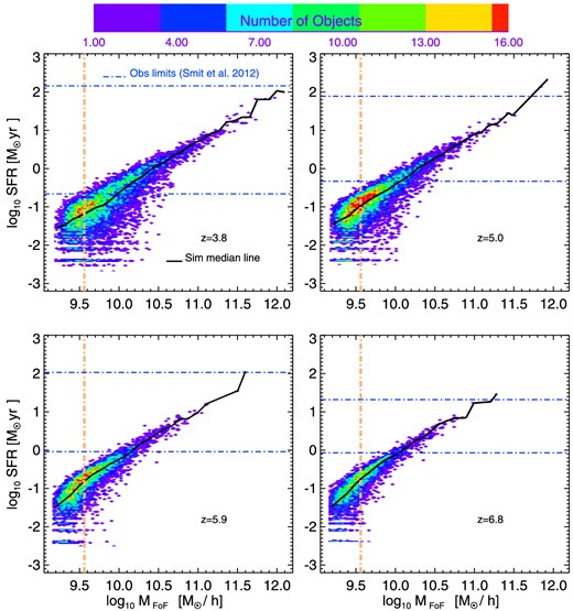
Density plots of the SFR–total halo mass relation for the Kr24_eA_sW run at redshifts z ∼ 4–7. The blue dot–dashed horizontal lines represent the observational limits in the range of SFR of Smit et al. (2012). The orange dot–dashed vertical line is our mass confidence limit (see Section 3.1). The black solid line is the median line through the points of the density plots.
The relation between SFR and total halo mass is not observable, but we explore it to evaluate the effects of different feedback mechanisms and IMFs, and the impact of metal cooling in our simulations. In Fig. 2, we compare the median lines of the SFR(MFoF) density plots for all the runs with box size L = 24 Mpc h−1. At each redshift, a panel showing ratios between the different simulations and the Kr24_eA_sW run (black solid line) is included. At redshift z = 6.8, we see that different configurations are not distinct, except for the no-feedback (Ch24_NF – magenta triple dot–dashed line) and the momentum-driven wind (Ch24_eA_MDW – dark green dashed line) cases. By comparing the Ch24_NF run with all the other simulations, we can see that feedback is already in place at z ∼ 7 and lowers the SFR at any given halo mass. Momentum-driven winds effectively quench the SFR in low-mass haloes, but are less efficient than constant winds (with fixed velocity and mass loading factor η = 2) in high-mass haloes (MFoF ≳ 1010.5 M⊙ h−1, for the velocity normalization that we use). This is due to the fact that in this case η scales with the inverse of the wind velocity (|$\eta \propto v_{\rm w}^{-1}$|, see Section 2.1). The same trends are visible at redshifts z = 5.9 and z = 5.0, with the differing behaviour of the Ch24_NF and Ch24_eA_MDW runs more marked at lower redshift.
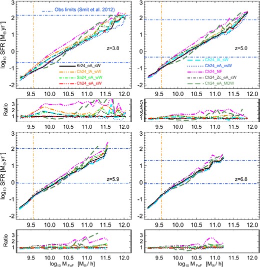
SFR–total halo mass relation (median lines through density plots) for all the runs of Table 1 with box size equal to 24 Mpc h−1. The blue dot–dashed horizontal lines represent the observational limits in the range of SFR of Smit et al. (2012). The orange dot–dashed vertical line is our mass confidence limit (see Section 3.1). At each redshift, a panel showing ratios between the different simulations and the Kr24_eA_sW run (black solid line) is included.
Finally, at redshift z = 3.8, different feedback configurations show different behaviour. The effect of SN-driven winds is important for all haloes: from the least to the most massive. In the less massive haloes (MFoF ≲ 1011 M⊙ h−1), both strong and weak winds remove gas from the central regions and prevent the formation of new stars. On the other hand, in the most massive haloes weaker winds are not able to efficiently expel gas from the high-density regions and quench the star formation.
In Fig. 3, we highlight the effect of different forms of feedback, metal cooling and IMF on the SFR(MFoF) relation at z = 3.8. To explore the impact of galactic winds, in the top left panel, we compare the Ch24_eA_sW (red triple dot–dashed line) and the Ch24_eA_vsW (blue dotted line) runs. These runs have exactly the same configuration with the exception of velocity of the winds (450 km s−1 and 550 km s−1, respectively). As argued above, at high masses (M ≳ 1011 M⊙ h−1), the SFR is lower when the wind velocity is higher (i.e. the blue dotted line is always below the red triple dot–dashed line).
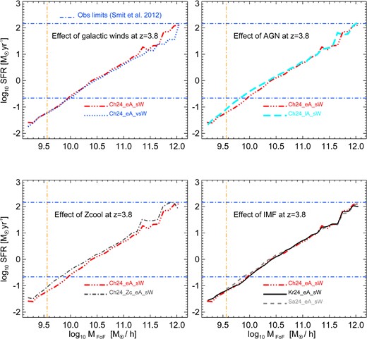
SFR–total halo mass relation (median lines through density plots) at z = 3.8. We evaluate the effects of galactic winds (top left panel), AGN feedback (top right panel), metal cooling (bottom left panel) and choice of IMF (bottom right panel). The blue dot–dashed horizontal lines represent the observational limits in the range of SFR of Smit et al. (2012). The orange dot–dashed vertical line is our mass confidence limit (see Section 3.1).
On the other hand, the effect of AGN feedback is particularly visible at low masses (M ≲ 1010.5 M⊙ h−1). This can be seen by comparing the values of the SFR(M) relation for the Ch24_eA_sW (red triple dot–dashed line) and the Ch24_lA_sW (cyan dashed line) runs (top right panel of Fig. 3). These runs have the same wind strength, but different AGN configurations. In the first case, we adopted the ‘early AGN’ scheme, where we reduced the halo mass and the star mass fraction thresholds (Mth and f⋆) to seed a central SMBH of mass Mseed, with respect to the ‘late AGN’ scheme. However, the radiative efficiency (ϵr) and the feedback efficiency (ϵf) are the same in the two regimes (see Section 2.1). Tescari et al. (2014) discussed how decreasing the threshold mass for seeding an SMBH increases the effect of AGN feedback on haloes with low masses/SFRs, since we impose high black hole/halo mass ratios in small galaxies at early times. As a result, at low masses SFR lA(MFoF) > SFR eA(MFoF), where the subscripts refer to late and early AGN feedback, respectively. At the same time, the effect of AGN feedback on the most massive haloes is minimal, since in these objects the central SMBH has not yet reached the self-regulation regime, where a lot of energy is released and further star formation prevented.
By comparing the Ch24_Zc_eA_sW run (dark grey dot–dashed line) with the Ch24_eA_sW run (red triple dot–dashed line) in Fig. 2, we are able to test how metal cooling affects the SFR–MFoF relation. We see that at all redshifts considered, the SFR at a given halo mass is always higher in the case of the simulation that includes metal cooling. This is due to the fact that when metals are taken into account in the cooling function, the enriched gas inside haloes can cool more efficiently and produce more stars than the same amount of gas of pristine composition. The bottom left panel of Fig. 3 shows the comparison between the SFR(MFoF) relations of Ch24_Zc_eA_sW and Ch24_eA_sW runs at redshift z = 3.8.
Since the total integrated amount of gas converted into ‘stars’ is the same for different IMFs, for our simulations, the choice of IMF plays a minor role (Tescari et al. 2014). In fact, the run with a Kroupa IMF (Kr24_eA_sW — black solid line) and the simulation with Chabrier IMF (Ch24_eA_sW – red triple dot–dashed line) have almost the same SFR(MFoF) relation at all halo masses and redshifts.
In the bottom right panel of Fig. 3, we clarify this by showing, in addition to the previous two runs, the SFR(MFoF) relation at z = 3.8 for a simulation with early AGN, strong winds and Salpeter (1955) IMF: (Sa24_eA_sW − dashed grey line).5 We are comparing models that do not include metal cooling, therefore the source of any difference between these simulations is the number of stars above the SNII mass threshold.
To conclude, we note that at all redshifts considered, when the mass confidence limit is approached (orange dot–dashed vertical lines in Figs 2 and 3), all the simulations show exactly the same trend because the different feedback configurations start to be numerically poorly resolved. However, we stress that this always happens outside the observational window of Smit et al. (2012), which we adopted to perform our analysis. In Appendix A, we present the resolution and box size tests using simulations with L = 18 Mpc h−1 and L = 12 Mpc h−1. These tests show that different configurations are convergent to ∼0.1 dex inside the observational limits, with the caveat that simulations with smaller box size are dominated by poor statistics in the high-mass end of the SFR–MFoF relation.
3.2 The observed star formation rate–stellar mass relation
In this section, we discuss the observed SFR–stellar mass relation (SFR–M⋆). We use three sets of observations.
The observed galaxy star formation rate–stellar mass relation at z ∼ 4–7 from Drory & Alvarez (2008, observed frame I-band selected sample – green dashed + dotted lines), Bouwens et al. (2012, drop-outs selection – blue triple dot–dashed lines + light blue shaded regions) and de Barros, Schaerer & Stark (2014, drop-outs selection – dark green filled squares – No Nebular emission + red filled circles – Nebular emission). The open symbols are the median values of de Barros et al. (2014) that according to the authors suffer from low statistics. The numbers represent the number of galaxies that were used to obtain the median SFR at a given M⋆. The light blue shaded regions represent the statistical error of the SFR–M⋆ relation from Bouwens et al. (2012), estimated by varying the normalization factor in equation (6). The green dotted lines represent the 0.3 dex scatter of the SFR–M⋆ relation from Drory & Alvarez (2008).
We stress that, according to Bouwens et al. (2012) dust corrections increase the normalization of the SFR(M⋆) relation by more than a factor of 2. This implies that a dwarf galaxy with almost no dust, and stellar mass log (M⋆/M⊙) ≃ 8.5 at z ∼ 4, should have an SFR ∼1.9 times higher if dust corrections are applied.8 However, Stark et al. (2009) pointed out that the inclusion of dust corrections should not lead to an increase in the normalization over time. This could mean that the dust corrections of Bouwens et al. (2012) at a fixed stellar mass are overestimated.
The second set of observations we consider comes from de Barros et al. (2014). Galaxies at z ∼ 3, 4, 5 and 6 were selected via the presence of the Lyman-break as it is redshifted through the U, B, V, and i bands, respectively. The authors state that their colour criteria are very similar to Bouwens et al. (2012). de Barros et al. (2014) investigated the effect of different choices of the SFH (constant, decreasing and rising) and nebular emission lines. Stellar masses and SFRs were obtained using spectral energy distribution (SED) fitting taking into account attenuation from intergalactic and interstellar media. For consistency, we consider the constant SFH model since Bouwens et al. (2012) assumed the same. We plot the results of de Barros et al. (2014) in Fig. 4 (dark green squares). We can see that the inclusion of nebular emission to this model is responsible for a very small shift of the results to smaller masses (red circles of Fig. 4). The results of the authors can be found in table A1 of their work. According to de Barros et al. (2014), there is a very small number of objects in the brightest and faintest bins at each redshift. Therefore, they state that it is considered more appropriate to take into account only the three intermediate bins to examine trends of the physical properties.

Fig. 4 illustrates the range of SFR–M⋆ relations derived using different sample selections and dust corrections. We can see that the analysis of Drory & Alvarez (2008) is able to probe galaxies with higher masses due to their selection criteria. The sample of these authors includes high mass and obscured galaxies10 that are not found by the drop-outs selection of Bouwens et al. (2012) and de Barros et al. (2014). The drop-out selection can affect the obtained SFR–M⋆ relation since it takes into account only actively star-forming galaxies. Karim et al. (2011) used 1.4 GHz luminosities and SED fitting to estimate the SFR–M⋆ relation at z ∼ 0.2–3.0 for a mass selected sample. When the authors include only star-forming galaxies in their analysis, the average SFR at a fixed mass is larger, especially at the high-mass end of the distribution where quiescent galaxies are present. This effect tends to increase the values of SFR at a fixed mass for the relations obtained by Bouwens et al. (2012) and de Barros et al. (2014).
de Barros et al. (2014) state that their stellar mass–luminosity relation is consistent with the one found by González et al. (2011). However, the SFR–M⋆ relations of Fig. 4 are quite different. The above studies have similar selection criteria and assume almost the same stellar mass–luminosity relation. However, they retrieve SFRs with different methods. To estimate the SFR at a fixed mass, Bouwens et al. (2012) used corrections based on UV-continuum slopes (Meurer et al. 1999) and the Kennicutt (1998) relation, while de Barros et al. (2014) based their results on SED fitting. We see that the SFRs at a fixed mass are higher in the case of Bouwens et al. (2012). The results of de Barros et al. (2014) and Drory & Alvarez (2008) for the SFR–M⋆ are in good agreement with each other. Both surveys utilized SED fitting for their analysis. Bauer et al. (2011) investigated how different methods for the determination of the intrinsic SFR can affect the observed SFR–M⋆ relation. The authors concluded that the best way to determine the amount of dust extinction and the intrinsic SFR is using multiwavelength SED fitting.
Another difference between the relations shown in Fig. 4, is that Drory & Alvarez (2008) calculated the average SFR–M⋆ relation, while Bouwens et al. (2012) used the median M⋆/L ratios from González et al. (2011). Different results are expected using average rather than median M⋆/L ratios, since using average ratios would increase the masses. The reason is that in the case of medians, calculations will not take into account the large amounts of stellar mass that reside in the high M⋆ tail of the mass distribution.
In conclusion, there is a tension between the SFR–M⋆ relations reported in the literature at z ∼ 4–7. The main reason for this is that observers use different methods and techniques to obtain the intrinsic SFRs and dust corrections. In addition, selection effects can play an important role for the determination of the slope. For instance, Lyman-break selection is biased to detect the most star-forming systems at a fixed stellar mass. This effect is more severe for the low-mass end (Reddy et al. 2012) and high-mass end of the distribution (Heinis et al. 2014). This bias increases the normalization of the retrieved SFR–M⋆ relation and possibly makes its slope artificially shallower.
3.3 Comparison between simulated and observed SFR–M⋆ relation
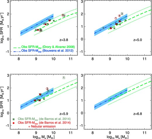
In this section, we compare the observed and simulated SFR–M⋆ relations at high redshift. The evolution of this relation is important since it provides key constraints on the stellar mass assembly histories of galaxies, and also the determination of the GSMF. In Fig. 6, we present a density plot of our fiducial run Kr24_eA_sW at redshifts z ∼ 4–7. In each panel, the red triple dot–dashed line is a least-square linear fit in log–log space to all the points, and the black solid line their median value in mass bins of 0.1 dex. The halo mass confidence limit of 100 DM particles discussed in Section 3.1 corresponds to a stellar mass limit of M⋆ ∼ 107.5 M⊙. However, in our analysis we take into account objects with M⋆ ≥ 107.75 M⊙, which is roughly the mass limit of the current observations (González et al. 2011). Overplotted are the observed galaxy SFR(M⋆) relations from Drory & Alvarez (2008, observed frame I-band selected sample – green dashed + dotted lines), Bouwens et al. (2012, drop-outs selection – blue triple dot–dashed lines + light blue shaded regions) and de Barros et al. (2014, drop-outs selection – dark green filled squares – No Nebular emission + red filled circles – Nebular emission). We find that the simulated relation does not follow either of the three observed relations (and the difference increases at lower redshift where the scatter in the simulated data also increases). In particular, the observed relations are heavily weighted towards high masses, while the opposite is true for the simulated relation. We see that the SFR–M⋆ relations obtained from our cosmological hydrodynamic simulations (red triple dot–dashed lines, Fig. 6) have a lower normalization than all the observed relations. This could be due to the fact that observations are unable to detect the faintest and less star-forming objects at a fixed stellar mass.11 For this reason, the observed SFR(M⋆) end up having artificially higher normalization. This bias effect is exacerbated in the low stellar mass tail of the distribution (see e.g. fig. 26 of Reddy et al. 2012, and related discussion). Moreover, the intrinsic (bias corrected) observed relation has a slope close to unity, which is in good agreement with cosmological hydrodynamic simulations. In the next paragraphs of this section, we discuss in detail the implications of observational biases and different feedback prescriptions on the SFR–M⋆ relation.
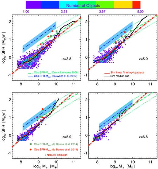
Density plots of the SFR–stellar mass relation for our fiducial run Kr24_eA_sW at redshifts z ∼ 4–7. In each panel, the black solid line is the median line through the density plot, while the red triple dot–dashed line is the linear fit (in log–log space, calculated using a least-square fit) to the points of the density plot. Overplotted are the observed galaxy SFR(M⋆) relations from Drory & Alvarez (2008, observed frame I-band selected sample – green dashed + dotted lines), Bouwens et al. (2012, drop-outs selection – blue triple dot–dashed lines + light blue shaded regions) and de Barros et al. (2014, drop-outs selection – dark green filled squares – No Nebular emission + red filled circles – Nebular emission). The light blue shaded regions represent the statistical error of the SFR–M⋆ relation from Bouwens et al. (2012), estimated by varying the normalization factor in equation (6). The green dotted lines represent the 0.3 dex scatter of the SFR–M⋆ relation from Drory & Alvarez (2008).
In Fig. 7, we compare the median lines of the SFR–stellar mass density plots for all the runs of Table 1 with box size L = 24 Mpc h−1. In Appendix A, we will also show the resolution and box size tests using simulations with L = 18 Mpc h−1 and L = 12 Mpc h−1. These tests demonstrate that the SFR–M⋆ relation converges at all redshifts considered. At redshift z = 6.8, the different configurations are not distinct (bottom right panel). The same is true at z = 5.9 (bottom left panel), except in the case of the Ch24_NF (magenta triple-dot dashed line), where the absence of feedback leads to slightly higher SFRs at fixed stellar masses. The presence of feedback lowers the SFR at a given M⋆ at redshifts z = 5 and z = 3.8 (top right and left panels, respectively). In our simulations, the feedback prescription, choice of IMF and metal cooling all seem to play a small role in the normalization and slope of the simulated SFR–M⋆ relation. Lastly, the momentum-driven winds run is in good agreement with all the constant wind models and the observations.
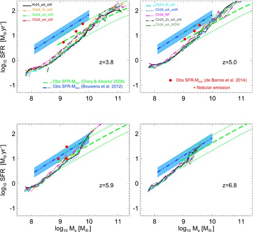
Median lines of the star formation rate–stellar mass density plots for all the runs of Table 1 with box size equal to 24 Mpc h−1. Overplotted are the observed galaxy SFR(M⋆) relations from Drory & Alvarez (2008, observed frame I-band selected sample – green dashed + dotted lines), Bouwens et al. (2012, droup-outs selection – blue triple dot–dashed lines + light blue shaded regions) and de Barros et al. (2014, droup-outs selection – nebular emission – red filled circles). Line-styles of different simulations are as in Fig. 2.
Star formation is thought to be regulated by the balance between the rate at which the cold gas that creates stars is accreted on to the galaxy, and feedback responsible for quenching the SFR (Finlator & Davé 2008; Bouché et al. 2010; Dutton et al. 2010). Generally, a linear SFR–M⋆ relation is expected from cosmological hydrodynamic simulations (Birnboim & Dekel 2003; Davé 2008; Finlator, Oppenheimer & Davé 2011a). This implies a star-forming scenario in which the galaxies build up mass exponentially with time (Stark et al. 2009; Lee et al. 2011; Papovich et al. 2011). It is thought that feedback may affect the slope of the SFR(M⋆) relation, but a slope near unity is a generic result of numerical models owing to the dominance of cold mode accretion, which produces rapid, smooth infall (Davé 2008). Moreover, according to Schaye et al. (2010), this is also related to the fact that galaxies form stars in a self-regulated fashion. To interpret the SFR(M⋆) relation, it is therefore important to note that M⋆ and SFR are both correlated with feedback and cooling. For example, the presence of strong SN feedback lowers the SFR for a galaxy and at the same time lowers its stellar mass with respect to the no feedback run. For this reason, the differences between different feedback configurations are very small for these redshifts. However, a larger discrepancy between SFR–M⋆ relations simulated with different feedback prescriptions is expected for lower redshifts (Haas et al. 2013a,b).
The intrinsic SFR(M⋆) relations in our fiducial simulation Kr24_eA_sW (see the red triple dot–dashed lines in Fig. 6) are as follows:
z ∼ 4: SFR ≃ (2.0 M⊙ yr−1) × (M⋆/109 M⊙)0.81,
z ∼ 5: SFR ≃ (3.2 M⊙ yr−1) × (M⋆/109 M⊙)0.80,
z ∼ 6: SFR |$\simeq \left(4.7\,{\rm M_{\rm {\odot }}\,yr^{-1}}\right)\times \left({M_{\star }/10^{9}\,\mathrm{M}_{{\odot }}}\right)^{0.88}$|,
z ∼ 7: SFR |$\simeq \left(5.9\,{\rm M_{\rm {\odot }}\,yr^{-1}}\right)\times \left({M_{\star }/10^{9}\,\mathrm{M}_{{\odot }}}\right)^{0.90}$|.
We find that the normalization factor evolves from z = 7 to 4, while the exponent is nearly constant with an averaged value of ∼0.85. The predicted relation from simulations has a slope almost ∼1, regardless of the configuration used. Wilkins et al. (2013) also find in their simulations that the intrinsic M⋆/LUV–LUV relation is almost flat, implying a linear SFR–M⋆ relation. Furthermore, Finlator et al. (2011a) found an almost linear relation between star formation and stellar mass. For comparison, Bouwens et al. (2012) estimated the dust-corrected SFR(M⋆) relation and found that SFR |$\propto {M}_{\star }^{0.73}$| (while the relation without including dust attenuation was found to be SFR |$\propto {M}_{\star }^{0.59}$|). Thus, dust attenuation plays an important role in the exponent of the SFR–M⋆ relation.
As discussed above, our simulations predict lower values of SFR than observations, especially for objects with small stellar masses. The large difference between observed and predicted SFRs from cosmological hydrodynamic simulations in the literature indicates either that the simulations provide an incomplete picture of galaxy assembly and cold accretion, or that the observational results are biased. Reddy et al. (2012) discussed the implications of various sample biases in the observed SFR-M⋆ relation. The authors determined both SFR and stellar mass for intermediate redshift galaxies (1.4 < z < 2.7) by means of an SED fitting procedure. Using mock samples, SFR and M⋆ were found to be positively correlated with an intrinsic slope of ∼1. However, a linear least-squares fit directly to the observational data, showed a shallower slope of ∼0.30. This bias is due to the fact that their observational sample was selected based on UV luminosities (and not stellar masses). As a consequence, galaxies with larger SFRs at a given stellar mass were preferentially selected. According to Reddy et al. (2012), the SFR at log (M⋆/M⊙) = 9.25 is artificially ∼3–4 times larger than the intrinsic value due to this observational selection bias. Bouwens et al. (2012) stressed that their analysis is representative of a luminosity-selected sample and that this bias can affect their results. We see that our simulations predict lower values of SFR at a fixed mass than Bouwens et al. (2012), especially for low-mass objects. We are in better agreement with the results of de Barros et al. (2014). These authors compiled their sample using the same selection criteria as Bouwens et al. (2012), but computed SFRs and stellar masses using the more reliable SED-fitting technique.
On the other hand, the I-band selected sample of Drory & Alvarez (2008) allows them to include galaxies with larger masses and the selection of stellar mass in obscured objects. However, their magnitude cut results in a sample which is incomplete for objects with low stellar masses/SFRs. From Fig. 7, we see that our simulations are in good agreement with their proposed SFR(M⋆) relation. We checked that there is also a good consistency between our simulations and the recent results of Salmon et al. (2014). Despite the good consistency between our numerical results and these observations, the simulated relations tend to be steeper.
It is worth mentioning that, although not presented in this paper, the SFR–M⋆ relation proposed by Stark et al. (2009, rest-frame UV-selected sample of galaxies without dust corrections) is in almost perfect agreement with our results. The authors stressed that dust corrections could introduce considerable errors into the observed relation, so they limited their analysis to the relationship between stellar mass and emerging luminosity (i.e. the luminosity inferred from the flux that escapes the galaxy without applying any dust corrections). According to Stark et al. (2009), the dust correction law given by Meurer et al. (1999) adds a significant random scatter to the observed relation, and possibly cancels any existing trend with luminosity and redshift.12 Their results also suggest that dust corrections could have a small impact on the intrinsic SFR at a fixed stellar mass for z ∼ 4–7.
In conclusion, we find that at stellar masses M⋆ ≲ 109 M⊙ both observations and simulations contain uncertainties, with observations being incomplete and simulations lacking in resolution. For masses M⋆ ≳ 109 M⊙, our simulations are in agreement with the observations of Drory & Alvarez (2008) and Salmon et al. (2014). In addition, there is a good consistency between our results and the observations of de Barros et al. (2014), who used SED fitting to obtain the intrinsic SFRs and stellar masses in their Lyman-break selected sample. Note that these authors were only able to probe a small mass interval (log (M⋆/M⊙) ∼ 9.1 − 9.7 at z ∼ 4). Specifically, they do not take into account objects in the low- and high-mass ends of the distribution, where Lyman-break observations are potentially more affected by selection effects. On the other hand, there is disagreement between our simulations and the observations of Bouwens et al. (2012) (especially at z = 3.8). Our results suggest that their Lyman-break selection may miss a significant number of galaxies, especially at low masses (Bouwens et al. 2012; Reddy et al. 2012; Heinis et al. 2014). This conclusion is also supported by the recent work of Wyithe, Loeb & Oesch (2013). In the next section, we show that this incompleteness leads to large uncertainties in the determination of the GSMF.
Finally, our simulations predict a tight SFR–M⋆ relation which is broadly consistent with the results of Whitaker et al. (2012), who found the scatter of the intrinsic relation to be ∼ 0.17.
4 THE GALAXY STELLAR MASS FUNCTION
4.1 Observational GSMF
In this section, we compare our simulations with the observed GSMFs from Marchesini et al. (2009), González et al. (2011), Lee et al. (2012) and Santini et al. (2012). Marchesini et al. (2009) and Santini et al. (2012) used K-selected galaxy samples and were able to determine the mass function for the most massive galaxies within the redshift range we study. Selecting galaxies from a K-selected sample includes all galaxies rather than only those that are active and brightly star-forming (as in a Lyman-break selected sample). However, even the lowest mass galaxies selected by these studies are among the most massive galaxies known at z > 3 and provide information only about the high end of the GSMF. In addition, these massive galaxies are strongly clustered, which could lead to biased estimations due to the effect of cosmic variance. González et al. (2011) and Lee et al. (2012) presented GSMFs based on rest-frame UV-selected samples, enabling selection of less massive objects. However, the relationships they retrieved are valid only for star-forming galaxies. In general, the various GSMFs presented in the literature are in good agreement at z ≲ 3.5, but differences between studies exist at higher redshift (z ≳ 4). In the following, we describe each measurement and compare the different observational results. The cosmology assumed is the same in all cases (H0 = 70 km s−1 Mpc−1) except for Lee et al. (2012) (H0 = 72 km s−1 Mpc−1). Since most of the authors assumed a Salpeter (1955) IMF, we corrected observed GSMFs to a Salpeter IMF whenever the original choice was different.
Marchesini et al. (2009) measured GSMFs of galaxies at redshifts 1.3 < z < 4.0. The authors used the combined optical and IR data from three different surveys (NIR MUSYC, ultradeep FIRES and GOODS-CDFS), providing a large area of the sky, so that errors due to cosmic variance should be reduced. In the top left panel of Fig. 8, the green filled circles with error bars show the GSMF of Marchesini et al. (2009) at z ∼ 4. We multiplied the stellar masses of Marchesini et al. (2009) by 1.6 since the authors used a pseudo-Kroupa IMF instead of a Salpeter (1955) IMF.13

Santini et al. (2012) estimated GSMFs in six different redshift intervals between z ∼ 0.6 and z ∼ 4.5 using Early Release Science (ERS) observations taken with the WFC3 in the GOODS-S field. Thanks to deep near-IR observations, they were able to sample the GSMF at masses lower than previous IR studies. However, the authors stated that despite the good agreement with previous work, the limited area of their survey could affect the results at the highest masses (due to cosmic variance). We present the analytic result of Santini et al. (2012) in the top left panel of Fig. 8 (magenta dashed line).
On the other hand, González et al. (2011) estimated the GSMF at a given redshift by combining the rest-frame UV luminosity function (LF) with the LUV–M⋆ relation measured at z ∼ 4. They used the z ∼ 4–7 UV-LFs from Bouwens et al. (2007, 2011, Hubble-WFC3/IR camera observations of the ERS field combined with the deep GOODS-S Spitzer/IRAC data). As a result, the incompleteness-corrected MFs derived by González et al. (2011) are substantially steeper at low masses than previously found at these redshifts (where incompleteness corrections were not taken into account). The González et al. (2011) results are shown as the blue filled squares with error bars in Fig. 8.
Lee et al. (2012) investigated how star-forming galaxies typically assemble their mass between redshifts z ∼ 4 and z ∼ 5. We present the fit to the GSMFs for star-forming galaxies found in Lee et al. (2012) in the top panels of Fig. 8 (orange dashed lines). Since the authors assumed a Chabrier (2003) IMF, we convert their results to a Salpeter (1955) IMF by adding 0.16 dex to stellar masses. As noted, the observations from González et al. (2011) and Lee et al. (2012) (i.e. the UV-selected surveys) do not represent the total SMF of all galaxies at a given redshift, rather they provide information about how much of the cosmic stellar mass density is distributed in actively star-forming and UV-bright galaxies.
The K-selected GSMFs from Santini et al. (2012) and Marchesini et al. (2009) are in agreement at redshift z ∼ 4. Similarly, González et al. (2011) is in agreement with Lee et al. (2012) at z ∼ 4, in the mass bin 108.5 M⊙ ≲ M⋆ ≲ 109.5 M⊙. At z ∼ 5, the overall normalization of the González et al. (2011) GSMF is 50 per cent higher than in Lee et al. (2012).14 However, where results can be directly compared at z ∼ 4, there is an offset in amplitude between Lyman-break and K-selected GSMFs.
4.2 Comparison between simulated and observed galaxy stellar mass functions
We next compare the GSMFs obtained from our simulations with the observed GSMFs discussed in the previous section. Simulations of the GSMF with box size L = 24 Mpc h−1 are shown in Fig. 9.15 At each redshift, a panel showing ratios between the different simulations and the Kr24_eA_sW run (black solid line) is included. At z = 6.8 and z = 5.9, our results are in agreement with the results from González et al. (2011), while at lower redshifts our simulations overpredict the number of star-forming selected galaxies of all stellar masses with respect to their observations.16 In addition, at z < 5, our simulated GSMFs are consistent with the K-selected GSMFs of Marchesini et al. (2009) and Santini et al. (2012). Below we discuss the results at each redshift in more detail.
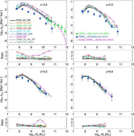
Galaxy stellar mass functions for all the runs of Table 1 with box size equal to 24 Mpc h−1. Overplotted are the observational results of Marchesini et al. (2009, green filled circles with error bars), González et al. (2011, blue filled squares with error bars) and Santini et al. (2012, magenta dashed line). At each redshift, a panel showing ratios between the different simulations and the Kr24_eA_sW run (black solid line) is included. Line-styles of different simulations are as in Figs 2 and 7.
At redshift z = 6.8 (bottom right panel of Fig. 9), all simulations show the same trend, regardless the configuration used (strength of feedback, inclusion of metal cooling and choice of IMF). Only the no feedback (Ch24_NF) and the very strong winds (Ch24_eA_vsW) cases show a small variation with respect to the other runs. This dependence is consistent with the results of Tescari et al. (2014) for the SFRF.
At z = 5.9 (bottom left panel), all simulations are also in good agreement with observations (apart from the no feedback run). In the no feedback case, we have an overproduction of systems in the high-mass tail of the distribution (log (M⋆/M⊙) ≳ 9.3) with respect to all the other simulations, due to the overcooling of gas.
At z = 5.0 (top right panel), all configurations predict more galaxies than observed in almost the whole stellar mass range. Note that the GSMF of the fiducial Kr24_eA_sW run (black solid line) is truncated at log (M⋆/M⊙) ∼ 9.8. This is due to low number statistics at higher masses. Therefore, in order to have a fair comparison with all the other simulations, we decided to exclude this region of the Kr24 GSMF.
The behaviour of different simulations only becomes clear at z = 3.8 (top left panel). The no feedback case is ruled out by observations of galaxies based on both Lyman-break and K-band selection. In the following sub-sections and in Fig. 10, we highlight the impact of SN-driven galactic winds, AGN feedback, metal cooling and momentum-driven winds on the GSMF at z = 3.8.
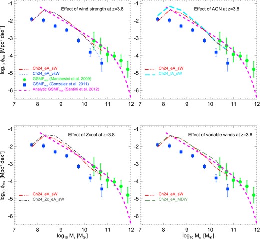
Galaxy stellar mass functions at z = 3.8. We evaluate the effects of galactic wind strength (top left panel), AGN feedback (top right panel), metal cooling (bottom left panel) and momentum-driven winds (bottom right panel) on the GSMF. Overplotted are the observational results of Marchesini et al. (2009, green filled circles with error bars), González et al. (2011, blue filled squares with error bars) and Santini et al. (2012, magenta dashed line).
4.2.1 Effect of SN and AGN feedback
We start by analysing simulations which have a Chabrier IMF, energy-driven galactic winds and no metal cooling: Ch24_lA_wW, Ch24_lA_sW, Ch24_eA_sW and Ch24_eA_vsW. In the most massive galaxies (log (M⋆/M⊙) ≳ 9.8), the run with late AGN feedback and weak winds (Ch24_lA_wW) produces the highest values of the GSMF. The runs Ch24_lA_sW and Ch24_eA_sW have strong winds with late and early AGN feedback, respectively. These two simulations do not show any difference at high stellar masses. However, the resulting GSMFs are lower than the Ch24_lA_wW run. Finally, the very strong winds case (Ch24_eA_vsW) has the lowest value of the GSMF in the high-mass tail. We highlight the effect of SN feedback in the top left panel of Fig. 10, by comparing results from the Ch24_eA_sW and Ch24_eA_vsW runs.
The situation is different at low stellar masses (log (M⋆/M⊙) ≲ 9.0). In this range, the Ch24_lA_wW run produces more systems with respect to the other three simulations. However, the Ch24_lA_sW and Ch24_eA_sW runs are not equal at these low masses. The GSMF of Ch24_eA_sW is lowered by ∼0.2 dex. This enhanced effect of AGN feedback, labelled in the low-mass end is related to our black hole seeding scheme (see below). The top right panel of Fig. 10 shows the effect of AGN feedback by comparing the Ch24_lA_sW run and the Ch24_eA_sW run.
In Tescari et al. (2014) and in Section 3.1, we discussed the interplay between SN-driven galactic winds and AGN feedback in our simulations. Galactic winds start to be effective before AGN and therefore shape the whole GSMF. In low-mass haloes, the effect of weak and strong winds is the same: both configurations efficiently quench the ongoing star formation by removing gas from the high-density central regions. In high-mass haloes, weaker winds become less effective. As a result, the GSMF for Ch24_eA_vsW is lower than the GSMF for Ch24_eA_sW (top left panel of Fig. 10).
We use two configurations for the AGN feedback, labelled ‘early’ and ‘late’. In our model, we seed all the haloes above a given mass threshold with a central SMBH. In the ‘early AGN’ configuration, we reduced this threshold and therefore increased the effect of AGN feedback on haloes with low mass by construction. For this reason, the GSMF for Ch24_eA_sW is lower than the GSMF for Ch24_lA_sW in the low end of the distribution, log (M⋆/M⊙) ≲ 9.0 (see the top right panel of Fig. 10). At high masses, SMBHs have not yet reached a regime of self-regulated growth and therefore do not significantly affect the GSMF. In fact, the GSMF for Ch24_eA_sW is equal to the GSMF for Ch24_lA_sW for log (M⋆/M⊙) ≳ 9.5. We stress that the radiative efficiency (ϵr) and the feedback efficiency (ϵf) are each the same in the two AGN configurations.
4.2.2 Effect of metal cooling
The simulation with metal cooling (Ch24_Zc_eA_sW), shows an increase of the GSMF at all masses with respect to the corresponding simulation without metal cooling (Ch24_eA_sW). This is due to the fact that when metals are included in the cooling function, the gas can cool more efficiently and produce more stars than gas of primordial composition. The effect of metal cooling is visible in the bottom left panel of Fig. 10.
4.2.3 Effect of IMF
The choice of IMF plays a minor role in the simulated GSMFs. By comparing the Kr24_eA_sW run (Kroupa IMF) with the Ch24_eA_sW run (Chabrier IMF), we see that the only small difference is at redshift z = 3.8, where the run with Chabrier IMF results in slightly less galaxies with M⋆ ≳ 1010 M⊙ (top left panel of Fig. 9).
4.2.4 Constant- versus momentum-driven galactic winds
The physics of the SNe feedback remains an uncertainty in galaxy formation modelling (Springel & Hernquist 2003; Oppenheimer & Davé 2006; Tescari et al. 2009; Choi & Nagamine 2011; Tescari et al. 2011; Puchwein & Springel 2013), and we have computed results using two different galactic winds schemes. In Fig. 9, we compare the evolution of the GSMF for the Ch24_eA_sW run (Chabrier IMF, early AGN feedback and energy-driven galactic winds of constant velocity vw = 450 km s−1 – red triple dot–dashed line) and the Ch24_eA_MDW run (Chabrier IMF, early AGN feedback and momentum-driven galactic winds – dark green dashed line).
At redshift z = 6.8, 5.9 and 5.0, we find that the two simulations are in excellent agreement. At z = 3.8, the only notable difference is a slight overproduction of systems with stellar masses log (M⋆/M⊙) ≳ 9.5 for the Ch24_eA_MDW run (bottom right panel of Fig. 10). This is due to the fact that momentum-driven winds are less efficient than constant winds in the most massive haloes. As we showed in Tescari et al. (2014), at z ≳ 4 the effect of the two different galactic wind implementations on the SFRF is significant, while the two schemes result in almost the same GSMF evolution.
5 BEST MODEL AND DISCUSSION
In Fig. 11, we show the GSMFs at redshifts z ∼ 4–7 for our fiducial model Kr24_eA_sW with Kroupa IMF, early AGN feedback and strong energy-driven galactic winds of constant velocity vw = 450 km s−1 (black solid lines). We include the Poissonian uncertainties for the simulated GSMFs (black error bars), in order to provide an estimate of the errors from our finite box size. In this figure, we also compare this fiducial model with the observations discussed in Section 4.1.
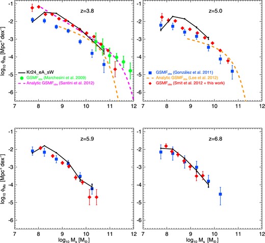
Galaxy stellar mass functions at z ∼ 4–7 for our fiducial model with Kroupa IMF, early AGN feedback, constant galactic winds (vw = 450 km s−1) and box size equal to 24 Mpc h−1 (black solid lines). The black error bars are the Poissonian uncertainties of the simulated GSMFs. Overplotted are the observational results of Marchesini et al. (2009, green filled circles with error bars), González et al. (2011, blue filled squares with error bars), Lee et al. (2012, orange dashed lines) and Santini et al. (2012, magenta dashed line). At each redshift, the red diamonds with error bars show the GSMF recovered by combing the stepwise determination of the star formation rate function from Smit et al. (2012) with our simulated intrinsic SFR–M⋆ relation (see Section 5).
While at z > 5, our simulated GSMFs are in good agreement with the results inferred by González et al. (2011); at 3.8 ≤ z ≤ 5, there is disagreement between their Lyman-break selected GSMF and our numerical results. Our runs predict ∼3 times more objects than those found by González et al. (2011). However, at redshift z ∼ 4, we are in excellent agreement with the results of Marchesini et al. (2009), Santini et al. (2012) (the K-selected samples) and the new data of Duncan et al. (2014). Santini et al. (2012) compared their results with the semi-analytic models of Menci et al. (2006), Monaco, Fontanot & Taffoni (2007), Wang et al. (2008) and Somerville et al. (2012), at the same redshift. These semi-analytic models are also broadly consistent with observations, even though they all underestimate the stellar mass function at the high-mass end.
Jaacks et al. (2012) and Wilkins et al. (2013) have previously used cosmological hydrodynamic simulations to model the results of González et al. (2011). Both studies also found disagreement with these observations. In particular, Wilkins et al. (2013) claimed that the tension between simulated and observed GSMFs arises for two reasons. First, at z ∼ 5, there is a difference in the slope of the UV LF at low LUV. According to the authors, this difference is probably due to the fact that feedback in their simulations is not efficient enough for galaxies with M⋆ < 109 M⊙ h−1. The second reason is that González et al. (2011) did not take into account the evolution in the assumed LUV–M⋆ relation. As described in Section 4.1, at 4 ≤ z ≤ 7, the authors used the LUV–M⋆ relation calibrated at redshift z ∼ 4. However, Wilkins et al. (2013) found in their simulations that this relation evolves significantly over time and this is partly responsible for the inconsistency between the simulated and the observed GSMF at z > 5.
In hydrodynamic simulations, the excess of simulated systems at the low-mass end of the GSMF is a well-known problem (Davé, Oppenheimer & Finlator 2011), and is related to the tendency of the SPH simulations to overproduce haloes with stellar masses in the range M⋆ < 1010 M⊙ h−1 (Lo Faro et al. 2009). Once too many small galaxies are produced at high redshift, strong stellar feedback must be invoked to suppress their star formation at lower redshift, so as to recover the correct number density at z = 0. The crucial objects that are at the origin of this discrepancy are the small star-forming galaxies at z > 3. Moreover, hydrodynamic simulations of the early Universe may yield an SFR–M⋆ relation that is almost unavoidably normalized too low at high z, irrespective of their feedback scheme (Haas et al. 2013a). This is due to the fact that the first generation of stars can only form once a halo is resolved with enough particles to sample the star-forming gas. In general, cosmological hydrodynamic simulations lack the resolution to model the first stars expected to form in these haloes and this means that simulated galaxies start to form stars and produce stellar feedback too late. As a result, too many stars form at early times making the galaxies more massive (i.e. the SFR–M⋆ relation has lower normalization).
As discussed in Sections 3.2 and 3.3, the SFR–stellar mass relation recovered from our simulations does not follow the observed one. In general, at a given stellar mass, we predict SFRs that are lower than observed. The combination of these two effects leads to the disagreement between simulated and Lyman-break selected GSMFs in Figs 9 and 11. As already discussed, observations are heavily weighted towards systems with high masses (i.e. high SFRs). The fact that our simulations are in agreement with (K-selected) observations in this range, while a different trend is visible at M⋆ ≲ 1010 M⊙ h−1, suggests that we are detecting objects not visible in the current surveys. We therefore argue that the ‘true’ normalization of the SFR–M⋆ relation is lower than measured in the case of Lyman-break selected samples of galaxies.
In Tescari et al. (2014), we showed that our best-fitting simulation reproduces the observed SFRFs of Smit et al. (2012) at z ∼ 4–7, determined from the UV-LFs of Bouwens et al. (2007). In light of this result, we tried a simple test to better understand what causes the tension between simulations and observations. At each redshift, we started with the stepwise determination of the SFRF from Smit et al. (2012) and converted SFRs to stellar masses using our intrinsic simulated SFR–M⋆ relation (see the red triple dot–dashed lines in Fig. 6) to obtain a new estimate of the GSMF. The red diamonds shown in Fig. 11 represent the results of this test. Note that this approach takes into account the redshift evolution of the SFR–M⋆ relation. We see that the resulting GSMFs are in good agreement with the Kr24_eA_sW run. There is only a small difference at redshift z = 5, where the simulated SFRF is also slightly different than the observed one (Tescari et al. 2014). We find that the determination of the GSMF is extremely sensitive to the choice of the SFR–M⋆ relation. This supports the idea that the reason why our simulations overpredict the observed GSMFs of González et al. (2011) at z ≤ 5 is the inconsistency between the observed and simulated SFR–M⋆ (or LUV–M⋆) relations. At the same time, we also match the observations of González et al. (2011) at z ≥ 6 better because in this redshift range the SFR(M⋆) relations implied by observations are close to the ones from our fiducial simulation (especially the normalization).
6 CONCLUSIONS
This paper is the second of a series in which we present the results of the Angus (AustraliaN GADGET-3 early Universe Simulations) project. In the first paper of the series (Tescari et al. 2014), we constrained and compared our hydrodynamic simulations with observations of the cosmic SFR density and SFRF for z ∼ 4–7. In this work, we study the relations between SFR and both total halo mass and stellar mass (SFR–MFoF and SFR–M⋆, respectively) and investigate the evolution of the GSMF for the same redshift interval. In particular, we have focused on the role of supernova-driven galactic winds and AGN feedback. For most of our simulations, we used the Springel & Hernquist (2003) implementation of SN energy-driven galactic winds. We explored three different wind configurations (weak, strong and very strong winds of constant velocity vw = 350, 450 and 550 km s−1, respectively). In one simulation, we also adopted variable momentum-driven galactic winds. In addition, we explored two regimes for AGN feedback (early and late). The early AGN scheme imposes high black hole/halo mass ratios in small galaxies at early times. Finally, we investigated the impact of metal cooling and different IMFs (Salpeter 1955; Kroupa et al. 1993; Chabrier 2003).
In the following, we summarize the main results and conclusions of our analysis.
Different feedback prescriptions impact on the SFR–MFoF relation. SN-driven galactic winds have the most significant effect. The choice of IMF plays a minor role in our simulations for this study, while the SFR at a given mass is always higher when metal cooling is included.
Observational studies report a range of different SFR–M⋆ relations, especially at redshift z ∼ 4. The differences are mostly related to the fact that different groups use different methods to recover intrinsic SFRs. Our results, favour SFRs that are obtained using SED fitting techniques (Drory & Alvarez 2008; de Barros et al. 2014). We find that estimations of the SFR using the Kennicutt (1998) relation and dust corrections that rely on UV-continuum slopes likely overpredict the SFR at a fixed mass.
Our simulated SFR–M⋆ relations are in good agreement with the SED-based observations of Drory & Alvarez (2008) and de Barros et al. (2014) for stellar masses M⋆ ≳ 109 M⊙. However, our simulations, that are calibrated against the observed cosmic SFR density and SFRF, do not agree with the Lyman-break selected sample of Bouwens et al. (2012). Our simulations predict a population of faint galaxies not seen by current observations.
We reproduce the Lyman-break selected GSMFs of González et al. (2011) at z = 6.8 and 5.9. At lower redshift, we are in agreement with the GSMFs determined from K-selected observations in the high-mass end of the distribution, but overproduce the number of galaxies with respect to González et al. (2011), especially at the low-mass end. Feedback effects are important in reproducing the observed GSMFs. Models without feedback do not describe the observations.
At the highest redshifts considered in this work, energy- and momentum-driven galactic winds predict the same SFR–M⋆ relation and the same GSMF evolution.
Our simulated GSMF is consistent with the results of Marchesini et al. (2009), Santini et al. (2012) and Duncan et al. (2014). The GSMF of González et al. (2011) for z ∼ 4–7 is estimated by converting the LF into a stellar mass function, and is therefore highly dependent on the assumed M⋆–LUV relationship. This relation is uncertain and possibly biased by a range of factors. The observed relation is also heavily weighted towards systems with high SFRs. We argue that this is the main reason for the difference between simulations and the observed Lyman-break selected GSMF of González et al. (2011) at z ∼ 4.
In conclusion, we argue that the normalization of the observed SFR–M⋆ relation is overestimated by current measures. The range of results from current surveys arise because of the different and uncertain procedures used for obtaining the intrinsic SFRs, and because current surveys are unable to detect the low SFR/mass objects. Future deep surveys should find a large population of faint galaxies with low stellar masses. This will result in a steeper SFR–M⋆ relation with smaller normalization.
We would like to thank the anonymous referee, Paul Angel, Simon Mutch, Kristian Finlator, Martin Stringer, Kyoung-soo Lee and Mark Sargent for insightful discussions and suggestions. The authors would also like to thank Volker Springel for making available to us the non-public version of the gadget-3 code. ET is thankful for the hospitality provided by the University of Trieste and the Trieste Astronomical Observatory, where part of this work was completed. This research was conducted by the Australian Research Council Centre of Excellence for All-sky Astrophysics (CAASTRO), through project number CE110001020. This work was supported by the NCI National Facility at the ANU.
The features of our code are extensively described in Tescari et al. (2014), therefore we refer the reader to that paper for additional information.
This set of cosmological parameters is the combination of 7-year data from Wilkinson Microwave Anisotropy Probe (Komatsu et al. 2011) with the distance measurements from the baryon acoustic oscillations in the distribution of galaxies (Percival et al. 2010) and the Hubble constant measurement of Riess et al. (2009). Note that some of these parameters are in tension with recent results from the Planck satellite (Planck Collaboration XVI, 2013).
This run was used only here to test further the effect of the IMF choice on the simulated SFR(MFoF) relation and it is not part of the set discussed throughout the paper.
Bouwens et al. (2012) state that the derived stellar masses may be up to a factor of 2 higher using mass-dependent M⋆/L ratios.
The observed SFR–M⋆ relation without dust corrections is
According to Sawicki (2012), z ∼ 2 galaxies with log (M⋆/M⊙) < 9.0 have a median colour excess of E(B − V) = 0 (i.e. the dust extinction is almost negligible for these objects). Boquien et al. (2012) stress that the use of a canonical starburst |${\rm A_{\rm {FUV}}{\rm -}\beta }$| relation on normal (non-starburst) star-forming galaxies may produce an overestimate of the SFR by almost an order of magnitude.
Note that this value may be overestimated. Whitaker et al. (2012) stated that random and systematic errors introduce a 0.18 dex scatter to the SFR–M⋆ relation for star-forming galaxies, from which they estimated the intrinsic scatter to be 0.17 dex.
As noted above, the selection of Drory & Alvarez (2008) is effectively an NIR-selection.
At the massive end of the distribution, the data points from González et al. (2011) are lower by more than a factor of 2 with respect to Lee et al. (2012). According to Lee et al. (2012), this is due to the fact that the sample that González et al. (2011) used covered 75 per cent less space, and it could therefore be a cosmic variance effect.
Resolution and box size tests using simulations with L = 18 Mpc h−1 and L = 12 Mpc h−1 are shown in Appendix. At each redshift, our simulations show a good convergence down to log (M⋆/M⊙) = 8.25.
Our results are instead in excellent agreement with the new observations of Duncan et al. (2014).
REFERENCES
APPENDIX A: BOX SIZE AND RESOLUTION TESTS
In this appendix, we perform box size and resolution tests, in order to check the convergence of the results from our simulations. As stated in Tescari et al. (2014), in our simulations, the smaller the box size of a run, the higher its mass/spatial resolution. However, the box size sets an upper limit on the mass of the haloes that can be formed in the simulated volume. Therefore, for our simulations, higher resolution means also poorer statistics at the high-mass end of the halo mass function.
In the top four panels of Fig. 12, we compare the median lines of the SFR–MFoF density plots for runs with box size equal to L = 24 Mpc h−1, L = 18 Mpc h−1 and L = 12 Mpc h−1. Four simulations are considered: two of them in the late AGN + weak Winds setup (Ch24_lA_wW — orange triple dot–dashed line and Ch18_lA_wW – blue dot–dashed line) and the other two in the early AGN + strong Winds setup (Ch24_eA_sW – red triple dot–dashed line and Ch12_eA_sW – black dotted line). At z ≥ 5.9, all the simulations are virtually indistinguishable inside the observational limits in the range of SFR of Smit et al. (2012, blue dot–dashed horizontal lines). The convergence of the results is slightly worse at redshift z = 5, but at z = 3.8 simulations with the same configuration and different box size/resolution are convergent to ∼0.1 dex. As expected, the run with box size L = 12 Mpc h−1 cannot sample haloes with total mass MFoF ≳ 1011.5 M⊙ h−1 due to its small simulated volume.
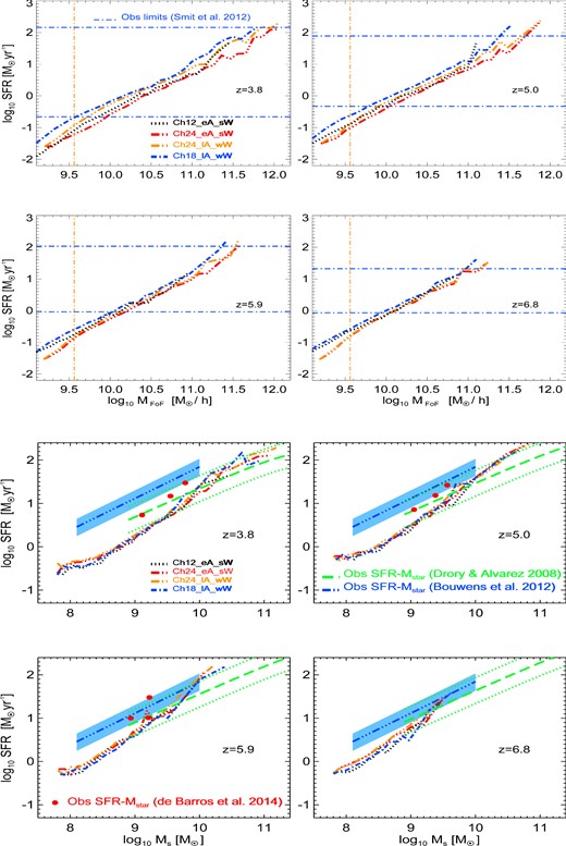
Box size and resolution tests at redshift z ∼ 4–7. Top foue panels: SFR–MFoF relation. Bottom four panels: SFR–M⋆ relation. In all the panels, we compare (a) the Chabrier IMF, Early AGN, Strong winds configuration for two different box sizes: L = 24 Mpc h−1 (Ch24_eA_sW – red triple dot–dashed line) and L = 12 Mpc h−1 (Ch12_eA_sW - black dotted line) and (b) the Chabrier IMF, Late AGN, Weak Winds configuration for L = 24 Mpc h−1 (Ch24_lA_wW – orange triple dot–dashed line) and L = 18 Mpc h−1 (Ch18_lA_wW – blue dot–dashed line). In the top four panels, the blue dot–dashed horizontal lines represent the observational limits in the range of SFR of Smit et al. (2012) and the orange dot–dashed vertical line is our mass confidence limit (see Section 3.1). In the bottom 4 panels, we overplot the observed galaxy SFR(M⋆) relations from Drory & Alvarez (2008, observed frame I-band selected sample – green dashed + dotted lines), Bouwens et al. (2012, droup-outs selection – blue triple dot–dashed lines + light blue shaded regions) and de Barros et al. (2014, droup-outs selection – nebular emission – red filled circles).
In the bottom four panels of Fig. 12, we test the SFR–M⋆ relation using the same simulations. In this case, there is a very good agreement between the different runs at all redshifts considered. For comparison, we overplotted the observations of Drory & Alvarez (2008, observed frame I-band selected sample – green dashed + dotted lines), Bouwens et al. (2012, droup-outs selection – blue triple dot–dashed lines + light blue shaded regions) and de Barros et al. (2014, droup-outs selection – nebular emission – red filled circles).
In Fig. 13, we plot the GSMFs for the four runs used before and we compare with the observational results of Marchesini et al. (2009, green filled circles with error bars), González et al. (2011, blue filled squares with error bars) and Santini et al. (2012, magenta dashed line). The effect of poorer statistics at high stellar masses for the Ch12_eA_sW run is clearly visible. However, in each panel our simulations show a good convergence down to the observational point of González et al. (2011) at log (M⋆/M⊙) = 8.25. Below this limit, incompleteness effects, due to the SFR/mass cut we adopted in our simulations, start to be important (the same feature is visible for the runs plotted in Figs 9, 10 and 11).
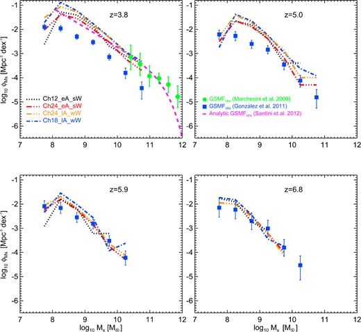
Box size and resolution tests: galaxy stellar mass functions at redshift z ∼ 4–7. We compare the same simulations of Fig. 12 (line-styles of different simulations are also the same). Overplotted are the observational results of Marchesini et al. (2009, green filled circles with error bars), González et al. (2011, blue filled squares with error bars) and Santini et al. (2012, magenta dashed line).
To summarize, the SFR–M⋆ relation converges at 4 ≤ z ≤ 7, while the SFR–MFoF relation shows a slightly worse convergence at z = 5.0. Finally, at all redshifts considered the GSMF converges down to log (M⋆/M⊙) = 8.25.
