


Abstract
We present a new N-body simulation from the Marenostrum Institut de Ciències de l'Espai (MICE) collaboration, the MICE Grand Challenge (MICE-GC), containing about 70 billion dark matter particles in a (3 Gpc h−1)3 comoving volume. Given its large volume and fine spatial resolution, spanning over five orders of magnitude in dynamic range, it allows an accurate modelling of the growth of structure in the universe from the linear through the highly non-linear regime of gravitational clustering. We validate the dark matter simulation outputs using 3D and 2D clustering statistics, and discuss mass-resolution effects in the non-linear regime by comparing to previous simulations and the latest numerical fits. We show that the MICE-GC run allows for a measurement of the BAO feature with per cent level accuracy and compare it to state-of-the-art theoretical models. We also use sub-arcmin resolution pixelized 2D maps of the dark matter counts in the lightcone to make tomographic analyses in real and redshift space. Our analysis shows the simulation reproduces the Kaiser effect on large scales, whereas we find a significant suppression of power on non-linear scales relative to the real space clustering. We complete our validation by presenting an analysis of the three-point correlation function in this and previous MICE simulations, finding further evidence for mass-resolution effects. This is the first of a series of three papers in which we present the MICE-GC simulation, along with a wide and deep mock galaxy catalogue built from it. This mock is made publicly available through a dedicated web portal, http://cosmohub.pic.es.
1 INTRODUCTION
These are exciting times for cosmology. The new generation of astronomical surveys will deliver a detailed picture of the universe, providing a better understanding of the galaxy formation process and determining whether General Relativity correctly describes the observables that characterize the expansion rate of the universe and the growth of large-scale structures. In particular, one of the main science goals of upcoming galaxy surveys is to pin down the properties of the dark energy that drives the observed accelerated expansion of the universe.
In order to answer these key questions, we need to interpret astronomical data sets with high precision. Given the difficulty of the problem, N-body simulations have become a fundamental ingredient to develop mock cosmological observations, by providing a laboratory for the growth of structure under the only effect of gravity. However, the ever increasing volume and complexity of observational data sets demand a matching effort to develop larger and higher accuracy cosmological simulations.
In this paper, we present a new N-body simulation developed by the Marenostrum Institut de Ciències de l'Espai (MICE) collaboration at the Marenostrum supercomputer, the MICE Grand Challenge run (MICE-GC), that includes about 70 billion dark matter particles, in a box of about 3 h−1 Gpc aside. This simulation samples from the largest (linear) scales accessible to the observable universe, where clustering statistics are Gaussian, down to the highly non-linear regime of structure formation where gravity drives dark matter and galaxy clustering away from Gaussianity. We build halo and galaxy catalogues in order to help the design and exploitation of new wide-area cosmological surveys. We present several applications of this large cosmological simulation for 2D and 3D clustering statistics of dark matter in comoving outputs and in the lightcone.
One of the main focus of this paper is to investigate the impact of mass-resolution effects in the modelling of dark matter and galaxy clustering observables by comparing the MICE-GC, and previous MICE runs, to analytic fits available based on high-resolution N-body simulations. For this purpose, we have thoroughly analysed the simulation outputs using basic 3D and 2D clustering statistics in comoving outputs and in the lightcone. We show that our results are consistent with previous work in linear and weakly non-linear scales, and show how the new simulation better samples power on small-scales, described by the highly non-linear regime of gravitational clustering.
This paper is the first of a series of three introducing the MICE-GC end-to-end simulation, its validation and several applications. Paper I (i.e. this paper) presents the MICE-GC N-body lightcone simulation and its validation using dark matter clustering statistics. The halo and mock galaxy catalogue, along with their validation and applications to abundance and clustering statistics are presented in Crocce et al. (2013, hereafter Paper II). The all-sky lensing maps and the inclusion of lensing properties to the mock galaxies are discussed in Fosalba et al. (2013, hereafter Paper III).
Accompanying this series of papers, we make a first public data release of the MICE-GC lightcone galaxy mock (MICECAT v1.0) through a dedicated web portal for simulations: http://cosmohub.pic.es, where detailed information on the data provided can be found. We plan to release improved versions of the MICE galaxy mocks through this web portal in due time.
This paper is organized as follows: Section 2 presents the MICE-GC simulation and how it compares to state-of-the-art in the field of numerical simulations in cosmology. In Section 3, we validate the dark matter outputs of the simulation using the 3D matter power spectrum, and its Fourier transform, the two-point correlation function (i.e. 2PCF). In Section 4, we investigate the distribution of dark matter in the all-sky lightcone by means of 2D pixelized maps. We focus in the clustering of projected dark matter counts in redshift bins in real and redshift space using the angular power spectrum and its Legendre transform, the angular two-point correlation function (A2PCF). We compare these results to previous simulations and available numerical fits. Section 5 presents an analysis of the three-point correlation function of the dark matter comoving outputs in the MICE-GC, and compares it to previous MICE runs and theory predictions. Finally, in Section 6 we summarize our main results and conclusions.
2 THE MICE GRAND CHALLENGE SIMULATION
We have developed a set of large N-body simulations with gadget-2 (Springel 2005) on the Marenostrum supercomputer at BSC.1 We shall name them MICE simulations hereafter. Further details about the MICE simulations can be found in the project website, www.ice.cat/mice.
In this paper, we shall focus on the MICE Grand Challenge simulation (MICE-GC hereafter). This simulation contains 40963 dark matter particles in a box-size of Lbox = 3072 h−1 Mpc, and assumes a flat concordance LCDM model with Ωm = 0.25, |$\Omega _\Lambda =0.75$|, Ωb = 0.044, ns = 0.95, σ8 = 0.8 and h = 0.7, consistent with the best-fitting cosmology to WMAP five-year data (Dunkley et al. 2009). The resulting particle mass is mp = 2.93 × 10¹⁰ h−1 M⊙ and the softening length used is, lsoft = 50kpc h− 1. We start our run at zi = 100 displacing particles using the Zeldovich dynamics. The initial particle load uses a cubic mesh with 40963 nodes. The entry Max. Time-step in Table 1 is the initial global time-stepping used, which is of the order of 1 per cent of the Hubble time (i.e, d log a = 0.01, being a the scale factor). The number of global time-steps to complete the run was Nsteps ≳ 3000, and we write the lightcone on-the-fly in 265 steps from z = 1.4 to 0.
Description of the MICE N-body simulations. Npart denotes number of particles, Lbox is the box-size, PMGrid gives the size of the Particle-Mesh grid used for the large-scale forces computed with FFTs, mp gives the particle mass, lsoft is the softening length, and zin is the initial redshift of the simulation. All simulations had initial conditions generated using the Zeldovich Approximation. Max. Time-step is the initial global time-stepping used, which is of the order of 1 per cent of the Hubble time (i.e, d log a = 0.01, being a the scale factor). The number of global time-steps to complete the runs were Nsteps ≳ 2000 in all cases, except for the MICE-GC which took ≳ 3000 time-steps. Their cosmological parameters were kept constant throughout the runs (see text for details).
| Run | Npart | Lbox/ h−1 Mpc | PMGrid | mp/(1010 h−1 M⊙) | lsoft/ h−1 Kpc | zi | |${\rm Max. Time{\rm -}step}$| |
|---|---|---|---|---|---|---|---|
| MICE-GC | 40963 | 3072 | 4096 | 2.93 | 50 | 100 | 0.02 |
| MICE-IR | 20483 | 3072 | 2048 | 23.42 | 50 | 50 | 0.01 |
| MICE-SHV | 20483 | 7680 | 2048 | 366 | 50 | 150 | 0.03 |
In Table 1, we describe the gadget-2 code parameters used in the MICE simulations discussed in this paper: the MICE-GC, the Intermediate Resolution (MICE-IR; Fosalba et al. 2008) and the Super-Hubble Volume (MICE-SHV; Crocce et al. 2010).
We construct a lightcone simulation by replicating the simulation box (and translating it) around the observer, thus allowing us to build all-sky lensing outputs with negligible repetition up to zmax = 1.4. The methodology used to develop all-sky (spherical) lightcone outputs is described in (Fosalba et al. 2008), where further details are given on how the all-sky lensing maps in the Born approximation are constructed using pixelized 2D projected dark matter density maps. Fig. 1 shows an image of the all-sky lightcone at z = 0.6. The nested zooms illustrate the wide dynamic range sampled by the simulation. In particular, thanks to its combination of large volume and good mass resolution, the MICE-GC simulation is able to sample from the largest (linear) scales encompassing nearly all the observable universe down to fairly small (non-linear) scales with few per cent accuracy, as we shall show in this work.
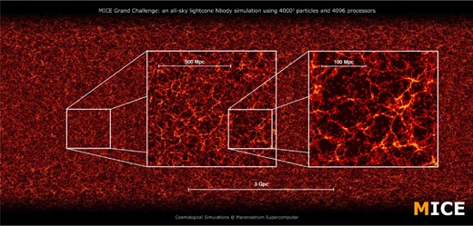
MICE-GC dark matter lightcone simulation at z = 0.6. The image shows the wide dynamic range, about five decades in scale, sampled by this N-body simulation.
A particularly challenging aspect of any large-volume cosmological simulation is the ability to accurately sample small-scale (non-linear) power while still sampling a large volume. This ability is determined by the particle mass (or density of particles) in the simulated volume. In what follows, we shall refer to the impact of the particle mass on clustering observables as mass-resolution effects.
In this paper, we introduce this new very large cosmological simulation as a powerful tool to model accurately current and upcoming deep wide-area astronomical surveys such as DES,2 HSC,3Euclid,4 DESI,5 HETDEX,6 LSST,7 WFIRST,8 among others.
We test the ability of MICE-GC to model these large surveys on the smaller scales and to what extent it resolves the small-mass haloes inhabited by the faintest galaxies these surveys will observe. Fig. 2 shows how MICE-GC compares to the largest simulations currently available in performance to sample large cosmological volumes and capture, at the same time, low enough luminosity galaxies Lmin, or equivalently, large enough r-band absolute magnitude Mr. The relation between minimum halo mass and minimum galaxy luminosities modelled, as shown in the figure, assumes a sub-halo abundance matching galaxy assignment scheme on well-resolved dark matter haloes containing at least 100 particles. We show the following simulations: Millennium XXL (MXXL; Angulo et al. 2012), Horizon Runs (HR; Kim et al. 2009, 2011), Horizon Simulation (HS; Teyssier et al. 2009), DEUSS (Alimi et al. 2012), Jubilee (Watson et al. 2014), BigMultiDark(Klypin et al. 2013), MICE Intermediate Resolution (MICE-IR; Fosalba et al. 2008), MICE Super-Hubble-Volume (MICE-SHV; Crocce et al. 2010) and the MICE-GC simulation.
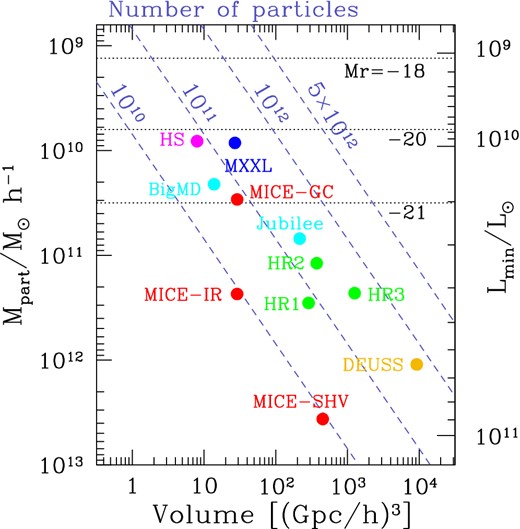
State-of-the art in cosmological simulations: performance in terms of survey volume and particle mass, or equivalently, faintest Lmin galaxy luminosity (or absolute magnitude in r band) reached according to an HOD galaxy assignment scheme to populate haloes with 100 or more dark matter particles.
This suite of simulations includes numbers of particles that span from about 10 billion up to 1 trillion particles, already accessible in the largest supercomputers around the world. This figure shows the trade-off between high mass resolution and large volume sampling what tends to distribute the most competitive simulations to date along the dashed lines shown, depending on the number of particles used. As shown in Fig. 2, the MXXL is the state-of-the art cosmological simulation in terms of sampling as large a volume as possible with a high mass resolution. Our simulation compares well to it, as it has a comparable volume (3.072 Gpc h−1) and only four times lower mass resolution (2.93 × 10¹⁰ h−1 M⊙).
As an example, in order to resolve Mr = −18 galaxies one would need to develop a simulation with a (4 Gpc h−1)3 box-size that includes about five trillion particles (i.e. 163843). This is one order of magnitude larger than the MXXL and almost two orders of magnitude bigger than e.g. the MICE-GC, which are among the largest simulations completed to date.
3 3D CLUSTERING
3.1 Power spectrum
One of our main goals is to study the large-scale clustering with high precision, in particular the baryon acoustic oscillations (BAO). Hence Fig. 3 shows the matter 3D power spectrum measured in MICE-GC at large (BAO) scales for three comoving outputs, z = 0, 0.5 and 1 (divided by a smooth broad-band power). For comparison we included linear theory, the renormalized perturbation theory (RPT) prediction as presented in Crocce & Scoccimarro (2008), and the numerical fits from (Heitmann et al. 2014, i.e. the Coyote Emulator) and Takahashi et al. (2012), which we shall name the revised halofit. The prediction from RPT at two-loops reproduces very well the region of BAO, thus cross-validating the modelling and the N-body precision in describing this feature. We find the Coyote Emulator to give a good description of the overall BAO features in our run, but with a systematic 2 per cent excess (broad-band) amplitude at z = 0.5, 1. The revised Halofit yields a similar level of agreement but in that case the amplitude of the oscillatory features appear too large.
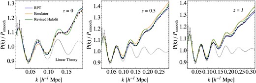
BAO measured in MICE-GC (black symbols with error bars) power spectrum compared to the theory prediction from RPT (blue line; see Crocce & Scoccimarro 2008) and the latest numerical fit from the Coyote Emulator (orange line; Heitmann et al. 2014) and the revised Halofit (green line; Takahashi et al. 2012). The RPT model at two loops reproduces very well the BAO in the simulation across redshifts (each panel is shown up to the maximum k where RPT is valid). In turn at z = 0 the Emulator yields a very good match with MICE-GC (except for the amplitude of the first peak with a difference ≲ 2 per cent). At z = 0.5, 1 the broad-band power has the correct shape but is 2 per cent (systematically) above the N-body. The revised halofit also agrees with MICE-GC at the 2 per cent level at these redshifts but the amplitude of the oscillations are somewhat too large. Displayed error bars assume Gaussian fluctuations, |$\sigma _P = \sqrt{2/n_{\rm modes}} P_k$|, but we take Pk to be the non-linear spectrum (see text).
In turn, Fig. 4 shows the MICE-GC two-point clustering measurements in the transition to the highly non-linear regime and how they compare to the revised Halofit and the Coyote Emulator on those scales.9 Different panels correspond to different comoving outputs, namely z = 0, 0.5, 1 and 1.5 (top to bottom). As discussed above the Emulator is systematically above our measurement on scales k ≲ 0.3 h Mpc−1 by about 2 per cent (for z > 0). Towards smaller scales we find a pronounced jump in the prediction at intermediate redshifts and k ∼ 0.3–0.4 h Mpc−1 of ∼3 per cent. The overall matching with MICE-GC measurements stays at the level of ±2 per cent up to k ∼ 1 h Mpc−1. The revised Halofit is slightly above our measurements across scales, but particularly at the ‘one-halo’ regime beyond k ∼ 0.3 h Mpc−1, where differences rise to about 5–8 per cent depending on redshift. In Fig. 4, and following the discussion after equation (1), we display 1 and 3 σ error bars with shaded regions using equation (1) for k ≤ 0.4 h Mpc−1 and its value (σP/P)|k = 0.4 for k ≥ 0.4 h Mpc−1.

Matter power spectrum in MICE-GC at several comoving outputs compared to the latest available numerical fits, the revised Halofit (Takahashi et al. 2012) and the Coyote Emulator (Heitmann et al. 2014). The shaded regions show the 1σ and 3σ error bars given the box-size and the binning (see text for details). The overall matching with the emulator is at the level of 2 per cent (but systematically below), with a jump of ≲ 3 per cent at k ∼ 0.3–0.4 h−1 Mpc. In turn, the revised Halofit overpredicts the power on small scales by 5 to 8 per cent (see text for a more detailed discussion). Vertical arrows show BAO peaks for reference.
We should note that on small scales (k ∼ 1 h Mpc−1) our run might suffer from per cent level systematics effects that could impact the discussion above. For example setting the size of the Particle-Mesh grid (the PMGrid parameter) equal to the number of particles (as done in MICE-GC, see Table 1), instead of larger, can yield excess power on quasi-linear scales of ≲ 1 per cent (Smith et al. 2014). In turn, transients from initial conditions suppress power on these scales. For MICE-GC, with zi = 100, we expect this to be a small effect none the less. For an order of magnitude, we have estimated the relative transient effect (i.e. P(k, zi = 100)/P(k, zi = ∞)) using perturbation theory (PT, see fig. 6 in Crocce, Pueblas & Scoccimarro 2006) and found an ∼(1–1.5) per cent effect at scales k ∼ 0.5–1 h Mpc−1.
We next turn to discuss the impact of particle mass resolution in the generation of non-linear structure by comparing the clustering in MICE-GC to that in MICE-IR, a factor of 8 worse resolution run. This lower resolution simulation was already presented and extensively validated in Fosalba et al. (2008), and Crocce et al. (2010).10 We note that both simulations were done with almost the same run parameters (see Table 1) with the main difference being the initial transfer function. MICE-IR used the Eisenstein & Hu (EH from now on) approximation (Eisenstein & Hu 1998) while MICE-GC used an (exact) camb output.11 The differences between these two initial spectra, shown in the top panel of Fig. 5, are however very small: ≲ 4 per cent at BAO positions and within 2 per cent up to k ∼ 50 h Mpc−1 (although only k < 1 h Mpc−1 is plotted).
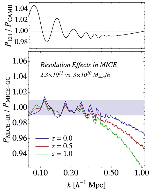
Top panel: ratio of the initial EH linear power spectrum used in MICE-IR to the one used in MICE-GC from camb, both for the same (MICE) cosmology. Bottom panel: suppression of non-linear structure formation due to particle mass resolution seen through the ratio of the power spectrum measured in MICE-IR (mp ∼ 2.3 × 10¹¹ h−1 M⊙) to the one in MICE-GC (mp ∼ 3 × 10¹⁰ h−1 M⊙) at z = 0, 0.5 and 1. MICE-IR measurements were corrected assuming a Poisson shot-noise and the slight difference in initial spectra was divided out. If we do not correct for shot-noise, we find these ratios to be almost independent of redshift and to resemble the z = 0 case shown by the blue line.
The resolution study is given in the bottom panel of Fig. 5. It shows that the non-linear power spectrum measured in MICE-IR is suppressed compared to that in MICE-GC, by 3, 5 and ∼8 per cent at k = 1 h Mpc−1 and z = 0, 0.5 and 1, respectively. These differences are somewhat expected because particle mass resolution impacts how well small-scale power is sampled from the simulated dark matter distribution. The lower the particle mass, the better small scales are sampled. In the language of the halo model, a smaller particle mass is able to resolve smaller mass haloes that contribute to the power spectrum on correspondingly smaller scales. Notice that the effect can be significant even on rather large scales (1–2 per cent at k ∼ 0.4 h Mpc−1). In Fig. 5, the MICE-IR power spectra have been corrected for finite particle number assuming a Poisson shot-noise (while MICE-GC has negligible noise on these scales). If we have not done so the P(k) ratio at different redshifts would have resembled the z = 0 case in Fig. 5, i.e. a resolution effect being ∼2–3 per cent at k = 1 h Mpc−1. One difference between the simulation runs that can impact part of the effect shown in Fig. 5 is the starting redshift. Because MICE-IR started at a lower redshift than MICE-GC (zi = 50 versus zi = 100, respectively), its clustering is expected to be suppressed at non-linear scales. However, we have estimated this to be a 1 per cent effect in the k range 0.5–1 h Mpc−1 for the redshifts shown (using PT; see Crocce et al. 2006).
3.2 Two-point correlation function
To complement the previous sections, we show in left-hand panel of Fig. 6 the spatial correlation function of dark matter particles in the z = 0 comoving output of MICE-GC. This is basically the Fourier counterpart of Fig. 3 but it is still interesting to see how any mismatch between the measurements and the theory in that figure translate to configuration space. The BAO wiggles from the revised Halofit (Takahashi et al. 2012) which are too pronounced in Fourier space also yield the wrong amplitude for the correlation turnover at ∼90 h−1 Mpc and the BAO peak at 110 h−1 Mpc. Both RPT (Crocce & Scoccimarro 2008) and Coyote (Heitmann et al. 2014) seem to agree better with MICE-GC. All models agree very well with themselves and the measurements on smaller scales, 20 h−1 Mpc ≤ r ≤ 70 h−1 Mpc. For concreteness, we focused on z = 0.5 but similar conclusions are reached for z = 0 and 1.
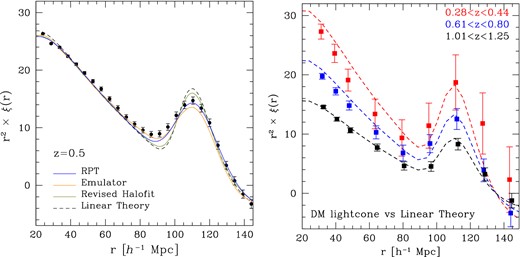
Left-hand panel: dark matter correlation function in MICE-GC at z = 0.5 at large scales (the Fourier counterpart to the middle panel of Fig. 3). We include the Fourier transform of the models shown in Fig 3: RPT (blue; Crocce & Scoccimarro 2008), Emulator (orange; Heitmann et al. 2014), the revised Halofit (green; Takahashi et al. 2012) and linear theory (dashed black). The latter is the one that shows the worse agreement with our N-body at BAO scales (in the amplitude of the feature), while RPT and Emulator are in better agreement. Similar conclusions are reached at z = 0 and 1. Right-hand panel: corresponding results for difference redshift slices over one octant of the MICE-GC lightcone output (also in real space) smoothed over 8 h−1 Mpc pixels and 16 h−1 Mpc bins in pair separation r. Dashed lines are the smoothed linear theory predictions (which resemble non-linear predictions). Note how the errors are larger (and more realistic) because of the smaller volume available in the lightcone.
Right-hand panel of Fig. 6, shows the correlation function measurements for different redshifts in the lightcone. The top-hat filter is a cubical cell of side 8 Mpc h−1. We split the correlation in bins of 16 Mpc h−1 to reduce the error bars. So the smoothing is not necessary, but it speeds up the codes, which are the same as we use for the three-point correlation, for which the execution time reduction is critical. The redshift bin is given in complete cell sizes which also reduces the impact of the boundaries. The redshifts depth could add some effects due to selection in redshift space, but we have checked that mean results do not change much (within errors) for other bin widths. This smoothing makes the linear and non-linear results look quite closer on BAO scales. On the largest scales there is good agreement, within the errors, with the linear theory predictions (dashed lines), especially at the larger redshifts. At the lower redshifts, non-linear effects are more important (distorting the shape of the BAO peak and the amplitude around r ≃ 40–80 h−1 Mpc) and errors are larger because of the smaller volume in the lightcone. Given these errors and the smoothing, it is hard to evaluate if there are additional lightcone distortions in addition to the non-linear effects that we find in the comoving outputs.
4 ANGULAR CLUSTERING IN THE LIGHTCONE
Following the approach presented in Fosalba et al. (2008), we construct a lightcone simulation by replicating the simulation box (and translating it) around the observer. Given the large box-size used for the MICE-GC simulation, Lbox = 3072 h−1 Mpc, this approach allows us to build all-sky lightcone outputs without significant repetition up to zmax = 1.4. Then we decompose the lightcone volume, in the range 0 < z < 1.4, into a set of 265 all-sky concentric spherical (or radial) shells around the observer, with a constant width of ∼70 Mega-years in lookback time. This width corresponds to about 8 Mpc h−1 at z ≃ 0 and 15 Mpc h−1 at z ≃ 1.4. Lightcone outputs are written on the fly for each of these spherical shells. We linearly interpolate particle positions using their velocities at the lightcone time-step or radial shell.
4.1 Angular clustering in real space
Fig. 7 shows the angular power spectrum for all-sky projected dark matter overdensity in narrow redshift slices, for the MICE-GC, compared to a previous lower mass resolution run, the MICE-IR. Particle shot-noise, shown as solid lines at the right of the upper panels, has been subtracted from the measured power spectra and displayed theoretical error bars correspond to an (ideal) all-sky survey. Throughout this paper, we shall use Gaussian theoretical error bars for the different observables of 2D clustering, unless otherwise stated, following Cabre et al. (2007), Crocce, Cabré & Gaztañaga (2011a). We shall stress that this is an optimistic error estimate on small scales, since a significant deviation from the Gaussian approximation is expected to arise as a result of non-linear gravitational growth (Scoccimarro, Zaldarriaga & Hui 1999).
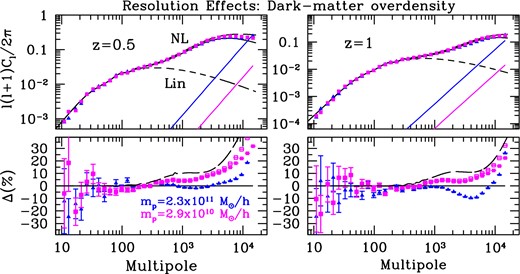
Angular power spectrum of the projected dark matter overdensity field in redshift (all-sky lightcone) slices. Left-hand panels show power spectra for a broad z-bin slice at z = 0.5 and Δz = 0.1, whereas the right-hand panels show the case for z = 1 with the same bin width. Dashed and solid lines show linear theory and non-linear fit (Halofit) predictions, respectively. Long dashed lines shows the revised Halofit (Takahashi et al. 2012) which shows a clear excess of power with respect to the old Halofit (Smith et al. 2003). Symbols show measurements from simulations and the solid lines at the bottom right display the estimated shot-noise levels. Lower panels show relative deviations with respect to the old Halofit prediction. For clarity, in these lower panels, we only show power spectra both with (open symbols) and without (filled symbols) shot-noise for the MICE-GC simulation, where shot-noise does not affect small-scale power significantly. Mass-resolution effects at the 20–30 per cent level are observed for multipoles ℓ > 103.
As shown in the lower panels of Fig. 7, using a particle mass eight times lower, produces a drop in the measured power at the 5 per cent level for multipoles ℓ ∼ 103, which corresponds to wavenumbers k ∼ 0.75 at z = 0.5 and k ∼ 0.5 for z = 1 in the flat-sky (or Limber) limit. The impact of such mass-resolution effect is even larger for higher redshift. This is consistent with the effect seen in the 3D power spectrum (see Fig. 5). The fact that the magnitude of mass-resoution effects (and its dependence with redshift) at these quasi-linear scales are consistent in 3D comoving versus 2D lightcone outputs implies that possible lightcone artefacts (e.g, interpolation issues between lightcone time-steps) do not affect our results. For even smaller scales (103 < ℓ < 104) the difference rises up to 10–20 per cent, although here the amplitude of the effect and its scale-dependence start to be sensitive to the details of the shot-noise correction. Besides, at these highly non-linear scales, we cannot exclude possible lightcone interpolation artefacts, but again these would be difficult to separate from other sources of error such as inaccurate shot-noise correction. Comparing to state-of-the-art numerical fits, the MICE-GC measurements in the range 103 < ℓ < 104 show an 5–10 per cent excess relative to Halofit (Smith et al. 2003), and a 5–10 per cent deficit with respect to the revised Halofit by Takahashi et al. (2012), based on small-box high-resolution N-body simulations. This trend of increasing power excess as one uses higher resolution simulations indicates that what we observe on these scales is also consistent with the impact of mass resolution on the clustering.
Any inconsistency in the parameters used for the simulations compared above could question the robustness of our conclusions. In particular, MICE-GC which uses the exact transfer function (computed with camb) to generate the initial conditions, whereas MICE-IR employs the EH approximation to the exact transfer function. However, differences between the exact and EH power spectrum are typically within 2 per cent for k ≲ 10, which corresponds to multipoles ℓ ≲ 104 for z > 0.5. Therefore, the observed discrepancy in the angular power spectra cannot be attributed to this slight inconsistency in the initial conditions. Other effects on this ℓ range, such as transients from initial conditions (see Crocce et al. 2006), are expected to have a negligible impact for the MICE-GC outputs on these scales, but a detailed discussion will be presented elsewhere.
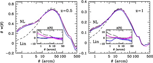
Same as Fig. 7 but for the A2PCF. In order to better compare to theory predictions, we use lines (instead of symbols) to display MICE-GC measurements. The inset panels display the ratio of measurements (and revised halofit) to the Smith et al. (2003) halofit prediction. We zoom into smaller angular scales to highlight mass-resolution effects.
In a similar manner mass-resolution effects are found to be smaller by roughly a factor of 2 in the A2PCF with respect to the angular power spectra for the same redshift bins and corresponding angular scales if the 1-to-1 relation would hold (see Figs 7 and 8). We find a 5–10 per cent and 10–20 per cent effect for w(θ) and the Cℓ's, respectively, for broad redshifts bins in the range z = 0.5–1. On the other hand on linear scales, θ ≳ 30–60 arcmin depending on redshift, MICE-IR results clearly deviate from those of MICE-GC (and theory predictions). This can be due to a good extent to the different transfer function used to set up the initial conditions in both simulations. As shown in Fig. 5, there are ≳ 4 per cent differences between the initial power spectra of these two MICE simulations at k ≲ 0.1 h Mpc−1, what corresponds to angular scales of θ = 180°/(kr(z)) ≃ 80 and 45 arcmin, in the Limber or small-angle limit, for z = 0.5 and 1, respectively.
4.2 Angular clustering in redshift space
In this section, we discuss the impact of peculiar velocities (or redshift space distortions) in the angular power spectra and correlation function of dark matter overdensities. Redshift space distortions (RSD) do not change the angular position of a single galaxy, nor they change significantly its measured redshift in photometric surveys. However, the coherent large-scale motions present in RSD can have a large impact on the net angular correlation in a sample of galaxies. In particular, when the boundaries of the galaxy sample are defined in redshift space (as it happens in a real survey) then large-scale motions move structures across the boundaries in a spatially coherent way. In particular, the so-called Kaiser effect (Kaiser 1987) produces a large enhancement of the resulting angular correlations (see e.g. Crocce et al. 2010; Nock, Percival & Ross 2010). Although the use of photometric redshifts tends to counteract the correlations enhancement due to RSD by smoothing the 2PCF, the impact of RSD is still measurable in photometric surveys. This impact is seen as a net enhancement of the correlations measured in photometric surveys with respect to that expected in real space, and depends on the particular choice of redshift bin width, being larger for narrower bins (as shown in our Figs 9 and 10 below, or fig. 5 in Crocce et al. 2011).
Below we shall model RSD for both broad and narrow redshift bin widths. The former is important for research that aims at measuring the growth of structure through RSD in photometric surveys (Padmanabhan et al. 2007; Crocce et al. 2011b; Ross et al. 2011; Asorey, Crocce & Gaztanaga 2014). The latter scenario is very relevant for recent studies that combine RSD in spectroscopic surveys with weak gravitational lensing, to break degeneracies between bias and dark energy parameters (Gaztañaga et al. 2012; de Putter, Doré & Takada 2013; Font-Ribera et al. 2014; Kirk et al. 2013).
Let us start by comparing the angular power spectrum in lightcone dark matter outputs in real and redshift space from large linear scales (i.e low multipoles) to small and non-linear scales (high multipoles). In Fig. 9, we show results for dark matter sources in the lightcone at mean redshifts, z = 0.5 and 1. In order to see the impact of projection effects, we display results for two cases, broad Δz = 0.1 (left-hand panels) and narrow Δz = 0.01 (right-hand panels) redshift bins. Theory predictions, computed with camb sources, are given in the linear and non-linear regime for the growth of structure (Halofit, solid lines). However, theory RSD effects are only computed in the linear regime, the so-called Kaiser effect.
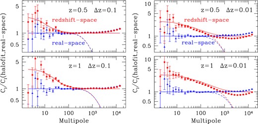
Comparison between angular clustering in real and redshift space. Left-hand panels show results for z = 0.5, 1 for two broad redshift bins, Δz = 0.1. Theory predictions are given in the linear (dashed) and non-linear regime of gravitational clustering (Halofit, solid lines). Theory RSD effects are only modelled in the linear regime (i.e. Kaiser effect), following the camb implementation. Symbols display measurements in the MICE-GC simulation. Both theory and simulation results are normalized to non-linear theory predictions in real space (labelled ‘halofit, real-space’ in the figures). Simulations show that RSD effects enhance the large-scale (low-ℓ) clustering relative to real space, by a factor of ≃ 3, in agreement with linear predictions (red lines). Non-linear RSD tend to suppress power on small scales. This is only significant in 2D clustering for sufficiently narrow redshift bins, e.g, Δz = 0.01 (see right-hand panels).
In Fig. 9, both theory and simulation results are normalized to the non-linear Halofit (Smith et al. 2003) predictions in real space (labelled ‘halofit, real-space’ in plots). Simulations show that RSD effects enhance the large-scale (low-ℓ) clustering relative to real space, by a factor of ≃ 3 (although it depends slightly on redshift), in agreement with the Kaiser effect (e.g. Padmanabhan et al. 2007). This is also clearly seen in configuration space, see Fig. 10, where simulations accurately recover the Kaiser ‘boost’ for angular scales θ ≳ 50–100 arcmin. In particular, the Kaiser boost also enhances the BAO feature on few degree angular scales, an effect that has been studied in depth in the context of upcoming photometric surveys (Crocce et al. 2010; Nock et al. 2010).
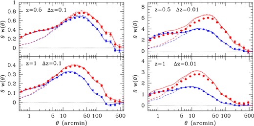
Same as Fig. 9 but for the angular 2PCF. The theory predicted Kaiser effect is recovered in the simulation for θ ≳ 50–100 arcmin, where coherent motions of dark matter particles tend to enhance clustering by a factor, ≃ 3. For narrow z-bins (right-hand panels) non-linear RSD appear at θ ≲ 100 arcmin, where the simulation (red symbols) deviates from linear RSD theory (red solid lines).
Alternatively, non-linear RSD effects in the 2PCF w(θ) are significant on scales θNL-RSD ≲ 100 arcmin. In analogy to what we found in harmonic space, this angular scale is roughly an order of magnitude larger than the transition scale to non-linear gravitational growth, θNL-growth ≃ θNL-RSD/10 ≃ 10 arcmin, as shown in Fig. 10. The amplitude of non-linear RSD effects, estimated as the difference between the linear RSD theory prediction (red solid line) and the simulation measurement (red symbols) on θ < θNL-RSD, is ≃ 2 per cent on non-linear scales for the broad z-bin, Δz = 0.1, and up to ≃ 5–15 per cent for scales θ = 60 − 1 arcmin, respectively, for the narrow z-bin. These amplitudes are in agreement with the results found for the angular power spectra at the highest multipoles (i.e. non-linear scales), Fig. 9.
5 HIGHER ORDER CLUSTERING: three-POINT CORRELATION FUNCTION
5.1 Mass-resolution effects
To illustrate the dependence of Q3 on the triangle shape we will fix two of the triangle sides (r12, r13) and display results as function of the third side r23. Fig. 11 shows a comparison of Q3 as measured from the MICE simulations of different particle resolutions. We also show the predictions from tree-level PT (from Barriga & Gaztañaga 2002) using different transfer functions in the initial conditions (i.e. camb and EH) and the no-wiggle model of EH, i.e. without the BAO peak. We have found very little change of Q3 with redshift within the errors, so these results are very similar for 0 < z < 1 (see also Fig. 14 below).
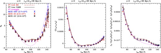
Reduced three-point Q3(r12, r13, r23) (left-hand panel), which is the ratio, see equation (7), of the three-point ζ(r12, r13, r23) (middle panel) to the hierarchical two-point product ζH ≡ ξ(r12)ξ(r23) + ξ(r12)ξ(r13) + ξ(r23)ξ(r13) (right). This is for z = 0 and r13 = 2r12 = 96 Mpc h−1, as a function of r23. MICE simulations of different resolutions (as labelled in the top panel) are compared to PT results with different IC (transfer functions), including the case without BAO (no-wiggles). The BAO peak can be clearly seen as a bump around 110 h−1 Mpc in all panels. A lack of resolution reduces the power in the two-point ζH, but increases slightly the anisotropy in the three-point ζ. Both effects makes Q3 significantly more anisotropic as we reduce the mass resolution in the MICE simulations.
We can see a small, but systematic and significant, dependence on the simulation mass particle resolution that are comparable in order of magnitude to the deviations between simulations and PT and also the differences between different transfer functions. The biggest discrepancy is with the model without a BAO, indicating that the BAO can be clearly detected in Q3 in our simulations (see Gaztañaga et al. 2009 and references therein for measurements of this effect). These results can only be achieved with the largest volumes (and therefore at higher redshifts in the lightcone).
The discrepancies at the two-point function level, i.e. in ζH, are comparable to what we show in previous sections and can be understood using the halo model. The higher the resolution the lower the mass haloes that we can resolve. This results in higher power on the smallest scales, corresponding to the smallest mass haloes that are resolved. For the three-point function, the effect comes from the mode coupling which makes the clustering anisotropic. This results in a characteristic anisotropic shape of Q3 or ζ as a function of the triangle shape (which is given by a U-Shape as a function of r23 in Fig. 11). Non-linear dynamics tend to reduce this shape dependence and makes clustering more isotropic, especially on the smaller scales (e.g. see Bernardeau et al. 2002). This could explain why a better resolution of non-linear effects (which comes with higher particle resolution) results in slightly more isotropic clustering, which in our case means slightly lower amplitudes of Q3 and ζ for elongated triangles, as shown in Fig. 11.
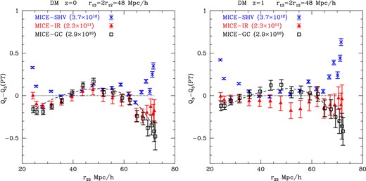
The difference between leading order PT results and measurements in simulations with different resolutions. In each case, we use the corresponding transfer function to estimate the PT results. This is for triangles with r13 = 2r12 = 48 Mpc h−1 and shown as a function of the remaining leg r23. As the simulation evolves the different resolution converge to each other (left, z = 0), but note how at earlier times (right, z = 1), the lower resolutions produce quite different results. The dashed lines includes an additional tidal component that matches the high-resolution simulation (to guide the eye).
Fig. 13 shows these differences more clearly at z = 0 and smaller scales (r13 = 2r12 = 24 h−1 Mpc) as a ratio of Q3 in the lower resolution simulations (MICE-IR and MICE-SHV) with respect to the value of Q3 in the highest resolution (MICE-GC, 2.9 × 10¹⁰ h−1 M⊙ particle mass). Error bars are given by the shaded region. Overall deviations are around 5 per cent and as large as 10–15 per cent for the lowest resolution run (MICE-SHV, 3.7 × 10¹² h−1 M⊙ particle mass). For a particle mass of 2.3 × 10¹¹ h−1 M⊙, as in MICE-IR, deviations are around 2 per cent and always smaller than 5 per cent. These deviations are significant, given the error bars, and cannot be explained by the differences in the transfer function shown in Fig. 5 which, at these scales, are smaller than 1 per cent is Q3 (i.e. dashed line).
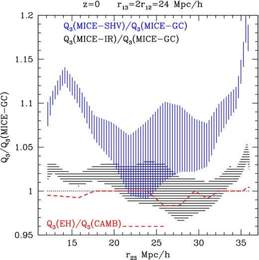
This is similar to Fig. 11 but for smaller scales r13 = 2r12 = 24 Mpc h−1. Here, we show the ratio of the low-resolution results with respect to the one with highest resolution (MICE-GC). Deviations from unity are significant given the errors (shaded regions) and do not seem to arise from small differences in the transfer functions used (dashed lines).
The observed trend of increasing mass-resolution effects as one samples smaller (more non-linear) scales seems consistent with previous analyses of the three-point function on even smaller scales, i.e. ∼1 Mpc h−1 (Fosalba, Pan & Szapudi 2005), where measurements on comparable resolution simulations exhibit more configuration dependence than the halo model predictions (see bottom panels of their Fig. 10).
5.2 Realization effects
In some particular triangular configurations, when we have very large scales r ≃ 80–100 h−1 Mpc but small errors, we can detect some systematic differences that seem to be caused by the power spectrum realization. When using a single simulation, the simulated spectrum is typically slightly different to input transfer at the largest scales because of sampling variance. This is illustrated in Fig. 14, which compares configurations with r12 = r13 = 48 h−1 Mpc in MICE simulations that uses EH and camb transfer functions. On both the largest scales (r23 ≃ 90–100 h−1 Mpc) and intermediate scales (r23 ≃ 40–70 h−1 Mpc) the values of Q3 are significantly different in the two simulations. The differences at intermediate scales can be understood because of the difference in the initial transfer function of the simulations. When we compare the results to the corresponding PT predictions (in the bottom panel), we find no significant deviations (within 3σ errors) between measurements and (tree-level) PT results on this intermediate scales, also indicating that particle resolution does not seem so important for these configurations, given the errors. Note that the errors in MICE-GC and MICE-IR are from Jack-knife (JK) resampling, while the error in MICE-SHV are obtained by dividing the very big box into 27 subsamples.
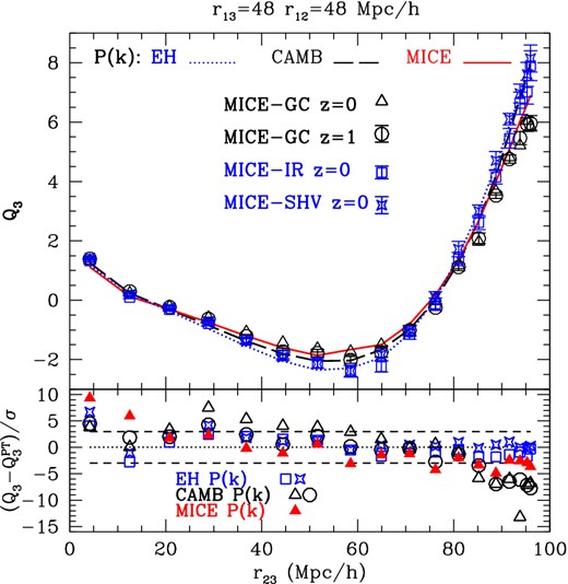
Comparison of Q3(r23) measurements (symbols) for r13 = r12 = 48 h−1 Mpc in different MICE simulations, with predictions (lines) based on the initial transfer function P(k) used in each simulation (EH for IR and SHV, and camb for GC). Measurements in MICE-IR (squares) and MICE-SHV (stars) agree well with predictions from EH transfer function. MICE-GC measurements (triangles and circles) are significantly lower than the camb predictions at the largest scales, but give comparable results at z = 0 and 1. The bottom panel shows the significance of the differences with respect to the corresponding prediction. The MICE-GC result compared to camb (open circles and triangles) show more than 5σ deviations at scales r23 > 90 h−1 Mpc. This discrepancy reduces to 3σ when we use the prediction estimated using the measured MICE-GC P(k) (closed triangles).
On the largest scales, the differences between the EH and camb transfer functions are small (i.e. compare dotted line to dashed line, which lie on top of each other for r23 > 90 h−1 Mpc), but the MICE-GC simulation (circles and triangles) seem significantly lower than the MICE-IR or MICE-SHV results. We find very similar results at other redshifts. The differences are not caused by the binning in the scales defining the sides of the triangles (r12, r13, r23) and the effect does not seem to be caused by resolution (given the agreement within errors with the corresponding predictions at lower scales and the agreement on all scales between MICE-IR and MICE-SHV). These differences seem to originate in sampling variance in the realization of the initial transfer function of the MICE-GC simulation on the smallest k modes.14 This is hinted when comparing the open and closed (red) triangles in the bottom panel. Here, the open triangles compare MICE-GC (z=0) measurements to the camb prediction (which is the input to the MICE-GC simulation), while closed triangles compare the same measurements to the predictions based on the actual measured MICE-GC power spectrum. This is different from the camb predictions because of sampling variance in the MICE-GC realization of the camb transfer function. While deviations with the CAMBP(k) predictions are quite significant (between 5σ and 10σ), deviations with the MICE-GC P(k) predictions are lower (within 3σ). The values at z = 1 (squares) show a similar trend, indicating that this is not just an evolution effect. This figure also illustrates how Q3 does not evolve much with redshift (compare circles, z = 1, and open triangles, z = 0) and that PT predictions are more accurate for intermediate scales than for small or large scales: i.e. it fails more for triangles that are collapsed (see also Bernardeau et al. 2002). As discussed above, the lower resolution simulations (squares and stars) seem to agree better with PT results because of the artificial suppression of non-linearities (i.e. due to poor mass resolution).
Once we use the right shape of the power spectrum, the measurements seem to match predictions within 3σ (dashed lines in bottom panel), although the agreement is even better for triangles that are less collapsed. In general, we do not expect tree-level PT to match the simulations perfectly and some deviations are expected due to higher order (loop) corrections (see Bernardeau et al. 2002).
6 CONCLUSIONS
We have presented one of the largest N-body runs completed to date: the MICE-GC lightcone simulation, containing about 70 billion particles in a 3 Gpc h−1 periodic box. This combination of large volume and fine mass resolution allows us to resolve the growth of structure form the largest (linear) cosmological scales down to very small (tens of kpc) scales, well within the non-linear regime. Therefore, the MICE-GC presents multiple potential applications to study the clustering and lensing properties of dark matter and galaxies that can be confronted with observations from upcoming galaxy surveys.
Furthermore, we have populated haloes with galaxies using a hybrid Halo Occupation Distribution (HOD) and Halo Abundance Matching (HAM) scheme and studied their clustering and lensing properties. Clustering results from the halo and galaxy catalogues are presented in an accompanying paper (Paper II), whereas the all-sky lensing maps and galaxy lensing properties modelled with this new mock are discussed in Paper III. Further details about the galaxy assignment method implemented to build the MICE-GC mock galaxy catalogue will be presented in forthcoming papers (Carretero et al. 2014; Castander et al. 2014).
We make a first public data release of the MICE-GC galaxy mock, MICECAT 1.0, through a dedicated web portal for simulations, hosted by the Port d'Informacio Cientifica (PIC): http://cosmohub.pic.es, where detailed information on the data provided can be found.
In this first paper of the series (Paper I), we have discussed a basic validation and the applications for the dark matter comoving and lightcone outputs, using 2D and 3D statistics. Throughout the paper, we have investigated how mass-resolution effects impact dark matter clustering in the non-linear regime. In other words, we have discussed how much our N-body measurements on small scales might be limited by the particle mass used. Although a proper systematic study based on an ensemble of simulations will be presented elsewhere, we have obtained a series of results and conclusions from the MICE-GC run alone that we summarize below.
The main findings of this paper are as follows.
Using MICE-GC we can measure the BAO pattern in the 3D dark matter power spectrum with high precision. We find very good agreement with RPT predictions at two-loops and k ≲ 0.2–0.3 h Mpc−1, see Fig. 3. There is also a good match comparing to state-of-the-art numerical fits, although we find a slight excess broad-band power (≲ 2 per cent) with respect to the extended Coyote emulator (Heitmann et al. 2014) and the revised Halofit (Takahashi et al. 2012) at z > 0. We note that these differences appear larger than our statistical error bars on those scales (see Figs 3 and 4).
Detailed comparison across redshift evolution and non-linear scales between the power spectrum measured in MICE-GC and recent numerical fits shows that they agree well, but the latter seem to slightly overpredict the power on BAO scales, especially at z > 0 (see Fig. 4). This is more clearly seen beyond BAO scales (k > 0.3 h−1 Mpc) for the recently revised Halofit fitting formula, where the effect reaches 5–8 per cent depending on redshift.
By comparing the 3D power spectrum of MICE-GC to an order of magnitude lower resolution run with the same cosmology, the MICE-IR, we conclude that the change in clustering power produced by mass-resolution effects increase with decreasing scale and grow with redshift. Resolution effects are within 2 per cent for k < 0.2 h Mpc−1 for z < 1, but can be as large as 5 per cent for k ≃ 1 h Mpc−1 and z = 1, as shown in Fig. 5.
We have also produced lightcone outputs of the MICE-GC run, following the approach presented in Fosalba et al. (2008). As shown in Fig. 7, the analysis of angular clustering of the projected dark matter in the lightcone yields consistent qualitative results: the MICE-GC measures a 5 per cent excess power for multipoles ℓ ∼ 103 with respect to the lower resolution run. But this grows to 20–30 per cent excess for multipoles ℓ > 103, which correspond to k ≳ 0.75 at z = 0.5, and k ≳ 0.5 for z = 1 in the Limber or small-angle limit. This confirms that the observed power excess is largely due to mass-resolution effects. Moreover, the impact of such resolution effect is even larger for higher redshift, as shown in Fig. 7. This is consistent with what we found from the 3D power spectrum analysis. Similar trends are found in the angular two-point function, as shown in Fig. 8.
Comparison of angular power spectra with recent numerical fits shows that the MICE-GC measurements show an 5–10 per cent excess relative to Halofit (Smith et al. 2003) in the range 103 < ℓ < 104, and a 5–10 per cent deficit with respect to the revised Halofit by Takahashi et al. (2012).
The modelling of the RSD effects in angular clustering, investigated in Section 4.2, concludes that MICE-GC recovers the Kaiser effect on large scales, i.e. a boost of power of the order of ≃ 3 relative to the real space counterpart. On the other hand, non-linear RSD caused by random motions in virialized dark matter haloes tend to suppress power on small scales relative to 3D clustering in real space. This is only seen in 2D clustering for sufficiently narrow redshift bins, and the amplitude of the effect roughly scales with the inverse of the redshift bin width (see equation 4). In particular, non-linearities in RSD, as seen in the simulation (see Fig. 9) appear at much lower multipoles than those where gravitational growth enters the non-linear regime. We find that ℓNL-RSD ≃ ℓNL-growth/10, and similar results hold for the angular 2PCF, i.e. θNL-growth ≃ θNL-RSD/10 ≃ 10 arcmin.
For the three-point function, we find consistent results with those of the two-point statistics. Higher mass-resolution runs resolve better the small-scale power which tends to flatten out the reduced three-point function, Q3 with respect to PT (tree-level) expectation. This effect seems to get worse at higher redshifts, as shown in Fig. 12. We show how the BAO signal can be detected in Q3, as indicated by measurements by Gaztañaga et al. (2009). On BAO scales errors are quite large and resolution effects are not very significant. On small scales (12–24 h−1 Mpc), Fig. 13 shows how the lower resolution simulations, tend to estimate a more anisotropic three-point function than the higher resolution ones, at the 5 per cent level for MICE-IR and up to 15 per cent for the MICE-SHV run (which has about 100 times larger particle mass than MICE-GC). On intermediate scales, the mass resolution produces differences that are systematic and significant. We have learned here that Q3 is quite sensitive to the actual shape of the power spectrum but this can be degenerate with resolution effects for larger volumes, such as the ones in MICE simulations.
In summary, this new large-volume simulation is shown to describe accurately dark matter clustering statistics in a wide dynamic range. From the linear to the highly non-linear regime of gravitational clustering, thanks to its adequate combination of large-volume and good mass resolution. The resulting galaxy mock MICECAT v1.0, described in the accompanying Papers II and III of this series, is made publicly available with the hope that it will be used as a powerful tool to develop and exploit the high-quality data that is expected from the new generation of astronomical surveys.
We would like to thank Volker Springel for useful discussions regarding gadget-2, Antony Lewis and Ruth Pearson for support with the camb sources code, Eric Hivon for help with healpix and discussions about spherical harmonic analysis, and the Barcelona Supercomputing Center (BSC) support staff, especially David Vicente, for their continued support to develop this Grand Challenge simulation. Special thanks to Santi Serrano for his great help with the MICE website, the simulation visualizations, including Fig. 1 in this paper, and for enlightening discussions that led to the development of the simulations web-portal. We are greatly indebted to Jorge Carretero, Christian Neissner, Davide Piscia, Santi Serrano and Pau Tellada for their development of the CosmoHub web-portal. We acknowledge support from the MareNostrum supercomputer (BSC-CNS, http://www.bsc.es), through grants AECT-2008-1-0009, 2008-2-0011 and 2008-3-0010, 2009-1-0009, 2009-2-0013, 2009-3-0013, and Port d'Informació Científica (http://www.pic.es) where the simulations were ran and stored, respectively, and the use of the gadget-2 code to implement the N-body (http://www.mpa-garching.mpg.de/gadget). Funding for this project was partially provided the European Commission Marie Curie Initial Training Network CosmoComp (PITN-GA-2009 238356), the Spanish Ministerio de Ciencia e Innovacion (MICINN), projects 200850I176, AYA-2009-13936, AYA-2012-39620, AYA-2012-39559, Consolider-Ingenio CSD2007-00060 and research project SGR-1398 from Generalitat de Catalunya. MC acknowledges support from the Ramón y Cajal MICINN programme.
Barcelona Supercomputing Center, http://www.bsc.es.
We restrict the comparison to scales (k ∼ 1 h Mpc−1) where shot-noise in MICE-GC is negligible. In addition, the power spectrum estimation was done using a CIC assignment scheme with a large mesh (kNy = 2 h Mpc−1) which, after correction from the FT of the assignment function, is sufficient to avoid aliasing effects on the scales of interest.
This is discussed in detail in section 6.2 of Paper II.
This variance is not captured by our Q3 JK error bars as it is based on sampling the spatial variations within the one single realization of the camb power spectrum.
