


ABSTRACT
Metal absorption systems are products of star formation. They are believed to be associated with massive star-forming galaxies, which have significantly enriched their surroundings. To test this idea with high column density C iv absorption systems at z ∼ 5.7, we study the projected distribution of galaxies and characterize the environment of C iv systems in two independent quasar lines of sight: J103027.01+052455.0 and J113717.73+354956.9. Using wide-field photometry (∼80 × 60 h−1 comoving Mpc), we select bright (MUV(1350 Å) ≲ −21.0 mag.) Lyman break galaxies (LBGs) at z ∼ 5.7 in a redshift slice Δz ∼ 0.2 and we compare their projected distribution with z ∼ 5.7 narrow-band selected Lyman alpha emitters (LAEs, Δz ∼ 0.08). We find that the C iv systems are located more than 10 h−1 projected comoving Mpc from the main concentrations of LBGs and no candidate is closer than ∼5 h−1 projected comoving Mpc. In contrast, an excess of LAEs – lower mass galaxies – is found on scales of ∼10 h−1 comoving Mpc, suggesting that LAEs are the primary candidates for the source of the C iv systems. Furthermore, the closest object to the system in the field J1030+0524 is a faint LAE at a projected distance of 212 h−1 physical kpc. However, this work cannot rule out undiscovered lower mass galaxies as the origin of these absorption systems. We conclude that, in contrast with lower redshift examples (z ≲ 3.5), strong C iv absorption systems at z ∼ 5.7 trace low-to-intermediate density environments dominated by low-mass galaxies. Moreover, the excess of LAEs associated with high levels of ionizing flux agrees with the idea that faint galaxies dominate the ionizing photon budget at this redshift.
1 INTRODUCTION
There is significant observational evidence that cosmic reionization of hydrogen is largely completed by z ∼ 5.7 (e.g. Ouchi et al. 2010; Kashikawa et al. 2011; Komatsu et al. 2011; Larson et al. 2011; Caruana et al. 2012; Finkelstein et al. 2012b; Zahn et al. 2012; Jensen et al. 2013). Zahn et al. (2012) combined Wilkinson Microwave Anisotropy Probe 7 and South Pole Telescope data to model the duration of the epoch of reionization (EoR) by including the kinetic Sunyaev–Zel'dovich effect in their analysis. They report for the most conservative case that the EoR begins at zEoR < 13.1 and is over by zEoR > 5.8 at the 95 per cent confidence level. Moreover, studies of narrow-band (NB) selected Lyα emitters (LAEs) have found that the normalization of the Lyα luminosity function of LAEs is higher at z ∼ 5.7 than z ∼ 6.5 (e.g. Hu et al. 2010; Ouchi et al. 2010; Clément et al. 2012). Since Lyα is a resonant line, a small amount of neutral hydrogen in the intergalactic medium (IGM) is able to reduce the number of Lyα photons that are transmitted. Therefore, a higher transmission of Lyα photons at z = 5.7 would result from a lower fraction of neutral-to-ionized hydrogen in the IGM than at z ∼ 6.5, suggesting that the main reionization process took place at zEoR ≳ 6. Stark et al. (2010, 2011) reported a decrease in the fraction of Lyman break galaxies (LBGs; Steidel et al. 1996) with Lyα in emission from z = 6 to 3, at fixed luminosity, in line with the observational and theoretical expectation of the evolution of star-forming galaxies over this period. However, several spectroscopic campaigns for the identification of z ≳ 7 LBGs have shown very low numbers of Lyα detections (Fontana et al. 2010; Pentericci et al. 2011; Caruana et al. 2012; Ono et al. 2012; Schenker et al. 2012; Bunker et al. 2013; Treu et al. 2013). This suppression of the Lyα emission could indicate a more neutral IGM at z > 6 (although see Bolton & Haehnelt 2013). Finally, a classic piece of evidence that cosmic reionization was probably complete by z ∼ 6 comes from the Lyα forest in the spectra of high-redshift QSOs. They show several examples of complete Gunn–Peterson troughs (Gunn & Peterson 1965) at z > 6 and an optical depth decreasing with cosmic time (e.g. Becker et al. 2001; Fan et al. 2006; Goto et al. 2011; Mortlock et al. 2011).
Becker, Rauch & Sargent (2007) show that the distribution of optical depths in the Lyα forest is better reproduced by models that account for an inhomogeneous ionizing background and non-uniform IGM temperature, which implies that reionization was certainly not homogeneous nor instantaneous (e.g. Schroeder, Mesinger & Haiman 2013). Moreover, a heterogeneous reionization is also predicted by theoretical studies (e.g. Trac, Cen & Loeb 2008; Choudhury, Haehnelt & Regan 2009; Finlator et al. 2009; Mesinger & Furlanetto 2009; Griffen et al. 2012). Hydrodynamical simulations combined with high-redshift Lyα forest data suggest an extended process of reionization that occurs in a ‘photon-starved’ regime (Bolton & Haehnelt 2007). Semi-numerical simulations have explored the implications of this result on the topology of the reionization process. Choudhury et al. (2009) find a two-stage process starting with an ‘inside-out’ topology in which high-density regions hosting ionizing sources are the first to be ionized. From there, reionization proceeded directly into voids while dense regions which hosted no ionizing sources and had remained neutral to this point were slowly ionized from the outside (‘outside-in’).
After reionization is complete, the relative flux of ionizing radiation that is left over could trace the history of reionization of the large-scale structure. In particular, the scatter in the intensity of the UV background is affected by the distribution of sources of the ionizing field (e.g. Mesinger & Furlanetto 2009) and the evolution on the mean free path of ionizing photons (e.g. Miralda-Escudé 2003; Bolton & Haehnelt 2007; Faucher-Giguère et al. 2008). Mesinger & Furlanetto (2009) compare analytic, semi-numeric and numeric calculations of inhomogeneous flux fields and found a highly variable ionization state predicted to persist after reionization at z = 5–6. For example, if reionization proceeded in a fully inside-out geometry, a highly ionized IGM is expected to exist in regions where the density of matter is higher than the average (e.g. Trac et al. 2008), leading to a possible direct observational test for the challenging question of which regions were the first ones to be permanently ionized.
A highly ionized IGM can be detected through metal absorption systems. A typical signature is the presence of strong triply ionized carbon absorption (C iv, ionization energy = 47.89 eV). In the redshift range 5.3 < z < 6.2, only four C iv absorption systems with column densities |$N_{{\rm {C\,{\small {IV}}}}}$| >1014 cm−2 have been reported from a sample of 13 sightlines towards high-redshift QSOs (Ryan-Weber et al. 2009; Simcoe et al. 2011; D'Odorico et al. 2013). Interestingly, two of them lie at similar redshift (z ∼ 5.72–5.73). One strong C iv absorption system at zabs = 5.7242 in the line of sight towards QSO J1030+0524 (Ryan-Weber et al. 2009; Simcoe et al. 2011) is accompanied by a weaker system at zabs = 5.7428 (Simcoe et al. 2011; D'Odorico et al. 2013). The second example is found at redshift zabs = 5.7383 towards QSO J1137+3549 (Ryan-Weber et al. 2009).
The redshift of these three systems is in co-incidence with an atmospheric transmission window at λ ∼ 8180 Å (zLyα ∼ 5.73) and sets the possibility to search for galaxies in their vicinity using ground-based observations. Conveniently located at z ∼ 5.72–5.73, these three C iv systems provide an opportunity to study the connection between the ionization state of the IGM shortly after the EoR and the population of galaxies in their environment on different scales.
The evolution with time of the comoving mass density of C iv (|$\Omega _{{\rm {C\,{\small {IV}}}}}(z)$|) shows a rapid rise between z ∼ 6 and z ∼ 5 (Becker, Rauch & Sargent 2009; Ryan-Weber et al. 2009; Simcoe et al. 2011). This is unlikely to be solely due to a sharp rise in the metal content of the Universe as the star formation rate (SFR) density is reasonably smooth over this short period of time (e.g. Bouwens et al. 2007; Stark et al. 2009, 2013). More recently, D'Odorico et al. (2013) revisited the evolution of |$\Omega _{{\rm {C\,{\small {IV}}}}}(z)$| and found it to be smoothly rising from z ∼ 6 to z ∼ 1.5, as expected from a progressive accumulation of metals. Nevertheless, they also report that the column density distribution function of C iv is lower at 5.3 < z < 6.2 than 1.5 < z < 5.3, which suggests a change in the number density and/or the physical size of the C iv absorption systems. Furthermore, the evolution of the Si iv/C iv column density ratios towards lower redshift currently suggests a change in the ionization conditions of the absorbing gas at z < 5 (D'Odorico et al. 2013). Therefore, it is possible that the observed evolution of the abundance of high-ionization absorption systems is the result of a change in the ionization balance driven by the evolution of the ionizing UV background after the EoR. If the distribution of sources dominates the ionizing field at that time, then the environment of high-redshift highly ionized absorption systems contains information not only on the origin of the enrichment of the Universe but also on the nature of the ionizing sources.
Recent studies suggest that sub-L* galaxies most likely dominate the ionizing photon budget at z ≳ 6 (Cassata et al. 2011; Dressler et al. 2011; Finkelstein et al. 2012b; Jaacks et al. 2012; Kuhlen & Faucher-Giguère 2012; Ferrara & Loeb 2013; Robertson et al. 2013; Cai et al. 2014; Fontanot et al. 2014). Moreover, many authors have observed an anti-correlation between UV luminosity and the strength of the Lyα emission line, with fainter objects showing larger Lyα equivalent widths (e.g. Shimasaku et al. 2006; Ouchi et al. 2008, 2010; Vanzella et al. 2009), and an anti-correlation between the UV luminosity and the fraction of galaxies with Lyα emission (Stark et al. 2010; Stark, Ellis & Ouchi 2011), with fainter objects being more likely to show Lyα emission. Because at high redshift the UV luminosity of star-forming galaxies correlates with the stellar mass (e.g. González et al. 2011; McLure et al. 2011), the interpretation of these trends suggests that it is possible to use LAEs to preferentially select low-mass galaxies.
The two goals of this work are (a) to identify the galaxies associated with the nearby environment of highly ionized C iv absorption systems shortly after the EoR, and (b) to characterize the matter density distribution at larger scales using galaxies as tracers of the large-scale structure. First, if the change in |$\Omega _{{\rm {C\,{\small {IV}}}}}(z)$| is driven only by the metal content of the IGM, meaning that at z ∼ 5.7 the IGM is simply less enriched, then it is reasonable to expect that strong C iv systems are associated with regions of earlier star formation episodes where the IGM was polluted first and for longer times. This is found at lower redshift, 2 ≲ z ≲ 3 (e.g.: Adelberger et al. 2005b; Steidel et al. 2010), where galaxies in denser environment are more likely to have a strong C iv system within 1 h−1 comoving Mpc. Thus, if the absorbing gas at z ∼ 5.7 is not affected by changes in the IGM ionization state, then we would expect z ∼ 5.7 C iv absorption systems near overdensities of LBGs similar to that found at z ≲ 3. Secondly, if the change in |$\Omega _{{\rm {C\,{\small {IV}}}}}(z)$| results from the evolution in the ionizing flux density background fluctuations, then C iv systems at z ∼ 5.7 would trace regions of high flux density of ionizing radiation. In this case, a simple prediction from an inside-out reionization process is a positive correlation between mass distribution and the ionization level of the IGM. Under this scenario, rare highly ionized strong absorption systems would be expected to reside in dense structures that collapsed earlier and were reionized first. Finally, a third scenario involving the reversal of the topology of reionization is also possible. If young low-mass galaxies forming away from the main overdensities provide a final push for the cosmic reionization, then these will be the regions that, at large scales, will present a higher ionizing flux density that favours the detection of C iv in absorption.
We report that C iv absorption systems are found in low-to-intermediate density environments populated by low-mass galaxies and are not associated with overdensities of massive galaxies, which is in tension with the expectation from a fully inside-out reionization, but in agreement with an outside-in reionization during the last stage of the EoR. This work supports the idea that, although reionization is complete by z ∼ 5.7, the predicted inhomogeneous ionizing flux density of the IGM affects the detection of high-ionization metal absorption systems. In this case, the finding that the immediate environment of highly ionized absorption systems at z ∼ 5.7 is dominated by low-mass galaxies is a new piece of evidence that these galaxies are an important source of ionizing radiation at z ∼ 6.
This paper is organized as follows. Section 2 describes the observations, Section 3 explains the photometric selection of the galaxies for the study, Section 4 presents the colours and magnitudes of the LBG and LAE candidates, Section 5 reports the number density of each sample and Section 6 describes in detail their surface density distribution. The discussion on the origin of the C iv and the reionization of the IGM can be found in Section 7. Finally, a summary of the work and the conclusions are presented in Section 8. Throughout this work, we use AB magnitudes and assume a flat universe with H0 = 70 km s−1 Mpc−1 (h = 0.7), Ωm = 0.3 and Ωλ = 0.7.
2 OBSERVATIONS AND DATA REDUCTION
2.1 Subaru data
This section presents the observational data and the reduction process. This work is based on broad-band and narrow-band photometry obtained with Suprime-Cam (Miyazaki et al. 2002) on the Subaru Telescope. We use broad-band Rc, i′ and z′ filters covering the wavelength range ∼5800–10 000 Å and a custom-made NB filter to detect Lyα in emission at redshift z = 5.71 ± 0.04 (NBC iv, λc = 8162 Å, FWHM = 100 Å). Observations with the NBC iv, Rc and i′ bands were acquired on the nights of 2011 March 07–08 and images in the z′ band were obtained on 2011 31 March and 01 April. We observed two fields centred on QSOs SDSS J103027.01+052455.0 (zem = 6.309, RA = 10h30m27|$_{.}^{\rm{s}}$|01, Dec. = 05°24′55|${^{\prime\prime}_{.}}$|0) and SDSS J113717.73+354956.9 (zem = 6.01, RA = 11h37h17|$_{.}^{\rm{s}}$|73, Dec. = 35°49′56|${^{\prime\prime}_{.}}$|9) (Fan et al. 2006), hereafter J1030+0524 and J1137+3549. The total exposure time of the final images and the full width at half-maximum (FWHM) of the point spread function (PSF) are presented in Table 1. Note that the z′-band images have the best resolution in both cases. These values were measured in science images resulting from the reduction process described next.
Exposure time and PSF of science images.
| Field | Filter | Exposure | PSF |
|---|---|---|---|
| time (min) | (arcsec) | ||
| NBC iv | 240 | 0.79 | |
| Rc | 80 | 0.87 | |
| J1030+0524 | i′ | 90 | 0.81 |
| z′ | 116 | 0.69 | |
| NBC iv | 226 | 1.31 | |
| Rc | 100 | 1.11 | |
| J1137+3549 | i′ | 90 | 1.13 |
| z′ | 114 | 0.67 |
| Field | Filter | Exposure | PSF |
|---|---|---|---|
| time (min) | (arcsec) | ||
| NBC iv | 240 | 0.79 | |
| Rc | 80 | 0.87 | |
| J1030+0524 | i′ | 90 | 0.81 |
| z′ | 116 | 0.69 | |
| NBC iv | 226 | 1.31 | |
| Rc | 100 | 1.11 | |
| J1137+3549 | i′ | 90 | 1.13 |
| z′ | 114 | 0.67 |
The data were processed with the software sdfred2 (Yagi et al. 2002; Ouchi et al. 2004a) designed to reduce Suprime-Cam data. The reduction process includes bias subtraction and overscan, flat-field correction, distortion correction, PSF equalization of different exposures (when needed), masking of bad regions (e.g. satellite tracks and saturated pixels), alignment of all frames and stacking to create the final combined image. Detection and extraction of objects was carried out using the source extraction software SExtractor 2.5.0 (Bertin & Arnouts 1996).
In order to have consistent photometry, first we matched the PSF of the field J1030+0524 to PSF = 0.87 arcsec and the field J1137+3549 to PSF = 1.13 arcsec, which equates to the PSF of the filter with the poorest seeing. The catalogue of broad-band detected objects was obtained running SExtractor in dual mode using the best resolution z′-band image for detection and the PSF-matched images for aperture photometry. The two samples of LBGs analysed in this work (Sections 3.1 and 3.3) are extracted from this catalogue. Similarly, the catalogue of NB selected objects used to identify LAEs (Section 3.4) was obtained running SExtractor in dual mode with the NBC iv image for detection and the PSF-matched images for aperture photometry.
The following SExtractor parameters that regulate the detection of sources were used: DETECT_MINAREA=5, DETECT_THRESHOLD=2.0, ANALYSIS_THRESHOLD=2.0 and DEBLEND_MINCON=0.005. For both detection and measurement images, the corresponding rms-map of the background was converted to a weight-map (WEIGHT = 1/RMS2) and provided to SExtractor using WEIGHT_TYPE=MAP_WEIGHT. Colours were computed from magnitudes measured in a 2.0 arcsec aperture (MAG_APER) in J1030+0524 and a 2.4 arcsec aperture in J1137+3549, and MAG_AUTO was used for the total magnitude of an object. Considering that the z′ filter samples the UV continuum (rest-frame 1350 Å) of galaxies at redshift z ∼ 5.7, the continuum magnitude of an object is measured from the best resolution z′-band image.
2.2 Photometric calibrations
The zero-point magnitude in each broad-band image was tested in each field against point-like sources from the Sloan Digital Sky Survey (SDSS) as both of our fields are covered by the survey. Stars were selected with magnitudes in the range ∼18–22 and cross-matched with a total of 690 (545), 1034 (665) and 576 (385) point sources in the Rc, i′ and z′ bands in the J1030+0524 (J1137+3945) field. The best fit to the Sloan magnitudes was found after applying a 3σ-clipping process. Zero-point magnitudes in the J1030+0524 and J1137+3549 field are Rc zp = 34.57 ± 0.11 and 34.52 ± 0.14, |$i^{\prime }_{\rm zp} = 34.62\pm 0.11$| and 34.50 ± 0.11, |$z^{\prime }_{\rm zp} = 33.52\pm 0.07$| and 33.82 ± 0.09, respectively. Fig. 1 shows the residuals after the zero-point correction of the stars selected from SDSS. Magnitudes in all filters in both fields are in good agreement within ±0.2–0.3 mag with respect to the SDSS magnitudes. Note that the increment in the vertical scatter is due to the increase in the uncertainty in SDSS as we approach its point source limiting magnitude. The zero-point magnitudes for the NBC iv band were derived from photometric standard stars observed the same nights. The stars are GD50 for the field J1030+0524 and HZ44 for the field J1137+3549. The zero-point magnitudes are NBC ivzp = 32.28 (J1030+0524) and NBC ivzp = 32.22 (J1137+3549).
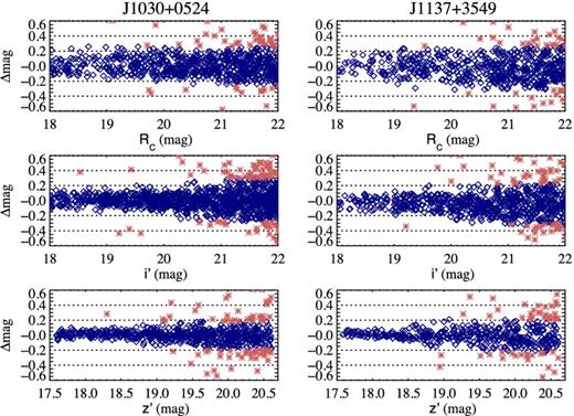
Difference between zero-point-corrected magnitudes and SDSS magnitudes of stars selected from SDSS. From top to bottom, residuals in the Rc-, i′- and z′-band photometry from Suprime-Cam. Diamond points are used to estimate the correction and asterisks represent stars rejected after a 3σ clipping is used in the fitting process.
Galactic extinction from the dust map of Schlegel, Finkbeiner & Davis (1998) is E(B − V) = 0.024 in the field J1030+0524 and 0.018 in the field J1137+3549. We apply a correction of 0.064 (0.048) mag in Rc, 0.050 (0.038) mag in i′ and NBC iv, and 0.035 (0.027) mag in z′ for the field J1030+0524 (J1137+3549).
Aperture corrections in the four bands were estimated from the flux of isolated point sources in 20 apertures from 0.4 arcsec (2.0 pixels) to 6.0 arcsec (29.7 pixels). The measured fluxes level off in a 5.0 arcsec (5.5 arcsec) aperture in the field J1030+0524 (J1137+3549). Therefore, the fractional flux is estimated as the ratio between the flux in the aperture and the flux in a 5.0 arcsec (5.5 arcsec) aperture. We then searched for an aperture with a fractional flux close to 90 per cent in all four bands and find good compromise with a 2.0 arcsec (10 pixels) aperture in the field J1030+0524 and a 2.4 arcsec (12 pixels) aperture in the field J1137+3549. In particular, we find that in the field J1030+0524 the fractional fluxes in an aperture of 2.0 arcsec in the Rc, i′, NBC iv and z′ bands are 86.8, 89.2, 89.1 and 89.6 per cent, respectively, implying aperture corrections of −0.15, −0.12, −0.11 and −0.11 mag. In the same way, in the field J1137+3549 the fractional fluxes in an aperture of 2.4 arcsec are 90.7, 89.9, 75.6 and 94.7 per cent. The corrections for this case are −0.10, −0.11, −0.24 and −0.05 mag.
2.3 Limiting magnitudes
Since the sources of interest are very faint, the magnitude error is dominated by the sky background level. Therefore, the limiting magnitude of each PSF-matched image used for aperture photometry is important to understand the limits of the photometric selection criteria described in Section 3. To estimate the 5σ-limiting magnitude due to the sky level, the background level is measured in 10 000 apertures placed randomly on the sky. The same diameter as for the aperture photometry was used in the measurement images: 2.0 arcsec in the field J1030+0524 and 2.4 arcsec in the field J1137+3549. For z′-band detection images (best PSF), a 2.0 arcsec aperture was used in both fields. Then, the FWHM of a Gaussian fit to the distribution of background counts is used to estimate σ = FWHM/2.354 82 and finally obtain the 5σ-limiting magnitude m5σ = mzp − 2.5log10(5σ). The resulting values and the aperture sizes used on the process are reported in Table 2. Other ways to explore the detection limits of the data are presented and compared to m5σ(z′) in Appendix A.
5σ-limiting magnitude of science images.
| Field | Image | Filter | m5σ | Aperture |
|---|---|---|---|---|
| magnitudes | (arcsec) | |||
| J1030+0524 | Detection | NBC iv | 25.60a | 2.0 |
| Detection | z′ | 25.66a | 2.0 | |
| Measurement | NBC iv | 25.65b | 2.0 | |
| Measurement | Rc | 26.60b | 2.0 | |
| Measurement | i′ | 26.29b | 2.0 | |
| Measurement | z′ | 25.74b | 2.0 | |
| J1137+3549 | Detection | NBC iv | 25.30 | 2.4 |
| Detection | z′ | 25.85a | 2.0 | |
| Measurement | NBC iv | 25.32 | 2.4 | |
| Measurement | Rc | 26.24b | 2.4 | |
| Measurement | i′ | 25.87b | 2.4 | |
| Measurement | z′ | 25.64b | 2.4 |
aBefore PSF matching.
bAfter PSF matching.
3 PHOTOMETRIC CANDIDATES FOR HIGH-REDSHIFT GALAXIES
Broad-band photometry can be used to detect significant features in the observed spectral energy distribution of a galaxy. In particular, the Lyman break technique (Steidel, Pettini & Hamilton 1995; Steidel et al. 1996) has been successfully applied to select high-redshift galaxies as proven by the high fraction of spectroscopic confirmations (e.g. 82 per cent at z ∼ 6, Vanzella et al. 2009; ≥71 per cent at 6 < z < 6.5, Curtis-Lake et al. 2012). However, a galaxy sample will inevitably include contamination from lower redshift objects like reddened elliptical galaxies and Galactic stars. Therefore, defining a criterion to select galaxies based on broad-band colours is a matter of compromise between a clean sample and a complete sample.
In this work, the filters Rc, i′ and z′ on Suprime-Cam were used to sample the rest-frame UV continuum (〈λRest〉 ∼ 1350 Å) and the hydrogen Lyman series (912<λRest <1216 Å) of galaxies at redshift z > 5, as shown in Fig. 2. High-redshift LBGs are identified by the break in their continuum flux at the wavelength corresponding to the limit of the hydrogen Lyman series (λRest ≃ 912 Å) and a significant flux attenuation at wavelengths shorter than Lyman α (λRest ≃ 1216 Å) caused by the presence of neutral hydrogen in the IGM. For example, using similar filters the most common colour selection that aims to identify such features at redshift z ∼ 6 is (i′ − z′) > 1.3, and no detection (e.g.: Rc < 2σ) in a bluer band when available (Bunker et al. 2004; Stanway et al. 2004; Stiavelli et al. 2005; Bouwens et al. 2007; Kim et al. 2009; Vanzella et al. 2009; Stark et al. 2010; Pentericci et al. 2011). We will refer to this criterion as ‘standard’ for z ∼ 6 LBGs or i′-dropout.
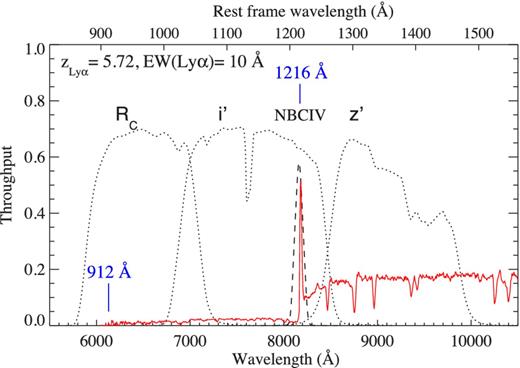
Throughput of filters NBC iv (dashed line), Rc, i′ and z′ (dotted lines) on Suprime-Cam. An LBG template with EW(Lyα) = 10 Å at z = 5.72 is shown in red. The rest-frame wavelength of the Lyman limit and Lyman α is indicated. For z > 5.7, the ‘break’ at Lyα enters the z′ band and can result in a rapid evolution in the (i′ − z′) colour.
The redshift of interest for this work (z ∼ 5.7) falls near the lower end of the redshift distribution probed by the i′-dropout criteria. Therefore, to optimize the selection of galaxies at z ∼ 5.7, it is necessary to understand the limitations of the standard i′-dropout criteria. Furthermore, some authors have noted that a hydrogen Lyman α emission line redshifted to the long-wavelength end of the ‘dropout’ band (i.e. i′ band in this case, see Fig. 2) can influence the colour of a galaxy (e.g. Stanway et al. 2007; Stanway, Bremer & Lehnert 2008). Considering that recent observational evidence suggests that the fraction of galaxies with strong Lyα in emission [Lyα equivalent width EW(Lyα) > 20 Å] is >50 per cent at redshift ∼6 (e.g. Stark et al. 2011; Curtis-Lake et al. 2012), the impact of the equivalent width of the Lyα line on the broad-band colours of LBGs is studied prior to defining an alternative colour selection for z ∼ 5.7 LBGs.
3.1 Selection of z ∼ 5.7 LBGs
This section presents the strategy adopted to select LBGs at z ∼ 5.7 based on broad-band colours. First, we present the template spectra used to explore the colours of the targeted galaxy population using spectrophotometry. Secondly, we discuss each of the explored parameters and the results from the spectrophotometry of the templates. Thirdly, the resulting selection criteria are presented in Section 3.2. Finally, the simulated observations used to define the colour selection criteria are described in Appendix B and the contamination factors are discussed in Appendix C.
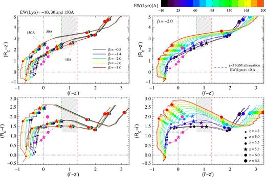
Colour–colour diagrams showing the evolution of LBGs from redshift z = 4.1 to 6.5. The vertical red dashed line indicates the boundary for i′-dropout selection (i′ − z′) = 1.3. The green dot–dashed line indicates the criteria for z ∼ 5 objects: (Rc − i′) > 1.2, (i′ − z′) < 0.7 and (Rc − i′) > (i′ − z′) + 1.0 (Ouchi et al. 2004a). The hashed region shows the window of interest where z ∼ 5.7 LBGs with low EW(Lyα) are found. Left: tracks are colour-coded according to the slope of the UV continuum β, for three templates with EW(Lyα): −10, 30 and 150 Å, respectively. Templates with the same EW and different β are almost indistinguishable from each other, particularly above z ∼ 5. Right: tracks are colour-coded according to the equivalent width of the Lyα line. The slope β was fixed to −2.0. The size of the solid circles indicates the redshift of the template. All models meet the criterion (i′ − z′) > 1.3 for z ≳ 6. The star symbol indicates z = 5.7 and shows that galaxies at z ≲ 5.7 do not meet the i′-dropout standard criteria. The Lyα emission line acts to make galaxies bluer and affects objects at z = 5.7 by moving them away from the hashed region, which, therefore, contains only LBGs with EW(Lyα) ≲ 30 Å. The dashed magenta line shows the colour–colour evolution of a template with EW(Lyα) = 10 Å with the attenuation due to the Lyα forest for objects at z ∼ 3.
3.1.1 Template spectra for target galaxies
This section presents and discusses the template spectra used to compute the spectrophotometry of target galaxies.
Using stellar population synthesis models to simulate the spectrum of a galaxy implies the assumption of intrinsic properties like age, SFR, metallicity, etc. In addition, they typically assume a single stellar population. In this work, we adopt a different approach by using the four composite spectra of LBGs at redshift ∼3 representative of the quartiles of the EW(Lyα) distribution from Shapley et al. (2003) as initial templates for the analysis of the colour–colour diagram of high-redshift galaxies. Referring to the z ∼ 4 composite spectrum of Jones, Stark & Ellis (2012), the changes in LBG spectra have a negligible effect on the broad-band filter colours. Therefore, our results do not depend on any assumption on the intrinsic properties of the galaxies. In other words, the selection criteria introduced in Section 3.2 are based on templates that represent the average properties of a well-studied sample of observed galaxies.
The two spectroscopic features that could influence the UV colours the most are the Lyα line and the UV spectral slope. The reported values in Shapley et al. (2003) are β = −0.73, −0.88, −0.98 and −1.09, and EW(Lyα) = −14.9, −1.1, 11.0 and 52.6 Å for the four templates denoted here as T1, T2, T3 and T4, respectively. Using the templates ‘as they are’ and only accounting for IGM attenuation, we find no significant difference in the redshift evolution of templates T1, T2 and T3 in the colour–colour diagrams (i.e. differences in colour–colour tracks among the templates are smaller than photometric errors). This is not surprising owing to the narrow range of β slopes (−0.73 to −1.0) and Lyα equivalent width (−15 to 11.0 Å) that they cover. The only exception is T4 which departs from the general trend in colour space for redshifts 5.5 < z < 5.9 but this effect is driven by the Lyα emission and is discussed in Section 3.1.3. Thus, it is safe to conclude that no dependence is found with the choice of initial LBG templates. Because the templates represent the four quartiles of the EW(Lyα) distribution of LBGs at z ∼ 3, we use T1 and T2 as templates for LBGs with Lyα in absorption (net EW(Lyα) ≤ 0 Å), T3 as template for LBGs with low Lyα emission (0 < net EW(Lyα) ≤ 30 Å) and T4 as template for LBGs with strong Lyα emission (EW(Lyα) > 30 Å).
3.1.2 UV spectral slopes
Fig. 3 shows the effect of the Lyα emission and the UV spectral slope β in the evolution with redshift of the observed colours of template spectra. The left-hand panels present templates with EW(Lyα) = −10, 30 and 150 Å, colour-coded according to β. At z ≥ 5.5, β is the slope of the continuum that is covered by the z′ band. Thus, it has practically no impact on the colour of the templates and the tracks are almost on top of each other. Moreover, even at z = 5 the smearing effect from different UV spectral slopes is comparable to the photometric errors. Therefore, a single value β = −2.0 is adopted for subsequent analyses because it is the typical value for MUV ≤ −19.0 galaxies at redshift z ∼ 6 (e.g. Bouwens et al. 2012).
3.1.3 Lyα equivalent width
It was noticed in previous works that the colours of an LBG could be significantly affected by the Lyα emission line (e.g. Stanway et al. 2008). The total effect depends on the set of filters, redshift of the source and the equivalent width of the Lyα line. As shown in Fig. 3, using Suprime-Cam filters Rc, i′ and z′, we find that for z ∼ 6 (second to largest circles) all the explored EW(Lyα) values result in (i′ − z′) colours that agree with the standard i′-dropout criteria (i′ − z′) > 1.3 (vertical red dashed line). However, at z ≲ 5.8 galaxies no longer meet the criteria. Furthermore, Lyα emission results in an additional effect on the (i′ − z′) colour. To illustrate the significance of this effect, Fig. 3 shows the position of the templates at z = 5.7 with star symbols. The difference in (i′ − z′) between an LBG with Lyα in absorption (EW(Lyα) < 0 Å) and Lyα in emission (EW(Lyα) > 0 Å) grows with EW(Lyα), reaching Δ(i′ − z′) ∼ 1 mag between EW(Lyα) = −10 and = 150 Å. The result is a region on the colour–colour diagram between the z ∼ 5 and z ∼ 6 LBG selection criteria which is devoid of galaxies with strong Lyα emission (shaded region in Fig. 3). We exploit this effect and develop criteria to select z ∼ 5.7 LBGs with little or no Lyα emission in this region.
In summary, the set of filters used by this work can produce a segregation of LBGs with Lyα in emission and absorption at the redshift of interest z ∼ 5.7. This effect is further explored in Appendix B and the selection criteria to generate a sample of bright LBGs with Lyα mainly in absorption are presented in Section 3.2.
3.1.4 Lyα forest attenuation
Neutral hydrogen absorbs radiation at wavelengths shorter than Lyα. Discrete absorption systems in the line of sight towards a background source produce a forest of narrow absorption lines that is called the Lyα forest. The superposition of such absorption systems can significantly reduce the flux observed at λrest < 1216 Å. Moreover, this attenuation will grow with redshift as a result of the increasing fraction of neutral hydrogen in the IGM and the increasing density of the Universe. This key feature is taken advantage of in the detection of high-redshift galaxies. For example, the magenta dashed line in Fig. 3 corresponds to an LBG with EW(Lyα) = 10 Å in which the average flux decrement (DA) was fixed at the average value at z ∼ 3. When the expected DA is considered (i.e. solid colour-coded tracks), the points at z = 6 and 5 are found in the regions corresponding to the selection for z ∼ 6 LBGs (vertical red dashed line) and for z ∼ 5 LBGs (green dot–dashed lines). Without accounting for the correct DA (i.e. dashed magenta tracks), the points do not meet their respective z ∼ 6 or z ∼ 5 colour selection criteria.
3.2 The selection criteria for z ∼ 5.7 LBGs
NB imaging was designed to detect flux excess from an emission line. As a result, star-forming galaxies without dominant Lyα emission or with Lyα in absorption will be missed by this technique. Therefore, a reliable selection of LBGs from broad-band photometry that includes only objects with low Lyα emission plus objects with Lyα in absorption (or non-LAEs) will produce a valuable sample to compare with NB selected LAEs (see discussion in Section 7.1).
Defining the optimal colour criteria based not only on theoretical colour–colour tracks but also on simulated images of objects allows us to account for many observational uncertainties such as aperture corrections, sky background noise and the choice of parameters for source extraction. Moreover, to quantify the efficiency of a colour selection in a particular set of images, it is necessary to simulate the observation of the targeted objects, in this case high-redshift LBGs. We used our analysis in the previous section to compute magnitudes in the filters Rc, i′ and z′ for templates covering a wide range in EW(Lyα) and a resolution in redshift of Δz = 0.01. The magnitudes are used to generate artificial objects in the science images which are later extracted and reduced as real sources. The results of this exercise provide the basis to define colour selection criteria for z ∼ 5.7 LBGs. The details of our simulated observations and their results are presented in Appendix B, and the possible sources of contamination are reviewed in Appendix C.
Cooke (2009) proposes a method based on broad-band colours of galaxies at z ∼ 3 to select a sample of LBGs with Lyα predominantly in emission and a sample of LBGs with Lyα mainly in absorption and find different environments for each population (Cooke, Omori & Ryan-Weber 2013). In essence, we are applying a similar procedure to higher redshift galaxies and we aim to select LBGs that occupy a narrow redshift range around z ∼ 5.7. In particular, the z ∼ 5.7 LBG selection criteria for this work can be described as a magnitude–colour–colour selection plus a size restriction. The sample meets the following conditions:
z′ ≥ 24,
S/N|$_{z^{\prime }} \ge 5$|,
0.7 ≤ (i′ − z′) ≤ 1.3,
(Rc − z′) ≥ (i′ − z′) + 1.2,
rhl ≤ 0.45 arcsec (or 2.23 pixels),
ISO_AREA_Rc < 22 pixel2, and
0.01 ≤ S/G|$_{z^{\prime }}< 0.9$|,
Several sources are affected by common undesired artefacts of observations. For example, saturated columns and empty columns in the image caused by bright stars can simulate a non-detection in a particular band. These types of effects in Rc or i′ produce incorrectly selected objects. Therefore, after applying the selection criteria, these and other types of ‘bad column’ objects are removed from the sample by visual inspection. Next, we present the selection of z ∼ 6 galaxy candidates, also called i′-dropouts.
3.3 Selection of i′-dropouts
This section describes the criteria adopted to select LBGs at z ∼ 6. The QSO in the field J1137+3549 is at zem = 6.01 and the QSO in J1030+0524 is at zem = 6.309. These redshift values are within the expectations for a sample of i′-dropouts from the spectrophotometry of the LBG templates and the sensitivity of the data. Therefore, a sample of i′-dropout selected LBGs would be more likely associated with the environment of the background QSOs than the C iv systems.
Moreover, Fig. 3 shows that all LBG templates and possible combinations of β and EW(Lyα) reach (i′ − z′) colours redder than 1.3 by z ∼ 6. Thus, we adopted the standard i′-dropout criteria (i′ − z′) > 1.3, plus the additional restrictions described in the previous section, to sample z ∼ 6 LBGs. In particular, i′-dropouts are selected using the following conditions:
z′ ≥ 24,
S/N|$_{z^{\prime }} \ge 5$|,
(i′ − z′) > 1.3,
S/N|$_{R_{c}}< \ 2$|,
rhl ≤ 0.45 arcsec (or 2.23 pixels),
ISO_AREA_Rc < 22 pixel2, and
0.01 ≤ S/G|$_{z^{\prime }} <$| 0.9.
As with the z ∼ 5.7 LBGs sample, individual i′-dropouts are inspected by eye to remove objects that lie in bad columns of the image and are wrongly measured as no detections in the Rc and i′ bands. The final candidates are presented in Tables E3 and E4 (Appendix E). Next, we present the strategy adopted to identify LAEs at redshift z ∼ 5.7.
3.4 Selection of z ∼ 5.7 LAEs
This section presents the selection criteria that define the LAE sample based on NB photometry using the NBC iv filter. The filter detects the Lyα emission of galaxies at redshift z ∼ 5.71 ± 0.04, which traces the more recent star formation episodes in the environment of the C iv absorption systems. The LAE selection is based on the detection of flux excess in the NBC iv band with respect to the i′ band due to Lyα emission. This excess is measured in the colour (i′−NBC iv). Following the criteria defined by Ouchi et al. (2008), and accounting for the small filter difference, the strongest condition of the selection criteria for LAEs is (i′−NBC iv) > 1.335.
Considering the redshift of the target galaxies, the neutral hydrogen in the line of sight produces the same flux decrements at λ ≲ 912 and λ ≲ 1216 that characterize z ∼ 5.7 LBGs (Fig. 2). This feature can be used in the selection by including a condition in the broad-band colours. Although many LAEs drop out the Rc band, the (Rc − i′) colour is commonly used, for example (Rc − i′) > 1.0. However, we have found that some objects with significant flux excess in the NBC iv are not detected in i′. In some of these cases, the alternative colour (Rc − z′) seems to be complementary. Therefore, we defined an alternative condition (Rc − z′) > 1.3. Finally, some objects have significant NBC iv flux (NBC iv >5σ) but are not detected in any of the broad-bands (i.e.: Rc < 1σ, i′ < 1σ and z′ < 1σ). We also included these objects as part of our LAE sample.
Finally, we note that only colour criteria are included in the LAE selection as no additional conditions are applied. The selection criteria are the following:
S/N|$_{{\rm NBC\,{\small {IV}}}} \ge 5$|,
(i′−NBC iv) > 1.335, and
[(Rc − i′) > 1.0] ∪ [(Rc − z′) > 1.3] ∪ [(Rc < 1σ) ∩ (i′ <1σ) ∩ (z′ < 1σ)].
The LAE sample was visually inspected to remove sources in bad columns as for the other two samples of photometric galaxy candidates. Tables E5 and E6 (Appendix E) present the photometry of the LAE candidates in each field.
4 COLOURS AND MAGNITUDES OF z ∼ 5.7 GALAXIES
This section presents colour–colour and colour–magnitude diagrams of the three photometric samples. We find agreement with our expectations from spectrophotometry described in Section 3.1.1 and Appendix B1. We report that LAEs are fainter and have bluer broad-band colours than LBGs selected at similar redshift (z ∼ 5.7). In addition, z ∼ 5.7 LBGs have low NBC iv brightness and only one of them shows evidence of excess in the NBC iv.
It is important to keep in mind that LBGs and LAEs are selected independently. In the first case, photometric catalogues were obtained for z′-band detected sources and the selection is independent of the NBC iv magnitude. In the second case, the catalogues were constructed for sources detected in the NBC iv band and the selection is defined by the excess in this band.
4.1 Broad-band colours
Fig. 4 shows the (i′ − z′) versus (Rc − z′) colour diagram of all sources and highlights the three different samples. The contours contain 50, 90 and 97 per cent of the total number of objects including both fields. The 1σ magnitude limit is assigned to an object when not detected in a particular band (i.e. S/N < 1). For example, many z ∼ 6 i′-dropouts have S/N|$_{R_{c}} < 1$| and S/N|$_{i^{\prime }} < 1$|; hence, they form a diagonal line of red squares in Fig. 4. Objects not detected in two bands will have a constant colour corresponding to the difference in the 1σ magnitude limit of the two bands involved. Due to the limitation of our broad-band photometry, many LAEs are not detected in several broad-bands. For example, LAEs with no detection in Rc and z′ form a horizontal line at (Rc − z′) = 0.86 if the field is J1030+0524 and (Rc − z′) = 0.61 if the field is J1137+3549. The (i′ − z′) colours of these objects are upper limits only determined by their i′ magnitude since the z′ magnitude is set to the 1σ limit. LAEs with no detection in all three broad-bands are overlapping each other in points (0.55, 0.86) if the field is J1030+0524 and (0.22, 0.61) if it is J1137+3549.
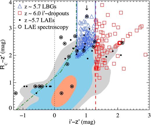
Broad-band (Rc − z′) versus (i′ − z′) colours of the three samples from the two fields of this study: z ∼ 5.7 LBGs (blue triangle), z ∼ 6 i′-dropouts (red squares) and z ∼ 5.7 LAEs (black dots). Open circles indicate LAEs in the spectroscopic sample, which is presented in a forthcoming paper. They all show a single emission line. The arrow indicates the object that is selected by both the z ∼ 5.7 LBG and the LAE criteria. The red dashed vertical line shows the (i′ − z′) = 1.3 boundary for i′-dropouts, the blue solid lines indicate the colour criteria for z ∼ 5.7 LBGs and the green dot–dashed line shows a typical boundary adopted for z ∼ 5 LBGs. The contours correspond to the full catalogue of detections in the z′ band and contain 50, 90 and 97 per cent of the sources in the catalogue.
The most important feature to notice from Fig. 4 is that LAEs have broad-band colours in agreement with our analysis in Section 3.1. First, LAEs detected in both the i′ and z′ bands have colours bluer than the i′-dropout boundary (i′ − z′) = 1.3, as expected due to the presence of the Lyα emission. Secondly, the (i′ − z′) colours of LAEs with S/N|$_{z^{\prime }} < 1$| are upper limits and are consistent with our expectations, i.e. deeper z′-band photometry will result in lower values (bluer colours). Thirdly, although some LAEs occupy the colour space of z ∼ 6 i′-dropouts, they are not selected as i′-dropouts because their z′ magnitudes have S/N|$_{z^{\prime }} \lesssim 2$|. This means that their (i′ − z′) colours have large uncertainties, and it is still possible that their true colour is bluer than our current estimate. Similarly, regarding the LAEs situated in the colour region of z ∼ 5.7 LBGs, all but one have S/N|$_{z^{\prime }} < 5$| and are not included in the LBG sample for this reason. The one exception is the LAE with the highest (Rc − z′) indicated with an arrow in Fig. 4, for which we have spectroscopic confirmation. This object is also selected as a z ∼ 5.7 LBG without using information from the NB and confirms that the selection criteria in Section 3.2 do target bright galaxies in the redshift range of interest. The fact that only one z ∼ 5.7 LBG shows NB excess is evidence that the selection criteria introduced in Section 3.2 certainly avoid most strong emitters.
The LBG samples (z ∼ 5.7 and z ∼ 6) are significantly more sensitive to photometric errors than the LAE sample. The colour criteria for the two samples of LBGs include part of the grey and the blue contours shown in Fig. 4. These contours contain 90 and 97 per cent of the total number of detections in both fields. As a result, the boundaries of the colour criteria are defined in well-populated regions of the colour diagram. This has implications on the effect that photometric errors have in the sample. The reason is that many objects outside the boundaries have colours that, within 1σ error, are consistent with the colour criteria. Similarly, several objects within the colour criteria have photometric errors that may place them outside the colour boundaries. In other words, the level of contamination expected in a sample would increase with the density of objects around the boundaries of the colour selection window. Therefore, the LAE sample is more robust to photometric errors because, as it is shown below, the LAE colour criteria are in a less populated region of the NB colour–colour diagram.
In summary, the few LAEs in the i′-dropout colour region are significantly fainter than the LBG magnitude limit (S/N|$_{z^{\prime }} _cylian_5_o__cylian_2_e__cylian_3_e_) and have large uncertainties in their broad-band colours. LAEs in the colour window of _cylian_2_o_z_cylian_1_e_ ∼ 5.7 LBGs are also too faint to be selected from the _cylian_2_o_z_cylian_1_e_′ band as LBGs. The only exception has S/N_cylian_3_o__cylian_9_o__cylian_10_o_}5$| and it confirms the redshift window aimed at by the z ∼ 5.7 LBG selection criteria introduced in Section 3.2. In general, the distribution of LAEs in the broad-band colour–colour diagram is in agreement with expectations from spectrophotometry of typical LBGs: that strong Lyα emission at z ∼ 5.7 can move the object away from the i′-dropout selection window. Photometric uncertainty affects the number of candidates in the broad-band selected samples because the colour boundaries are densely populated and photometric errors can modify the position of an object in the colour–colour diagram. We include this source of uncertainty in all our results using Monte Carlo simulations of its effect, as explained in Section 5.
4.2 NB colours
The top panels of Fig. 5 present the colour space where LAEs are selected as described in Section 3.4. The green dashed lines show the windows (i′−NBC iv) > 1.335 and (Rc − z′) > 1.3 (left-hand panel), and (i′−NBC iv) > 1.335 and (Rc − i′) > 1.0 (right-hand panel). These boundaries are at >0.3 mag from the grey contour that contains 97 per cent of the sources in both fields. As a result of a very low density of objects near the boundaries, the LAE sample is very stable to photometric uncertainty.
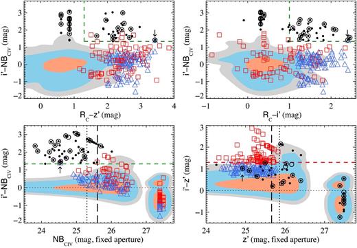
Top: broad-band colours and the excess in the NBC iv: (i′−NBC iv) versus (Rc − z′) (left) and (i′−NBC iv) versus (Rc − i′) (right). Colours, symbols and contours are the same as in Fig. 4. The green dashed lines indicate the boundaries of the LAE colour selection criteria. Bottom left: (i′−NBC iv) versus NBC iv colour–magnitude diagram. Vertical dashed and dotted lines indicate the NBC iv 5σ-limiting magnitudes of field J1030+0524 and field J1137+3549, respectively. Many broad-band selected sources are not detected in the NBC iv band and are assigned the corresponding 1σ magnitude limit (NBC iv1σ ∼ 27.4–27.5 mag). Bottom right: (i′ − z′) versus z′ colour–magnitude diagram. Vertical dashed and dotted lines indicate the z′ 5σ-limiting magnitudes of field J1030+0524 and field J1137+3549, respectively. The horizontal dashed line shows the i′-dropout boundary (i′ − z′) = 1.3. LAEs have fainter broad-band UV magnitude than LBGs.
The condition of S/N|$_{{\rm NBC\,{\small {IV}}}}\ge 5$| implies that all selected objects have NBC iv errors ≤0.198. This means that photometric errors in the NBC iv have negligible impact on the selection of the LAE sample. Moreover, condition (iii) on the broad-band colours of an LAE candidate (Section 3.4) allows the inclusion of objects with no detection in the three broad-bands, which is supported by spectroscopic confirmation of some of these objects. Therefore, contrary to the two LBG samples, photometric uncertainty in the broad-band does not dominate the errors in the LAE samples. Objects not detected in at least two broad-bands form two columns in each panel aligned with (Rc − z′) = 0.86 and 0.61, and (Rc − i′) = 0.31 and 0.39, respectively. Most of them are indeed not detected in the three broad-bands; however, we have spectroscopic detection of an emission line from all the LAEs selected for spectroscopic follow-up (open circles).
We note that five i′-dropouts have (i′−NBC iv) > 1.335. However, because they are not detected in i′ and have S/N|$_{{\rm NBC\,{\small {IV}}}} < 3$|, their (i′−NBC iv) colours have large uncertainties. This is more obvious in the bottom-left panel of Fig. 5 which shows the 5σ detection limit in the NBC iv band with vertical lines, dashed for the field J1030+0524 and dotted for the field J1137+3549. In this figure, we can see how i′-dropouts with significant NBC iv excess are actually not detected in i′ and their (i′−NBC iv) colours are dominated by their faint NBC iv magnitude. Moreover, these objects belong to the field J1137+3549 which has a brighter NBC iv magnitude limit than the field J1030+0524. Finally, the black arrow in Fig. 5 shows the only z ∼ 5.7 LBG that has significant (i′−NBC iv) flux excess, while all the other z ∼ 5.7 LBGs have low NB brightness.
4.3 Colour–magnitude diagram
Several studies of LAEs at different redshifts have found that these galaxies are typically fainter and have average UV colours bluer than LBGs. Our results are in agreement with these findings. The bottom-right panel of Fig. 5 shows that LAEs are dominated by fainter z′ magnitude than the two LBG populations. Although the figure also shows that LAEs populate a region of bluer (i′ − z′) colours, this effect is expected from the presence of a strong Lyα emission.
5 NUMBER DENSITY
5.1 Counts of LBGs
This section presents the sample resulting from the i′-dropout and the z ∼ 5.7 LBG selection criteria. We compare the number of objects per magnitude bin and the total number of objects with expectations from the luminosity function of Bouwens et al. (2007). In general, our results agree with the expected number counts of LBGs at z ∼ 5.7 and i′-dropouts at z ∼ 6.0.
Fig. 6 shows the number of objects detected in the z′ band that meet our selection criteria for z ∼ 5.7 LBGs (Section 3.2). The error bars include Poisson and photometric errors (1σ). To estimate the errors induced by photometric uncertainties, we run the following Monte Carlo simulation. For all the objects in the catalogue of detections produced by SExtractor, the magnitudes in each of the three broad-bands of each object are simulated by randomly selecting a new value from the interval [m − σm,m + σm], where σm is the error in the magnitude m of each detection. In other words: we assume that the real magnitude m of each detection is contained within m ± σm, with uniform probability. Once a new catalogue of detections is created, the selection criteria of Section 3.2 are applied and a new sample of z ∼ 5.7 LBGs is obtained. Then, the number of objects per magnitude bin is recalculated. After 10 000 iterations, the standard deviation of the number counts in each magnitude bin is obtained as the error induced by the uncertainty in the photometry of the sources. Overplotted with red dashed lines are the predicted number of galaxies from equation (D2) (Appendix D) using the Bouwens et al. (2007) luminosity function of z ∼ 6 galaxies. The dotted lines enclose one standard deviation in the three parameters of the Schechter luminosity function (Schechter 1976) reported in Bouwens et al. (2007). Our sample is in general agreement with the currently known luminosity function of high-redshift LBGs.
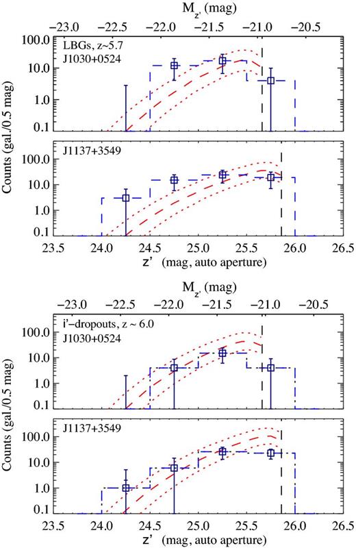
Top: number of LBGs per z′ magnitude bin. The blue dashed histogram corresponds to z ∼ 5.7 LBGs in each field. The error bars include Poisson and photometric errors. The red dashed line shows the prediction from Bouwens et al. (2007) luminosity function and the red dotted lines include the error reported in that work. The vertical black dashed lines indicate the 5σ-limiting magnitude of each field. Bottom: number of i′-dropouts per z′ magnitude bin. The blue dashed histogram corresponds to i′-dropouts (z ∼ 6 LBGs) in each field. As for the plot above, the red lines (dotted and dashed) show the expected number of galaxies ±1σ, according to the Bouwens et al. (2007) luminosity function.
In the field J1030+0524, we select 33 sources as potential z ∼ 5.7 LBGs, and in the J1137+3549 field the number of sources is 61. The expected total number of LBGs from equation (D2) (Appendix D) and the luminosity function of high-redshift LBGs is 18|$^{+22}_{-10}$| in the J1030+0524 field and 39|$^{+44}_{-21}$| in the J1137+3549 field. Although the number of LBG candidates in each field is within the errors of the expected number of galaxies from the z ∼ 6 luminosity function, we note that both samples are larger than the predicted mean number of z ∼ 5.7 LBGs. This is not a surprise since the colour selection window is heavily populated by Galactic cool dwarf stars (Appendix C1) and, despite our attempt to minimize their fraction, the contamination is expected to be higher than that in other LBG colour selection criteria.
The z′ magnitude distribution of i′-dropouts is shown in the bottom panel of Fig. 6. In this case, we select 23 i′-dropouts in the field J1030+0524, where 42|$^{+53}_{-24}$| are expected, and 56 i′-dropouts in the field J1137+3549, where the expectation is 103|$^{+122}_{-55}$|. Although the size of both samples is smaller than the mean predicted number of galaxies for each field, they are within the uncertainty of the luminosity function.
There are several sources of error that can lead to an overprediction in the number of high-redshift galaxies. First, the volume kernel used in equation (D2) is overestimated because we did not account for the area of the sky that is covered by foreground galaxies in the field, which reduce the area of the sky in which high-redshift galaxies can be detected. Secondly, the effect is driven by the faintest magnitude bin (z′ > 25.5, bottom panel of Fig. 6). We are aware that the simulated observations (Appendix B) used to estimate the selection probability function P(m, z) can lead to an overestimation of the number of faint detections because they are based on point-like sources. Using the same detection parameters in SExtractor, at the faintest magnitudes, high-redshift galaxies with relatively more extended light profiles are more likely to be missed than galaxies with the same magnitude but with concentrated light profiles. Therefore, the fainter end of real observations does sample a smaller volume than the one predicted by simulated observations of point-like sources. Thirdly, condition (vii) of the i′-dropout criteria (Section 3.3) that aims to avoid stellar contamination will also remove small galaxies with concentrated light profiles. Considering that bright LBGs are typically more extended than faint LBGs, this condition could also reduce the counts of objects in the faintest magnitude bin. However, the removal of faint ‘suspicious’ sources does not modify our results because we aim to select the UV bright LBGs that trace the most massive haloes.
5.2 Counts of LAEs
We report 45 NB selected LAEs in the field J1030+0524 (total area: 809 arcmin2) and 14 in the field J1137+3549 (total area: 799 arcmin2). Although the samples have different numbers of objects, there is very good agreement between the surface densities of LAEs per 0.5 NBC iv magnitude detected in each field, as shown in Fig. 7.
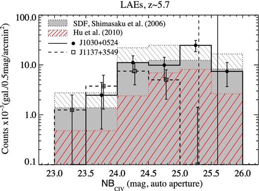
Surface density of LAEs per NBC iv magnitude. Solid line histogram and circles correspond to the field J1030+0524, and dashed line histogram and open squares correspond to the field J1137+3549 (squares have been artificially shifted 0.03 mag). The vertical lines indicate the 5σ-limiting NBC iv magnitude of each field. For comparison, the grey filled histogram corresponds to confirmed z ∼ 5.7 LAEs in SDF from a similar survey area (725 arcmin2) and the red line-filled histogram corresponds to confirmed z ∼ 5.7 LAEs from Hu et al. (2010) from a larger survey area (4168 arcmin2).
The two black line histograms (solid line for J1030+0524 and dashed line for J1137+3549) agree within the error bars, which include Poisson and photometric errors (2σ). The errors are obtained with the procedure described in the previous section. Nevertheless, the Monte Carlo simulation of the photometric errors for NB selected objects allows for an interval [m − 2σm,m + 2σm], from which magnitude values are pulled with uniform probability. As a result, the error bars indicate two times the standard deviation expected from photometric uncertainties. This modification was needed because the LAE selection criteria are not very sensitive to the photometric errors in the broad-band.1 Moreover, the LAE selection requires S/N|$_{{\rm NBC\,{\small {IV}}}}\ge 5$| which makes the excess in the NBC iv to be almost insensitive to the photometric uncertainty. As discussed in Section 4.2, the contour that contains 97 per cent of the sources in Fig. 5 (grey contour) is at >0.3 mag from the colour selection of LAEs. Therefore, hardly any of the 5σ detections from the grey contour could reach the colour criteria in our Monte Carlo experiment, suggesting that the criteria are very stable.
Fig. 7 also shows the observed surface density per NB magnitude (i.e. no completeness correction is applied) of 34 confirmed z ∼ 5.7 LAEs in the Subaru Deep Field (SDF, total area: 725 arcmin2) from Shimasaku et al. (2006, grey filled histogram). The spectroscopic sample from which these objects were obtained contains almost half the SDF LAE photometric sample. Thus, we estimated the predicted surface density assuming the same confirmation fraction for the complete SDF LAE photometric sample. The grey line-filled region shows the possible range of LAE counts in each magnitude bin and suggests that our two samples are in good agreement within the errors with the z ∼ 5.7 LAEs in the SDF.
The red line-filled histogram corresponds to the catalogue of 88 confirmed z ∼ 5.7 LAEs from Hu et al. (2010, total area: 4168 arcmin2). It is slightly below the histograms corresponding to the samples of photometric LAE candidates in the two fields of our study. Such an effect is realistic considering that some level of contamination is present in our photometric samples. Moreover, this catalogue combines seven fields (with some overlap) observed with slightly different exposure times and seeing. Thus, since the surface density is obtained using the total area of the survey, shallower fields will contribute to the total area but not to the fainter end of the distribution in Fig. 7. In addition, two of their fields are in the direction to a massive foreground cluster (z ∼ 0.37) which will affect the ‘effective’ observable area due to a higher number of foreground galaxies and the brightness of the objects due to gravitational lensing. Both of these effects depend on the position in the field of view; thus, the impact on the counts of LAEs is not very clear. Finally, Hu et al. (2010) use a more flexible selection condition in (i′−NB) but almost all the objects were targeted for spectroscopic follow-up. They confirm that a higher (i′−NB) threshold provides a less contaminated sample, but the effect in the total number of confirmations is not significant.
In summary, the surface density per NB magnitude of the photometric samples in the fields of this study is in good agreement with samples from other studies. Next, we present the projected surface density distribution of the galaxies in the environment of the C iv systems (z ∼ 5.7 LBGs and LAEs) and the environment of the background QSOs (z ∼ 6 i′-dropouts).
6 SURFACE DENSITY DISTRIBUTION
In order to characterize the environment of the C iv absorption systems within the large-scale distribution of galaxies in each field, we start with a qualitative analysis of the morphology of the density field traced by the three populations of galaxies. We describe the projected distribution of sources at scales ∼80 × 60 h−1 comoving Mpc and the environment of the C iv systems at a scale of 10 h−1 comoving Mpc. Then, we quantify the surface density of galaxies within 20 h−1 comoving Mpc radius centred in the lines of sight to the C iv systems and we compare our results with expectations from a non-clustered distribution of sources (random distribution).
6.1 z ∼ 5.7 LBGs
In both fields we find that (a) the C iv systems are in a low-density region of LBGs, and (b) the two-dimensional distribution of LBGs shows a clumpy structure.
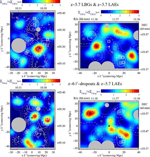
The top panels of Fig. 8 present the position of z ∼ 5.7 LBGs (circles) in comoving Mpc with respect to the C iv lines of sight (white stars). The size of the circles represents the apparent magnitude according to the bins of the histogram in Fig. 6, with smaller circles for fainter objects. The contours indicate constant levels of density contrast quantified by ΣLBG/〈Σ〉LBG, where 〈Σ〉LBG is the mean surface density of LBGs averaged over the size of the field and ΣLBG is the surface density of LBGs obtained using 1 h−1 comoving Mpc bin size and a Gaussian smoothing kernel with FWHM = 10 h−1 comoving Mpc. Dotted contours correspond to underdense regions, dashed contours correspond to mean density regions and solid contours correspond to overdense regions.
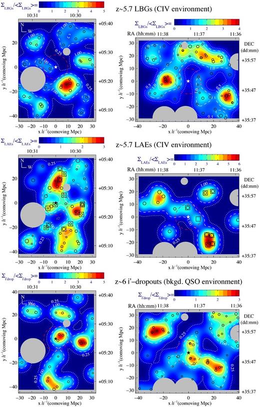
Distribution of z ∼ 5.7 LBGs (top), z ∼ 5.7 LAEs (middle) and z ∼ 6 i′-dropouts (bottom) in the field J1030+0524 (left column) and J1137+3549 (right column). The size of each circle indicates the apparent magnitude bin with larger circles representing brighter magnitudes. The star symbol indicates the line of sight to the C iv systems. Masked areas of the field (bright Galactic stars and edges of the CCD) are shaded grey. The area is colour-coded according to the surface density contrast Σ/〈Σ〉 obtained using 1 h−1 comoving Mpc bin size and a Gaussian smoothing kernel with FWHM of 10 h−1 comoving Mpc. The colour bar of each plot is on the top of each panel. In general, blue colours represent less than the mean surface density of the field and red colours correspond to the highest density of each sample. Yellow and green denote intermediate densities. Dotted contours correspond to underdense regions (Σ/〈Σ〉 < 1), solid contours correspond to overdense regions (Σ/〈Σ〉 > 1) and dashed contours correspond to mean density regions (Σ/〈Σ〉 = 1). The red dashed circle centred on the star symbol has a radius of 10 h−1 comoving Mpc.
We report that, in both fields, the lines of sight to the C iv systems are in regions with a surface density of LBGs lower than the mean of the field, at more than 10 h−1 comoving Mpc from the main concentrations of bright LBGs. The top panels of Fig. 8 show that LBG candidates form ‘islands’ of size ≥10 h−1 comoving Mpc surrounded by large regions where the density is below the mean of the field (blue areas). In both sightlines, a circle of 10 h−1 comoving Mpc radius (red dashed circle) is easily contained between overdensities of LBGs. In other words: at a scale of 10 h−1 comoving Mpc radius, the environment of the C iv looks empty of LBGs in comparison to the rest of the field.
The surface density within a circle of 10 h−1 comoving Mpc radius from the C iv line of sight in the J1030+0524 field (top-left panel) is ΣLBG(10) = 18 ± 16 × 10− 3 gal./arcmin2, which is |$= 0.4^{{+}0.5}_{ - 0.4}$| times the mean surface density of the field 〈Σ〉LBG = 41 ± 5 × 10− 3 gal./arcmin2. In other words: ΣLBG(10) is lower than the mean surface density of the field by a factor of ∼2. The errors include photometric uncertainties and the uncertainty introduced by the masked areas.
In the J1137+3549 field, the surface density within 10 h−1 comoving Mpc radius is ΣLBG(10) = 71 ± 31 × 10− 3 gal./arcmin2 and the total surface density is 〈Σ〉LBG = 76 ± 9 × 10− 3 gal./arcmin2, which results in a density contrast of |$= 0.9^{{+}0.6}_{ - 0.4}$|. Thus, ΣLBG(10)/〈Σ〉LBG ≲ 1 indicates that, at scales of 10 h−1 comoving Mpc, the surface density of LBGs in the environment of the C iv system is in agreement with the mean surface density of the field. At 8 h−1 comoving Mpc radius |$\Sigma _{{\rm LBG}}(8)=28^{{+}37}_{ - 28}{\times }10^{-3}$| gal./arcmin2, which results in a density contrast of |$= 0.4^{{+}0.6}_{ - 0.4}$|, similar to the field J1030+0524 at 10 h−1 comoving Mpc scales.
In the field J1030+0524, the closest LBG brighter than z′ = 25.50 mag is found at 5.1 h−1 comoving Mpc (760.8 h−1 kpc physical, 2.16 arcmin) projected distance from the C iv system line of sight. In the field J1137+3549, the two closest LBGs brighter than z′ = 25.5 are found at ∼8.6 h−1 comoving Mpc (∼1.28 h−1 physical Mpc, ∼3.6 arcmin) projected distance from the line of sight to the C iv system. There are two fainter LBGs (z′ ∼ 25.6-25.7) at slightly closer distances (7.28 and 8.08 h−1 comoving Mpc), but they are also far enough from the C iv to rule out a physical origin.
In summary, the environment of the C iv systems can be described as deficient of bright LBGs with a surface density at a scale of 10 h−1 comoving Mpc that is lower than the mean surface density of LBGs in the entire field of view. Next, we describe the projected distribution of LAEs and discuss the differences with the structure traced by LBGs.
6.2 z ∼ 5.7 LAEs
In both fields we find that (a) the C iv systems are in regions with more LAEs than the average of the field, and (b) LAEs are less clustered than LBGs and surround the concentrations of LBGs.
The distribution of NB selected LAEs is presented in the middle panels of Fig. 8. The size of the circles represents the NBC iv magnitude of the objects. Spectroscopic detections of emission lines are indicated with open squares. Since the spectroscopic data will be presented in a follow-up paper, it is beyond the scope of this work to report our findings from the spectroscopic campaign. Nevertheless, one of the eight spectroscopic confirmations in the field J1137+3549 (Fig. 8, middle-right panel) is not bright enough in the NBC iv band (S/N|$_{{\rm NBC\,{\small {IV}}}} < 5$|) to be in the photometric sample, but is close enough to the C iv line of sight that is considered relevant for the characterization of the environment of the C iv system. Therefore, this object is included in the results presented in this section and Section 6.4.
Contrary to the LBG result, we report a high surface density of LAEs within 10 h−1 comoving Mpc from the C iv systems. In particular, the mean surface density of LAEs in the field J1030+0524 is 〈Σ〉LAE = 56 ± 3 × 10− 3 gal./arcmin2 and the surface density within 10 h−1 comoving Mpc is ΣLAE(10) = 107 ± 4 × 10− 3 gal./arcmin2, which corresponds to a density contrast of ∼1.9 ± 0.2. The errors are small because the uncertainty in the photometry has a negligible impact on the selection of LAEs (Section 4.2) and the very small effect of masked regions is only noticed at scales >10 h−1 comoving Mpc. The three closest LAEs are found at projected distances of 1.43 h−1 comoving Mpc (212 h−1 kpc physical, 0.60 arcmin), 4.70 h−1 comoving Mpc (700 h−1 kpc physical, 1.99 arcmin) and 7.72 h−1 comoving Mpc (1.15 h−1 Mpc physical, 3.27 arcmin). We expand on the closest LAE at 212 h−1 physical kpc in Section 7.2.2.
In the field J1137+3549, the density of LAEs towards the C iv system is also higher than the average of the field. The surface density within 10 h−1 comoving Mpc radius is ΣLAE(10) = 36 × 10− 3 gal./arcmin2, and compared to the mean of field 〈Σ〉LAE = 19 ± 1 × 10− 3 gal./arcmin2 it represents a density contrast of 1.9 ± 0.1. The two closest LAEs are at 7.24 h−1 comoving Mpc (1.08 h−1 Mpc physical, 3.06 arcmin) and 8.02 h−1 comoving Mpc (1.19 h−1 Mpc physical, 3.39 arcmin) from the line of sight to the C iv system.
At scales of ∼80 × 60 h−1 comoving Mpc, LAEs appear to form a filamentary structure, similar to previous findings in other fields from wide-field imaging at similar redshift (e.g. Ouchi et al. 2005a). Furthermore, the particular distribution of LAEs occupies the space between the LBG ‘clumps’. The main concentrations of each population do not share the same position in the field of view which is further enhanced by the fact that the two distributions are in projection. The projected overdensities of LBGs and LAEs (solid line contours, Fig. 8) are in different regions of the field. This pattern is more obvious in the top panels of Fig. 9 that shows the density contrast of both populations using colour-coded contours for z ∼ 5.7 LBGs and line contours for z ∼ 5.7 LAEs, where overdensities of one sample fill the space of underdensities of the other. Interestingly, except for the north-west corner of field J1137+3549, both fields show z ∼ 5.7 LAEs scattered around more compact z ∼ 5.7 LBG groupings. This type of behaviour is observed at z ∼ 3 (Cooke et al. 2013).
Top: density contrast of z ∼ 5.7 LBGs (colour-coded background) and z ∼ 5.7 LAEs (line contours) showing that overdensities of the two samples are not aligned: the solid line contours of both panels are shifted from the yellow and red areas. In general, LAEs (open circles) are found around or between the areas with overdensities of LBGs. The exceptions are one object in the north-west corner of the field J1030+0524 (left-hand panel) and the north-east corner of the field J1137+3549 ( right-hand panel). Bottom: density contrast of z ∼ 6 i′-dropouts (colour-coded background) and z ∼ 5.7 LAEs (line contours). Although the two samples are at different redshifts, the distributions are collapsed in projection and show some agreement and avoidance. The north side and the centre of the field J1030+0524 (left-hand panel) show good agreement between the positions of overdensities of both populations. However, in the south of the field the LAEs are avoiding the positions of the i′-dropouts. In the field J1137+3549 (right-hand panel), agreement is found in the east side and the centre. However, in the west of the field, the overdensities of each sample do not match. Symbol key is as per Fig. 8.
These two galaxy populations likely inhabit different large-scale environments. According to the selection probability function (Appendix D), the depth of the volume sampled by the LBGs (Δz ∼ 0.2) is ∼90 h−1 comoving Mpc, which is similar to the vertical size of the left-hand panels in Fig. 8 (∼80 h−1 comoving Mpc). In addition, the depth of the LAE sample (Δz ∼ 0.08) is ∼36 h−1 comoving Mpc, almost half the vertical size of the field in the left-hand panels. Then, LAEs are contained in the volume sampled by the LBGs. As a result, the projected distribution of the overdensities of each population suggests that, at this redshift, LAEs and LBGs are not evenly distributed (or mixed) in real space.
6.3 z ∼ 6 i′-dropouts
In both fields we find that (a) the line of sight towards the QSO intercepts an overdensity of i′-dropouts, and (b) the projected distribution of i′-dropouts is partially aligned with the distribution of z ∼ 5.7 LAEs but not aligned with the projected distribution of z ∼ 5.7 LBGs.
The distribution of i′-dropouts in the field J1030+0524 (bottom-left panel of Fig. 8) shows three galaxy candidates at projected distances of 2.26 h−1 comoving Mpc (323 h−1 kpc physical, 0.94 arcmin), 4.54 h−1 comoving Mpc (649 h−1 kpc physical, 1.89 arcmin) and 6.60 h−1 comoving Mpc (942 h−1 kpc physical, 2.75 arcmin) from the QSO's line of sight. We find a surface density of i′-dropouts within 10 h−1 comoving Mpc of |$\Sigma _{i^{\prime }{\rm -}\rm {drop}}(10) = 55 \ {\pm } \ 13{\times }10^{-3}$| gal./arcmin2, which is twice the mean surface density averaged over the entire field |$\langle \Sigma \rangle _{i^{\prime }{\rm -} \,\rm {drop}} = 28 \ {\pm } \ 4 {\times }10^{-3}$| gal./arcmin2 (density contrast |$= 2.0^{{+}0.8}_{ - 0.7}$|) and represents an overdensity in the position of the QSO.
A similar overdensity of i′-dropouts is seen in the line of sight towards the QSO in the field J1137+3549. In particular, the two closest i′-dropouts to the C iv line of sight are at projected distances of 4.62 h−1 comoving Mpc (660 h−1 kpc physical, 1.92 arcmin) and 4.84 h−1 comoving Mpc (693 h−1 kpc physical, 2.02 arcmin), with z′ = 25.7 and 25.4, respectively. The next four closest objects are at ∼7.3 h−1 comoving Mpc and have z′ ∼ 25.5. The surface density within 10 h−1 comoving Mpc radius is |$\Sigma _{i^{\prime }{\rm -}\rm {drop}}(10)=146\pm 35 \ {\times } \ 10^{-3}$| gal./arcmin2, which, in agreement with the field J1030+0524, is twice the mean surface density of field |$\langle \Sigma \rangle _{i^{\prime }{\rm -}\rm {drop}} = 70 \ {\pm } \ 8 \ {\times } \ 10^{-3}$| gal./arcmin2 (density contrast |$=2.1^{{+}0.8}_{ - 0.7}$|).
The overdensities of i′-dropouts in the direction to each QSO are very likely associated with the environment of the QSOs, in particular in the field of QSO J113717.73+354956.9 which is at zem = 6.01 (Fan et al. 2006). The i′-dropout criteria applied to the broad-bands used in this work are found to recover LBGs at z ≳ 5.87, which is ≳64.1h−1 comoving Mpc (≳6500 km s−1) from the strong C iv absorption system at zabs = 5.7242 and ≳ 57.8 h−1 comoving Mpc (≳5860 km s−1) from the C iv absorption system at zabs = 5.7383. Thus, our simulated observations described in Appendix B predict that the i′-dropout sample is too far from these C iv systems to be physically associated. Although it is true that photometric errors could introduce objects from lower redshift in the i′-dropout colour selection, this effect is more significant for objects close to the faint end of the selection function, and the three objects within 10 h−1 projected comoving Mpc of the QSO J103027.01+052455.0 (zem = 6.309) are bright sources (z′ ∼ 25.2 mag). Moreover, we have spectroscopic confirmation of one of them at z = 5.973 ± 0.002 (Diaz et al. 2011), originally reported by Stiavelli et al. (2005). In the field J1137+3549, the i′-dropouts in the overdensity towards the QSO are fainter than the field J1030+0524. Hence, photometric errors could explain that some LBGs at redshift z ∼ 5.7 might end up in the i′-dropout sample. However, the large number of candidates in a small projected area implies that this overdensity is extended over a significant fraction of the volume probed by the i′-dropout sample. Therefore, the overdensity very likely covers the environment of the QSO.
Since LBGs are star-forming galaxies, the UV brighter examples are also more massive (González et al. 2011; McLure et al. 2011). Therefore, although the number of objects is low (23 and 56 i′-dropouts in each field, Section 5.1), the sample contains the more luminous objects, which in comparison to the LAEs correspond to older and more massive haloes in the field of view. In the J1030+0524 field, there is good agreement between the positions of the projected overdensities of LAEs and i′-dropouts in the centre and the north half but not in the south half. This is shown in the bottom-left panel of Fig. 9 that compares the surface density of i′-dropouts (colour-coded contours) and LAEs (line contours). Similarly, in the field J1137+3549 the bottom-right panel of Fig. 9 shows good agreement between LAEs and i′-dropouts in the centre and east of the field. However, the west of the field shows the two populations not aligned. Because the contours represent the distribution collapsed in the line-of-sight direction, this behaviour is consistent with the expectation that LBGs trace group overdensities (nodes) and LAEs trace filamentary structures. A filament oriented in the line-of-sight direction will be detected in both samples whereas filaments tangential to the observer will show no counterpart in the sample at higher (or lower) redshift. Moreover, shifted positions of ‘nodes’ in the two distributions correspond to structures with intermediate orientations.
Finally, i′-dropouts are compared to z ∼ 5.7 LBGs (Fig. 10), and their clustering mismatch is more significant. In particular, both fields show that the positions of all the concentrations of galaxies of one sample are shifted from the overdensities of the other sample. The exception is the north-east corner of field J1137+0524 (right-hand panel). This result has important implications for the observed surface density contrast within 10 h−1 comoving Mpc from the line of sight to each QSO. Previously, we showed that while both z ∼ 5.7 LBG samples are underdense in the line of sight towards the background QSO, the i′-dropout samples show the opposite picture with both lines of sight intercepting an overdensity. Therefore, the fact that both fields show the same characteristic density distribution pattern of ‘avoidance’ across the entire field of view strongly suggests that the structure is real.
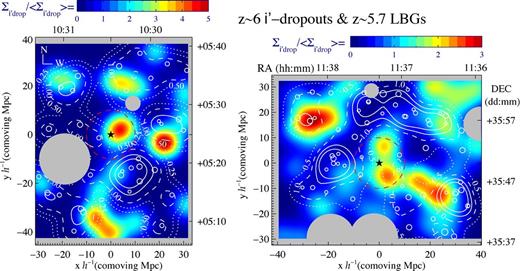
Density contrast of z ∼ 6 i′-dropouts (colour-coded background) and z ∼ 5.7 LBGs (line contours) in the field J1030+0524 (left) and the field J1137+3549 (right). In general, both panels show that overdensities of the two samples are not aligned. Symbol key is as per Fig. 8.
In summary, the overdensities of i′-dropouts are likely associated with the environment of the QSOs in the background, and the mismatch between the distribution of i′-dropout and z ∼ 5.7 LBGs is found across the two fields of view which strengthens the significance of the underdensity of bright z ∼ 5.7 LBGs in the environment of the C iv absorption systems. Moreover, the distribution of LAEs shows partial agreement with i′-dropouts and supports the idea that LAEs trace filamentary structure between nodes of LBGs (e.g. Cooke et al. 2013). In the following section, we compare our results with expectations from a random distribution of sources.
6.4 Expectations from non-clustered sources
This section presents the surface density of each sample of galaxies in the environment of the C iv systems measured as a function of radius and the probability of the observed number of sources assuming a random distribution.
6.4.1 Surface density profiles
Figs 11 and 12 present the surface density profile of the three samples out to ∼20 h−1 comoving Mpc from the lines of sight to the C iv systems in each field. The error bars include Poisson and photometric errors. In order to compare with a non-clustered distribution, 105 random galaxy distributions with the same total surface density of each sample were simulated, from which the surface density was measured radially from the C iv line of sight, after applying the same masks used in the data. The grey shaded areas in Figs 11 and 12 indicate one standard deviation of the radial surface density of the random sample.
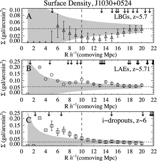
Surface density of galaxies as a function of radius from the line of sight to the C iv systems in the field J1030+0524. The grey area contains ±1 standard deviation from the average of 105 random realizations of galaxy distribution, which were created with the same total surface density of z ∼ 5.7 LBGs (panel A), z ∼ 5.7 LAEs (panel B) and z ∼ 6 i′-dropouts (panel C). The black dotted horizontal line indicates the total surface density of the corresponding sample in the field J1030+0524. The arrows in the top axis of each panel indicate the radial position of objects within 22 h−1 comoving Mpc radius. Panel A shows that the surface density of z ∼ 5.7 LBGs (triangles) in the J1030+0524 field is lower than the mean of the field at most scales out to ∼18 h−1 comoving Mpc. Panel B corresponds to z ∼ 5.7 LAEs (circles) and shows the opposite to z ∼ 5.7 LBGs. With a stronger signal, the number of LAEs is higher than the mean of the field at all scales out to ∼17 h−1 comoving Mpc. In panel C, the surface density of i′-dropouts is higher than the mean of the field at scales ≲ 10 h−1 comoving Mpc. The error bars account for the uncertainty introduced by photometric errors and masked areas. As discussed in Section 4.2, the error bars in panel B are very small because the LAE sample is very stable and the Monte Carlo simulation of the errors very rarely recovers new objects or loses selected LAEs.
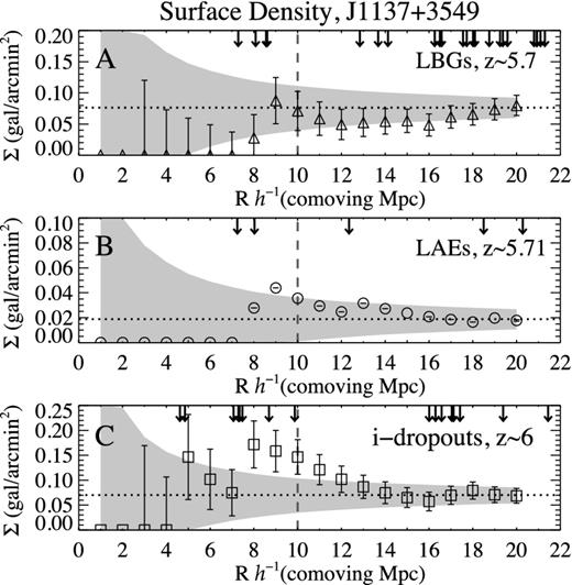
Surface density of galaxies as a function of radius from the line of sight to the C iv system in the field J1137+3549. Symbols and lines are as per Fig. 11. Panel A shows that the surface density of z ∼ 5.7 LBGs is lower than the mean of the field at all scales out to ∼19 h−1 comoving Mpc, in agreement with the field J1030+0524. Panel B shows that the surface density of z ∼ 5.7 LAEs is higher than the mean of the field on scales of ∼8–16 h−1 comoving Mpc, which is similar to our findings in the field J1030+0524 (Fig. 11). In panel C, i′-dropouts are significantly in excess (more than one standard deviation) from the mean of the field, at scales of 8–11 h−1 comoving Mpc and probe the environment of the QSO.
The surface density profile of z ∼ 5.7 LBGs (triangles, top panels) is different from z ∼ 5.7 LAEs (circles, middle panels) in both fields of view. In the first case, the surface density of LBGs in the environment of the C iv is below the total surface density of the corresponding field (the triangles are mainly below the dotted line out to ∼18 h−1 comoving Mpc). This underdensity is more significant in the field J1030+0524 where the largest deficit of LBGs with respect to a non-clustered distribution is at scales of 13 h−1 comoving Mpc. The opposite is observed in the LAE population: in the middle panels of Figs 11 and 12, the circles are above the dotted line out to ∼17 h−1 comoving Mpc. Interestingly, the LAEs show the most significant excess at a scale of 10 h−1 comoving Mpc, close to the scale of maximum deficit of LBGs in the field J1030+0524. Moreover, in Fig. 12, the number of LAEs around the C iv system in the field J1137+3549 is also higher than the total surface density of the field at similar scales (∼10 h−1 comoving Mpc). In summary, both lines of sight intercept regions of the Universe that – at scales of ∼10 h−1 comoving Mpc – have two times more LAEs, and almost half the number of LBGs, than the average in the surrounding ∼80 × 60 h−2 comoving Mpc2.
The i′-dropout samples of the two fields (bottom panels) present similar profiles. First, in the field J1030+0524 (Fig. 11), the QSO line of sight is close to three galaxy candidates and we have spectroscopic confirmation of the closest one. In comparison with the expectation from a uniformly distributed sample (grey shaded area), the surface density is higher than one standard deviation from the mean surface density of i′-dropouts in the field at ≲10 h−1 comoving Mpc scales. At >10 h−1 comoving Mpc, the surface density is in agreement within the errors with the average of the field. Secondly, seven i′-dropouts in the field J1137+3549 (Fig. 12) are within 10 h−1 comoving Mpc from the line of sight to the QSO. Assuming no clustering, the excess in the surface density of i′-dropouts is higher than one standard deviation from the mean of the field at 8–10 h−1 comoving Mpc scales, which was also identified as an excess scale in the LAE samples of both fields.
6.4.2 Probability of the observed number of sources
The 105 random realizations described in Section 6.4.1 were used to estimate the probability of the results under the assumption of no clustering. We calculate the probability, for a random distribution, of the number of galaxies in a circle of 6, 8 and 10 h−1 comoving Mpc radius centred on the C iv lines of sight. We present each field in turn.
Table 3 presents the number of objects detected in each sample at scales of 6, 8 and 10 h−1 comoving Mpc centred on the C iv line of sight, and the probability obtained for a random distribution with the same mean surface density of LBGs, LAEs and i′-dropouts.
Probability of the number of galaxies within a radius of 6, 8 and 10 h−1 comoving Mpc centred on the C iv line of sight in the corresponding field, obtained from 105 random realizations of galaxy distribution (no clustering is assumed) with the same mean surface density of z ∼ 5.7 LBGs, LAEs and i′-dropouts. The errors include photometric errors. For LAEs and i′-dropouts, we present the probability of finding an excess of sources Pr(≥N), except for the case of LAEs in the J1137+3549 field at a radius of 6 h−1 comoving Mpc. For LBGs, we present the probabilities for a deficit of sources Pr(≤N).
| Field | Sample | N6 | P6 | N8 | P8 | N10 | P10 |
|---|---|---|---|---|---|---|---|
| z ∼ 5.7 LAEs | 2 | 0.31a | 3 | 0.32a | 6 | 0.09a | |
| J1030+0524 | z ∼ 5.7 LBGs | 1 ± 0.7 | 0.80b | 1 ± 0.7 | 0.56b | 1 ± 0.9 | 0.32b |
| i′-dropouts | 2 ± 0.5 | 0.10a | 3 ± 0.7 | 0.07a | 3 ± 0.7 | 0.20a | |
| z ∼ 5.7 LAEs | 0 | 0.68b | 1 | 0.50a | 2 | 0.29a | |
| J1137+3549 | z ∼ 5.7 LBGs | 0+1 | 0.21b | |$1^{{+}1.3}_{ - 1}$| | 0.24b | 4 ± 1.8 | 0.57b |
| i′-dropouts | 2 ± 1.2 | 0.40a | 6 ± 1.6 | 0.03a | 8 ± 1.9 | 0.03a |
aPr(≥Nr).
bPr(≤Nr).
Starting with the field J1030+0524, the probability of having three or more LAEs in the field at 8 h−1 comoving Mpc is P8, LAE( ≥ 3) = 0.32. At 10 h−1 comoving Mpc, the probability of having six LAEs or more is P10, LAE( ≥ 6) = 0.09. Thus, we find more LAEs than expected from a random distribution which suggests that the distribution of LAEs is not random and the C iv line of sight intercepts an environment with significant excess of LAEs. This concentration of objects at large scales is not seen in the z ∼ 5.7 LBGs. The random distribution easily predicts a high number of cases with zero or one source for the number of z ∼ 5.7 LBGs. Therefore, z ∼ 5.7 LBGs are found to be consistent with a random distribution. This can also be seen in Fig. 11 where points at 6, 8 and 10 h−1 comoving Mpc are within the shaded regions. In particular at 10 h−1 comoving Mpc, the probability for a random distribution of finding one or less z ∼ 5.7 LBGs is P10, LBG( ≤ 1) = 0.32.
In the field J1137+3549, at 8 and 10 h−1 comoving Mpc scales, z ∼ 5.7 LAEs are consistent with the expectation from no clustering since the probabilities are P8, LAE( ≥ 1) = 0.50 and P10, LAE( ≥ 2) = 0.29. Similarly, the z ∼ 5.7 LBGs are also consistent with a non-clustered sample.
For the i′-dropouts in the field J1030+0524, the overdensity is more significant at scales of 8 h−1 comoving Mpc at which the probability that three objects result from a random distribution is |$P_{8,\,i^{\prime }{\text{-}{\rm drop}}}(\ge 3) = 0.07$|, while the probability at 10 h−1 comoving Mpc radius is |$P_{10,\,i^{\prime }{\text{-}{\rm drop}}}(\ge 3) = 0.20$|. This shows that, around the C iv line of sight, the excess of LAEs and i′-dropouts is peculiar whereas the low density of LBGs could be simply random. Similarly, i′-dropouts in the field J1137+0524 have a probability of six or more sources |$P_{8,\,i^{\prime }{\text{-}{\rm drop}}}(\ge 6) = 0.03$|. Furthermore, at 10 h−1 comoving Mpc radius, the probability of eight or more i′-dropouts is also 0.03.
Our comparison with non-clustered distributions is a good reference point yielding conservative results, since accounting for clustering of sources in our simulated distributions will increase the predicted probability of zero detection, which would enhance the significance of the observed LAE and i′-dropout overdensities. Overall, the results in the field J1137+3549 are in agreement with the field J1030+0524: the excess of i′-dropouts is robustly determined, the deficit of z ∼ 5.7 LBGs is consistent with a random distribution and the overdensity of LAEs is detectable (lower significance in the J1137+3549 field).
7 DISCUSSION
7.1 The impact of the z ∼ 5.7 LBG selection criteria
Many studies on LBGs have found that EW(Lyα) correlates with other galaxy properties (e.g. Shapley et al. 2003; Vanzella et al. 2009; Cooke et al. 2010; Jones et al. 2012). This section discusses the importance of the z ∼ 5.7 LBG selection criteria to directly test a possible correlation between environment and EW(Lyα). First, we summarize the trends previously reported between the UV luminosity and EW(Lyα), to show the differences between the two populations of galaxies presented in this work. The LBG sample comprises only the bright end of the population and is dominated by galaxies with EW(Lyα) ≲ 25 Å. In contrast, our LAE sample includes only galaxies with EW(Lyα) > 20 Å, and is dominated by galaxies with faint UV continuum. Secondly, we review the dependence of UV luminosity and EW(Lyα) with other observables. Finally, we discuss the implications from different clustering properties and the potential dependence between EW(Lyα) and environment.
7.1.1 Two different samples: UV bright LBGs and Lyα bright LAEs
In Section 4.3, we showed that the LAE sample is fainter in the UV (∼1350 Å) than the LBG sample. This result is in agreement with studies of LAEs at z ∼ 5.7 (e.g. Shimasaku et al. 2006) that find emitters with fainter far-UV magnitudes to have stronger Lyα emission. Therefore, a sample of bright LAEs will be dominated by objects with faint UV magnitudes.
Moreover, from a large spectroscopic campaign of z ∼ 3 LBGs, Shapley et al. (2003) reported that the average luminosity in the UV increases with decreasing EW(Lyα). The same trend is observed at higher redshifts (e.g. Stanway et al. 2007; Ouchi et al. 2008; Vanzella et al. 2009; Stark et al. 2010, 2011). As a result, a sample containing the brightest LBGs (MUV < −21.0 mag) will be biased towards low EW(Lyα). Thus, based only on the UV luminosities of the LBGs in our samples, it is reasonable to expect a low fraction of them with Lyα in emission.
Shapley et al. (2003) also reported that LBGs with stronger Lyα emission have bluer continua. In addition, Ouchi et al. (2008) find that LAEs from z = 3.1 to 5.7 have bluer UV continuum colours than dropout LBGs. This is consistent with the picture at z ∼ 3 presented by Cooke (2009), who showed a correlation between the position of an LBG in the colour–magnitude diagram and its EW(Lyα), such that luminous LBGs are dominated by Lyα in absorption with the associated redder UV continua while blue LBGs typically present Lyα in emission. In other words: the LAE population dominates the faint-blue quadrant of the colour–magnitude diagram, while the opposite bright-red quadrant is dominated by LBGs with Lyα in absorption.
At z ∼ 3, Shapley et al. (2003) find weaker low-ionization interstellar absorption and smaller kinematic offset between Lyα and interstellar absorption lines among strong LAEs. At z = 4 and 5, Vanzella et al. (2009) compare the stacked spectra of LBGs with Lyα in absorption and LBGs with Lyα in emission and find stronger interstellar absorption in the composite with Lyα in absorption. Moreover, Vanzella et al. (2009) also compare different morphological parameters (rhl, isophotal area, FHWM and Gini coefficient) of LBGs at 〈z〉 ∼ 3.7 and find that all parameters suggest that LBGs with Lyα in absorption are more extended and diffuse sources than LBGs with Lyα in emission. This Lyα–morphology relationship is also discussed in Cooke et al. (2010). All these results suggest that strong LAEs are younger, less massive and less dusty than strong Lyα absorbers.
Furthermore, following the growth of structure from density fluctuations, more massive objects are expected in denser regions of the Universe. Therefore, it would be expected that two samples of galaxies statistically dominated by different Lyα properties also present different spatial distributions. If LAEs are less massive systems than bright LBGs, then they would be less clustered. As a result, the LAE and LBG samples in this work are complementary tracers of the large-scale structure and the spatial density of these galaxies could be used to characterize different aspects of the large-scale environment.
7.1.2 Distribution of galaxies: is EW(Lyα) an environment indicator?
There is abundant evidence that LBGs are biased tracers of matter, as they inhabit overdense regions of the universe (e.g. Steidel et al. 1998; Ouchi et al. 2004b; Adelberger et al. 2005a; Cooke et al. 2006; Hildebrandt et al. 2009; Bielby et al. 2013). Furthermore, it has been reported that at redshifts z = 3–5.5 more luminous LBGs are more strongly clustered (e.g. Ouchi et al. 2005b; Kashikawa et al. 2006; Lee et al. 2006; Hildebrandt et al. 2009). Recently, Cooke et al. (2013) analysed ∼55 000 LBGs at redshift z ∼ 3 from the Canada–France–Hawaii Telescope Legacy Survey and found that the subpopulation of LBGs with Lyα in absorption (aLBGs) are preferentially in groups, clustered in massive dark matter haloes (∼1013 Mȯ). Interestingly, the subpopulation of LBGs with Lyα in emission (eLBGs) is more evenly spread in space, located in group outskirts and the field. Such an environment–EW(Lyα) connection suggests that the Lyα line could be a statistical indicator of environment. Therefore, in this picture, if the bright LBG population and the LAE population trace different matter density bias, their distributions provide complementary information on the environment at all scales.
Our results cannot rule out an environmental dependence for EW(Lyα). We find UV bright LBGs and Lyα bright LAEs preferentially avoiding each other, with bright LBGs forming ‘clumps’ and LAEs extending and clustering around them. This is in agreement with the expectation that our sample of z ∼ 5.7 LBGs traces the most massive haloes while LAEs inhabit their surrounding areas. As mentioned above, a mismatch between the distribution of LBGs with different EW(Lyα) is inferred at redshift z ∼ 3 by Cooke et al. (2013). If the processes responsible for this effect are already in place at z ∼ 5.7, it is possible that a sample of galaxies selected from a narrower redshift slice will show the ‘shell’-like structure tested in Cooke et al. (2013). Fig. 9 shows that, in both fields, overdensity contours of z ∼ 5.7 LBGs and z ∼ 5.7 LAEs seem to alternate, filling the underdensity regions of each other. We highlight that our selection criteria for z ∼ 5.7 LBGs have the advantage of aiming for a population of galaxies with Lyα preferentially in absorption or low emission (EW(Lyα ≲ 25 Å)) in a cosmic volume (Δz ∼ 0.2) that is a good complement to the LAE sampled volume (Δz ∼ 0.08). Considering that the volumes of the samples are similar, the suggested scenario where galaxies with low EW(Lyα) are more clustered than galaxies with high EW(Lyα) is a simple explanation for our results. Furthermore, it supports the use of LAEs and LBGs as complementary tracers of environment. We will review this topic with follow-up spectroscopy of the samples of this work.
7.2 Environment of C iv systems and the chemical enrichment of the Universe
In this section, we discuss the environment of the C iv systems and the implications from the evolution of the C iv cosmic density |$\Omega _{{\rm {C\,{\small {IV}}}}}(z)$|. First, we review the expectations on the environment of the systems at z ∼ 5.7 from lower redshift observations and find disagreement. We discuss possible scenarios and conclude that background ionizing flux density fluctuations are likely affecting the detection of high-ionization absorption systems. Secondly, the origin of the C iv absorption systems is considered. The predictions from theoretical models that reproduce the evolution of the C iv cosmic density are compared with observational results to conclude that LAEs are the most favourable candidates for the physical origin of the metals. Finally, we comment on previous studies in the J1030+0524 field.
7.2.1 The strongest C iv absorption systems at z ∼ 5.7: implication for the build-up of cosmic metals
The growth of |$\Omega _{{\rm {C\,{\small {IV}}}}}(z)$| with cosmic time has been measured by several authors (Becker et al. 2009; Ryan-Weber et al. 2009; Cooksey et al. 2010; Simcoe et al. 2011; D'Odorico et al. 2013). In this section, we interpret our results as evidence that the ionization state of the IGM plays a role in the observed evolution of |$\Omega _{{\rm {C\,{\small {IV}}}}}(z)$|. We argue that detection of high-ionization systems at z ≥ 5.7 depends on the fluctuations in the background ionizing flux density after the EoR. In this picture, we conclude that higher levels of ionizing flux at z ∼ 5.7 seem to be associated with an excess of LAEs.
Adelberger et al. (2003) analysed the relative spatial distribution of C iv absorption systems and LBGs at redshift 2 ≲ z ≲ 3 and reported significant evidence that strong systems (|$N_{{\rm {C\,{\small {IV}}}}}$| ≥ 1014 cm−2) and LBGs are found in similar parts of the Universe, suggesting that they may be similar objects. Moreover, galaxies in denser environments are more likely to have a C iv system with |$N_{{\rm {C\,{\small {IV}}}}}$| >1013 cm−2 within 1 h−1 comoving Mpc (Adelberger et al. 2005b). Another piece of the puzzle is the significant evidence of galactic outflows in star-forming galaxies at z ≲ 3.5 (e.g. Heckman et al. 2000; Pettini et al. 2002; Shapley et al. 2003; Martin 2005; Rupke, Veilleux & Sanders 2005; Weiner et al. 2009; Dessauges-Zavadsky et al. 2010). In particular, Steidel et al. (2010) report strong evidence for outflowing enriched gas in their LBG sample and find that C iv absorption systems at 〈z〉 ∼ 2.3 are tracing the circumgalactic medium (CGM) of LBGs. These findings show that the surroundings of z ≲ 3 LBGs have been enriched.
If |$\Omega _{{\rm {C\,{\small {IV}}}}}(z)$| is controlled only by the metal content of the IGM, then at z ∼ 5.7 the IGM is simply less enriched. In this case, C iv systems should be found in regions of the IGM that were polluted first, i.e. regions of earlier star formation episodes. Therefore, they would be associated with overdensities of galaxies, as is found at 2 ≲ z ≲ 3 (e.g.: Adelberger et al. 2005b). Similarly, if C iv absorption systems trace the CGM of LBGs, the evolution of |$\Omega _{{\rm {C\,{\small {IV}}}}}(z)$| would simply reflect an increase with cosmic time in the number of haloes hosting strong C iv systems. In this case, for z ∼ 5.7 C iv absorption systems, we still expect a similar environment as found at z ≲ 3.5.
However, in this work we trace back the earliest absorption systems known to date in two lines of sight and find them removed from the main overdensities. The strong C iv absorption systems at z ∼ 5.7 studied here are not found in overdense regions of bright and massive LBGs (L > L*), but in rather underdense regions of the large-scale distribution of z ∼ 5.7 LBGs (top panels of Fig. 8). In the fields J1030+0524 and J1137+3549, the C iv absorption systems are distant (>10 h−1 projected comoving Mpc) from the main concentrations of LBGs. Thus, the high column density C iv systems are not found associated with the earliest star-forming regions.
Furthermore, we report a significant excess of LAEs within 10 h−1 projected comoving Mpc from the C iv absorption systems at z ∼ 5.7 in both fields of view (higher in the field J1030+0524). This result completes the picture that C iv absorption systems are tracing different environments at z ≤ 3.5 and z ∼ 5.7. This is in agreement with D'Odorico et al. (2013) who find that C iv systems at z ∼ 5.7 are better explained by gas with an overdensity of δ ∼ 10 whereas C iv systems at z ∼ 3 are better explained by gas with δ ∼ 100. Moreover, we propose that such a density contrast is linked to larger scales: 8–10 h−1 comoving Mpc. Considering that the presence of C iv is determined not only by the amount of carbon but also by the ionization condition of the gas, our results suggest that the detection of C iv systems, and therefore the rise in |$\Omega _{{\rm {C\,{\small {IV}}}}}$| with cosmic time, is likely affected by a heterogeneous ionizing flux density distribution left over from cosmic reionization. Therefore, whether the ionizing flux is dominated by local sources or the large-scale distribution of ionizing sources, if the ionizing flux density fluctuations have survived at least to z ∼ 5.7, we conclude that higher levels of ionizing flux seem to be associated with excess of LAEs.
Finally, considering that in both fields the closest LBG is at more than 5 h−1 comoving Mpc of the C iv system, our results also imply that the progenitors of strong C iv systems at z ∼ 5.7 are not bright and massive LBGs. We expand the discussion on the origin of the metal absorption systems in Section 7.2.3.
7.2.2 The closest galaxy to a z ∼ 5.7 C iv system
We report one galaxy candidate close enough to the J1030+0524 C iv line of sight to consider the possibility of a direct causal connection through active outflows. The object is a faint LAE selected candidate with NBC iv = 25.11 ± 0.15 mag, barely detected in z′ (z′ = 25.89 ± 0.52 mag, MUV ∼ −20.48) and non-detected in Rc and i′. The object lies at 0.60 arcmin from the sightline towards QSO J1030+0524. Thus, if the object is confirmed to be a z ∼ 5.72 galaxy, it will be at 212 h−1 physical kpc from the C iv system. However, the line of sight to J1030+0524 contains two C iv systems at z ∼ 5.72–5.74 and opens a window to explore the origin of the high-redshift enrichment in better detail. Precise spectroscopic redshift measurements will be required to confirm the association of this LAE with any of the two absorption systems. Spectroscopic data of the object have been obtained with deimos on the Keck Telescope and will be presented in a forthcoming paper.
7.2.3 The origin of z ∼ 5.7 C iv systems
It is well recognized that feedback from galactic winds plays a fundamental role setting the properties of metal absorption systems in the IGM (e.g. Oppenheimer & Davé 2006, 2008; Martin et al. 2010; Cen & Chisari 2011; Tescari et al. 2011), and is important for galaxy evolution (e.g. Martin 2005, 2006; Rupke et al. 2005; Steidel et al. 2010; Bradshaw et al. 2013). This is why we are interested in the properties of the galaxies near the C iv systems. In this section, we present LAEs as the most likely physical origin of strong C iv absorption at this redshift. We review the theoretical expectations and observational results that suggest this scenario, and we present our results as direct evidence to support it.
The evolution of the comoving density of C iv ions in the IGM is only well reproduced by models that include outflows from star-forming galaxies. Oppenheimer, Davé & Finlator (2009) find that C iv at z = 5–6 is a good indicator of metals in the IGM and not gas in galaxies. They predict that strong C iv systems are ionized by the galaxy that produced the enrichment, which would have rest-frame UV magnitudes ≥−18.9 (1350 Å) and stellar masses of 107–108 Mȯ. Current measurements of the stellar mass of LAEs are at the upper end of this range. For example, Gawiser et al. (2006) reported mean stellar masses of 5 × 10⁸h− 2 Mȯ in LAEs at z = 3.1. More recently, Lidman et al. (2012) estimated stellar masses of 108–109h− 2 Mȯ for four of the five bright LAEs at z ∼ 5.7 they analysed.
When considering dark matter haloes, Porciani & Madau (2005) predicted that galaxies in haloes of ∼108–1010 Mȯ at z ∼ 6 could have produced large bubbles of metals that evolve into the environment of z ∼ 3 LBGs. Interestingly, Ouchi et al. (2010) estimated that LAEs at z = 5.7 and 6.6 lie in dark matter haloes of 1010–1011 Mȯ. Moreover, this result holds for LAEs at z = 3.1–5.7. Therefore, faint LAEs are the best candidates for the galaxies responsible for the enrichment of the IGM at z ≥ 6. This idea is supported by the excess of LAEs around the C iv systems in the two fields of view of this study.
Simulations also predict that at redshift z ∼ 6 there should be a closer connection between C iv absorption systems and their parent galaxy as the gas would be in their first journey out of the galaxy (Oppenheimer et al. 2009). Although the LBG sample seems to be too distant to be associated with the C iv systems, in Section 7.2.2 we report an NB selected LAE as the closest galaxy candidate to a C iv system at z ∼ 5.7. This particular example in the field J1030+0524 at ∼212 h−1 projected physical kpc from the line of sight to the C iv is in very good agreement with expectations from cosmological simulations.
In conclusion, our results suggest that the origin of the C iv absorption systems at z ∼ 5.7 is more likely associated with a low-mass LAE type of galaxy than a massive LBG type of galaxy. This argument is strengthened by, first, that the best candidate for a galactic outflow–absorption system causal connection is a faint LAE at 212 h−1 physical kpc in the field J1030+0524 that awaits spectroscopic confirmation, and second, the tentative detection of a C iv absorption system at z = 5.9757 reported by D'Odorico et al. (2013) which is at Δv ∼ 110 ± 85 km s−1 and 325 h−1 physical kpc transversal from the i′-dropout with strong Lyα emission J103024.08+052420.41, at z ≃ 5.973 ± 0.002 (Stiavelli et al. 2005; Diaz et al. 2011). However, the possibility that undetected low-mass young galaxies are responsible for the enrichment of the IGM cannot be ruled out.
7.2.4 Previous environmental studies in the field J1030+0524
Some evidence of a possible overdensity of galaxies in the direction to the QSO SDSS J1030+0524 has been provided by Stiavelli et al. (2005). This result was later confirmed by Kim et al. (2009) based on an excess of galaxies photometrically classified as i′-dropouts (i.e. with i775 − z850 > 1.3), and hence potentially located at z ≳ 5.5. They used the Advanced Camera for Surveys (ACS) on the Hubble Space Telescope as part of a large study of i′-dropouts around five QSOs at z ∼ 6. In particular, 14 ± 4 i-dropouts were found in the field of J1030+0524, compared with 8 ± 3 expected from a random distribution of galaxies at this redshift (Giavalisco et al. 2004).
In this study, we analyse the same field at significantly larger scales, we use an independent method to quantify the density contrast in the field and, although the current photometry is ground based (seeing limited), we include information from a bluer band (Rc) which was not available to previous studies. We find an overdensity of i′-dropouts relative to the projected surface density averaged over scales of ∼80 × 60 h−1 comoving Mpc, in agreement with previous studies.
More recently, Diaz et al. (2011) analysed the spectra of a small sample of three objects in the field J1030+3549 selected as i′-dropouts in Stiavelli et al. (2005). In particular, Diaz et al. (2011) reported positive detection of a spectroscopic feature that at the rest wavelength of the Lyα line would position the objects at zT1 = 5.973, zT2 = 5.676 and zT3 = 5.719 (Targets 1, 2 and 3 of Diaz et al. 2011). However, our z ∼ 5.7 LBG selection does not recover them. Although in our current study the photometry of Targets 1 and 2 is contaminated by a close object, both targets are detected with S/N|$_{z^{\prime }}\ge 5$| and the measured (i′ − z′) colours are in agreement with the values reported in Diaz et al. (2011). Moreover, Target 1 (zT1 = 5.973) has colours expected for z ∼ 6 LBGs and is part of the i′-dropout sample, and Target 2 (zT2 = 5.676) has colours close to the z ∼ 5.7 LBG criteria. Finally, Target 3 is only detected with S/N|$_{z^{\prime }} \sim 2$| and has bluer colours than reported by Diaz et al. (2011). More importantly, we have a 4σ detection in the Rc band (Rc = 26.6 ± 0.3) which implies that, contrary to the other two objects, Target 3 is more likely a low-redshift object than a high-redshift LBG. We also note this object lies very close to the edge of the ACS CCD camera, which can affect the photometry estimated from ACS data. New spectroscopic data have been acquired and the nature of these objects will be reviewed in a future work.
7.3 The IGM and the sources of cosmic reionization
Metal absorption systems provide information of the IGM that could be used to test the topology of reionization. Regardless of whether the C iv systems are IGM or CGM, if the change in |$\Omega _{{\rm {C\,{\small {IV}}}}}(z)$| is the result of ionizing flux density fluctuations, then C iv systems close to the EoR trace regions of high flux density of ionizing radiation. In this case, a simple prediction from an inside-out reionization is a positive correlation between mass distribution and the ionization level of the IGM. Under this scenario, rare high-ionization strong absorption systems would be expected to reside in dense structures that collapsed earlier and were reionized first. However, we do not find that C iv systems are associated with overdensities of massive galaxies.
Young massive stars provide the ionizing flux that caused reionization. This means that the generation of stars that started the process is not the same that finished it. Under this scenario, it is more natural to expect the ionization conditions that allow the detection of strong C iv in regions of more recent star formation. Indeed, our results support a connection between C iv absorption systems and recent star formation at z ∼ 5.7. Moreover, the association with an excess of LAEs favours dark matter haloes of M ≲ 109–1010 Mȯ as progenitors of the C iv systems, consistent with predictions from simulations (e.g. Oppenheimer et al. 2009). As a result, young haloes in intermediate-density regions at z ∼ 5.7 could host the ionization conditions found in overdensities at z ∼ 2–3.
Finally, there is general agreement that fainter galaxies (sub-L*) dominate the ionizing photon budget. In particular at redshift z ∼ 6, Finkelstein et al. (2012b) report that the contribution from galaxies with L > L* to the total specific UV luminosity density is almost the same as galaxies with 0.2L* < L < 0.5L*. In addition, it has been found that LAEs are statistically fainter and less massive than LBGs, which makes them good candidates for sources of ionizing radiation. For example, current evidence suggests that the contribution of LAEs to the ionizing photon budget increases with fainter magnitudes (e.g. Cassata et al. 2011; Kashikawa et al. 2011). Our results suggest a connection between highly ionized IGM and LAEs, which is easily explained if LAEs provide a larger amount of ionizing radiation than UV brighter/more massive LBGs. Therefore, our result is in good agreement with current findings that sub-L* galaxies play a central role in the reionization of the Universe, at least at the final stages of the EoR.
In summary, this work supports the idea that UV faint galaxies are the key to the reionization of the Universe, and is in agreement with an inversion in the topology of cosmic reionization, meaning that in the latest stages of the EoR, the ionizing flux density was higher in lower density environments. Hence, the simplest picture for the environment of the strong C iv absorptions at the highest redshift is a ‘filamentary’ structure populated by low-mass haloes rather than an early overdensity.
8 SUMMARY AND CONCLUSIONS
This is a study of the environment of high column density C iv systems (|$N_{{\rm {C\,{\small {IV}}}}}$| > 1014 cm−2) at z ∼ 5.72–5.74, in the fields J1030+0524 and J1137+3549. Using wide-field photometry in the Rc, i′ and z′ bands, and an NB filter NBC iv, we select LBGs using broad-band colours, and LAEs using NB excess and colours. Our results and conclusions are summarized as follows.
We find the selection criteria for LAEs to be reliable and stable within the photometric uncertainty. We confirm that strong Lyα emission can affect the broad-band colours of the LBG population at the redshift of interest.
We have tested a selection criterion based on broad-band colours that aims for a sample statistically dominated by bright star-forming galaxies with EW(Lyα) ≲ 25 Å (see Section 3), in a redshift slice Δz ∼ 0.2. This z ∼ 5.7 LBG selection criterion is predicted to be more effective at selecting galaxies at the redshift of the C iv systems than the z ∼ 6 i′-dropout criteria. In general, the number of objects detected is consistent with expectations from the z ∼ 6 luminosity function (Section 5).
We compare the projected distribution of LBGs (Δz ∼ 0.2) with NB selected LAEs (Δz ∼ 0.08). A direct comparison of the clustering of the sources is possible thanks to the narrow volume that is sampled. In both fields of view, we find bright UV LBGs in clustered associations and LAEs distributed in the surrounding areas. The structure detected in the distribution of galaxies is consistent, although not definite, with a possible dependence of the EW(Lyα) with environment.
The local environment of C iv absorption systems in the fields J1030+0524 and J1137+3549 presents an excess of LAEs and a deficit of z ∼ 5.7 LBGs per arcmin2 on several scales. In the field J1137+3549, LAEs are low in number but the surface density at a scale of 10 h−1 comoving Mpc is higher than the mean of the field.
i′-dropouts are found in excess towards both QSO lines of sight and are likely related to the background (z ≳ 6) QSO environment instead of the foreground (z ∼ 5.72–5.74) absorption systems of interest. This is in agreement with the expectation that QSOs inhabit massive haloes in the centre of large-scale overdensities and that large-scale overdensities can be traced by LBGs.
Our results suggest that strong C iv absorption systems at the end of the EoR are not related to overdensities of bright and massive (L > L*) LBGs with low or no Lyα emission. Therefore, the environment of strong z ∼ 5.7 C iv systems is different to the examples at lower redshift (z ≤ 3.5). Instead, C iv absorption systems are found in regions dominated by LAEs, which are younger (recent star formation), fainter and lower mass systems than LBGs. This would imply that z ∼ 5.7 C iv systems trace low-to-intermediate density environments and are distant from the oldest star-forming regions of each field.
We report one LAE that lies at ∼212 h−1 physical kpc from the line of sight in the J1030+0524 field. The close proximity suggests that the faint galaxy is the progenitor of one of the two C iv systems in this sightline. This result supports the idea that LAEs are the most favourable candidates for the physical origin of the C iv systems at z ∼ 5.7. Spectroscopic redshift determination is required to test a galaxy–absorption system connection and we will address this topic in more detail in a forthcoming paper.
The results support the idea that the detection of high-ionization absorption systems after the EoR depends on the fluctuations of the ionizing flux density. In this case, the excess of LAEs found in the field J1030+0524 is related to high levels of ionizing flux that allow the detection of C iv. This result implies that faint galaxies are important sources of ionizing radiation, in agreement with many other findings in the literature that propose that faint galaxies are the primary sources driving the end of cosmic hydrogen reionization.
More work on the environment of metal absorption lines in the EoR is needed. Recently, O i absorption systems have been proposed as probes of the physical state of neutral filamentary overdensities in the later stages of the EoR (Keating et al. 2014). If this is the case, at z ≥ 5.7 strong C iv absorption systems with no low-ionization metal lines are the complement to O i absorption systems. It could be possible to combine low-ionization and high-ionization metal absorption lines to study the EoR, because O i are expected to trace the haloes of the galaxies that produced the cosmic reionization (e.g. Finlator et al. 2013), whereas C iv are likely tracing diffuse recently ionized IGM.
ACKNOWLEDGEMENTS
We are grateful to the staff of the Subaru Telescope for their help with the observations. We thank the referee for her/his constructive comments. Many thanks to Greg Poole and Vincenzo Pota for their valuable comments that helped to improve the presentation of this work. CGD acknowledges the support of the funds by the Victorian Government. YK acknowledges the support from the Japan Society for the Promotion of Science (JSPS) through JSPS research fellowships for young scientists. ERW acknowledges the support of Australian Research Council grant DP1095600. JC acknowledges support from Australian Research Council grant FT130101219. Support for this work was provided by NASA through awards, RSA1345996 and RSA1367870, issued by JPL/Caltech.
Based on data collected at Subaru Telescope, which is operated by the National Astronomical Observatory of Japan.
The reason is that many objects are not detected in at least one broad-band and are set to the 1σ limit, which means that their colours depend on one band only. The Monte Carlo simulation of the photometric errors does not randomize the magnitude in the band where the object is not detected. In other words, if a source is not detected in one band, the magnitude assigned is the 1σ limit in every random realization.
REFERENCES
APPENDIX A: DETECTION LIMITS
One approach to estimate the 5σ-limiting magnitude is by searching for the faintest object detected with S/N = 5, which is a 5σ detection. This is equivalent to searching for the faintest point source with an error of 0.198 mag. Fig. A1 shows the z′-band magnitude of each detected source plotted against the corresponding magnitude error. The grey area contains more than 20 objects per bin, the dark grey area contains more than 100 objects per bin and the blue area contains more than 250 objects per bin. Point sources are plotted as black points and detections in the negative image obtained by multiplying the original science image by −1 are plotted as red squares. The horizontal line indicates an error of 0.198 mag. We find that the faintest point source in the J1030+0524 field with a magnitude error close to 0.198 mag has a magnitude z′ = 25.79 mag and a magnitude z′ = 26.01 mag in the J1137+3549 field. They both are in agreement with our previous estimation of the 5σ-limiting magnitude using random apertures (Table 2) which are indicated by the vertical lines.
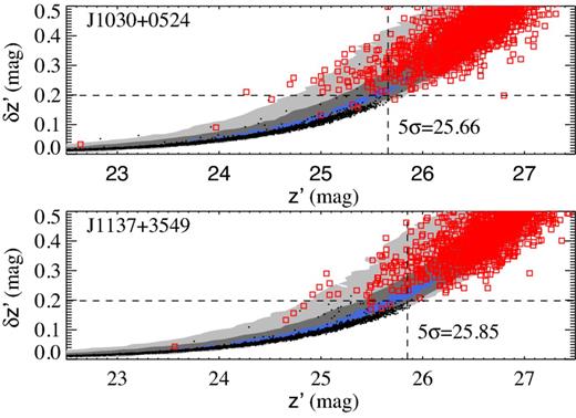
Magnitude–error relation from the z′ band in the fields J1030+0524 (top) and J1137+3549 (bottom). The grey, dark grey and blue contours indicate more than 20, 100 and 250 sources, respectively. Black dots denote point sources and red squares show detections in the negative image. The horizontal dotted line indicates the error of a 5σ detection, i.e. 0.198 mag, and the vertical dotted line indicates the 5σ limit in Table 2, showing that an error-limited sample is cleaner than a magnitude-limited sample.
The histogram of magnitudes provides another rough estimate of the limiting magnitude from the turning point in which the number of objects starts to decrease. Fig. A2 shows the histogram of z′-band magnitudes in the fields of interest. The 5σ limit seems to be in the range 25.8–26.0 mag for the field J1030+0524 and in the range 26.0–26.2 mag for the field J1137+3549, which is equivalent to or slightly fainter than our previous estimates (Fig. A2, vertical dotted line). Also plotted in Fig. A2 is the histogram of magnitudes obtained from the corresponding negative image (dashed line). Since the median background per exposure was subtracted during the reduction to bring the sky level to zero, every detection in the negative image results from fluctuations in the background counts or from bad pixels. Therefore, the number of detections in negative images provides a true measurement of the number of false-positive detections in the original images. The bottom plot in Fig. A2 presents the fraction of false-positive detections obtained as the ratio between the number of detections in the original image and the number of detections in the negative image, per magnitude bin. The horizontal line shows that in both cases the fraction of false detection is less than 1 per cent for magnitudes brighter than m5σ (vertical line). The contamination from false-positive detections is addressed in Appendix C.
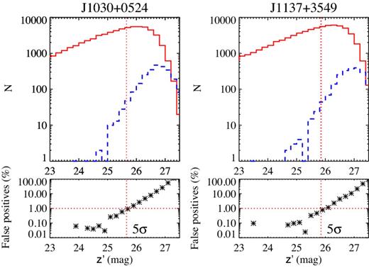
Top: distribution of z′-band magnitudes of sources in the field J1030+0524 (left) and J1137+3549 (right). The red solid line corresponds to the positive image and the blue dashed line corresponds to the negative image. The vertical dotted line shows the 5σ limit from Table 2. Bottom: percentage of false detection per magnitude bin obtained as the ratio of detections in the negative image over detections in the positive image. The horizontal dotted line indicates the 1 per cent contamination level. In both cases, a magnitude-limited sample (|$m_{z^{\prime }} \le m_{5\sigma }$|) has less than 1 per cent of contamination from false-positive detections.
APPENDIX B: SIMULATED OBSERVATIONS OF LBGs
Section 3.1 shows that, for this study, the influence of the UV spectral slope on the colours of galaxies is negligible. We also show that the Lyα forest attenuation and Lyα emission can significantly affect the colours of galaxies in the redshift range z = 5.5–5.9, using the filters in this work. Therefore, we adopt a value β = −2.0 for the LBG templates (see Section 3.1.1 for a description of the templates) and we simulate the observations of objects with Lyα equivalent widths from −10 to 200 Å using 10 Å steps. Each spectrum was redshifted from z = 4 to 6.5 using a step Δz = 0.01. At each step, the spectra were scaled to simulate MUV = −24.0 to −19.5 mag using a step ΔMUV = 0.1 mag. Then, magnitudes in the three filters Rc, i′ and z′ were computed using the throughput function of each filter, including filter transmission, atmospheric transmission at airmass = 1.2, quantum efficiency of the detector, transmission of the primary focus unit and primary focus reflectivity.
The typical size of bright LBGs at z > 5, defined by the average half-light radius, is rhl ∼ 0.15 arcsec (≲1 kpc; Bouwens et al. 2004; Oesch et al. 2010; Malhotra et al. 2012; Huang et al. 2013). However, the FWHM of the PSF in the PSF-equalized science images is 0.87 arcsec (1.13 arcsec) in the field J1030+0524 (J1137+3549), and not enough to spatially resolve most of these objects. Therefore, we use point sources to simulate the observations. For each realization described above, 100 point sources were added randomly distributed across the images, but avoiding superposition with real sources. The resulting number of simulated sources was 11 700 at each step of Lyα equivalent width. After applying the same extraction process and calibration as to the real objects, observed magnitudes were obtained and used to define an optimal selection of targets based on broad-band colours (see Section 3.2).
B1 Recovered objects and detection completeness
This section explores the limits imposed by the quality of the data. First, we present the precision of the magnitudes recovered from the simulations. Secondly, we show the range in redshift and MUV that is sampled with the observational data.
We compare the distribution of the residual magnitude measured in a 2 arcsec aperture minput − mrecovered, in each of the three photometric bands in the field J1030+0524, for objects in the redshift range z = 5.2–6.2 (i.e. 〈z〉 = 5.7, Δz = 1). Considering the model with Lyα in absorption, 90 per cent of the objects with S/N ≥ 5 are recovered with a precision of ±0.22 mag in the Rc band, ±0.14 mag in the i′ band and ±0.06 mag in the z′ band. Since the input magnitudes were calculated after calibrating the z′-band magnitude, the spread in i′ and Rc is dominated by the higher end of the redshift range considered (5.2 < z < 6.2), where Lyα has been redshifted to the z′ band and the Lyα forest and Lyman break have been redshifted to the i′ band and Rc band, respectively. In contrast, the spread in z′ is imposed by the quality of the data.
Fig. B1 presents the fraction of recovered objects per MUV bin and per z′-band magnitude bin as measured in an automatic aperture (MAG_AUTO) from the best seeing images. Black and grey lines correspond to 5σ and 3σ detections, respectively, of the model with Lyα in absorption. Three redshift ranges are plotted for comparison. In Fig. B1, more than 90 per cent of the galaxies with MUV ≤ −21.35 mag (−21.05 mag) are detected in the J1030+0524 (J1137+3549) field with S/N ≥ 5, at the three redshift bins. If objects with S/N ≥ 3 are included, the 90 per cent recovery limit moves to MUV = −20.9 mag (−20.60 mag), i.e. half a magnitude fainter. The three redshift ranges have different depths because the limit is imposed by the apparent magnitude in the z′ band, which correspond to brighter MUV for higher redshift. This effect is shown in the right-hand panels of Fig. B1 where the three redshift ranges show the same distribution of the recovery fraction as a function of z′ magnitude. In this plot, the vertical red dotted line indicates the m5σ limiting magnitude estimated in Section 2.3 (Table 2). The figure shows that |$z^{\prime }_{5\sigma }$| represents the magnitude at which the fraction of objects with S/N ≥ 5 drops to 50 per cent. If detections with S/N ≥ 3 are included, the fraction of recovered objects remains ≥90 per cent for magnitudes z′ ≥ |$z^{\prime }_{5\sigma }$|. However, in Section 3.2 only objects with S/N ≥ 5 are used to define the colour selection.
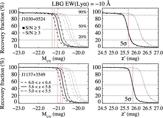
Fraction of recovered artificial LBGs as a function of absolute UV magnitude (λrest ∼ 1350 Å) (left) and apparent magnitude z′ (right). The black lines correspond to a sample detected with S/N ≥ 5 and the grey lines correspond to S/N ≥ 3. The dashed, solid and dot–dashed lines show the distribution of objects at different redshift bins. In the left-hand panels, the horizontal dotted lines indicate the 90, 50 and 20 per cent levels of completeness, and the vertical dotted lines correspond to the UV magnitudes with 90 per cent level of completeness. For the J1030+0524 field (top), the 90 per cent completeness of each redshift sample is MUV = −21.32 (dashed), −21.20 (solid) and −21.05 (dot–dashed), and for the J1137+3549 field (bottom) the corresponding values are MUV = −21.05 (dashed), −20.9 (solid) and −20.8 (dot–dashed). In the right-hand panels, the vertical dotted line shows the 5σ-limiting magnitude from Table 2. The recovery fraction of the sample with S/N ≥ 5 is 50 per cent at a magnitude |$z^{\prime }_{5\sigma }$|, which means that a 5σ-limited sample recovers 50 per cent of the objects with magnitudes z′ = |$z^{\prime }_{5\sigma }$|.
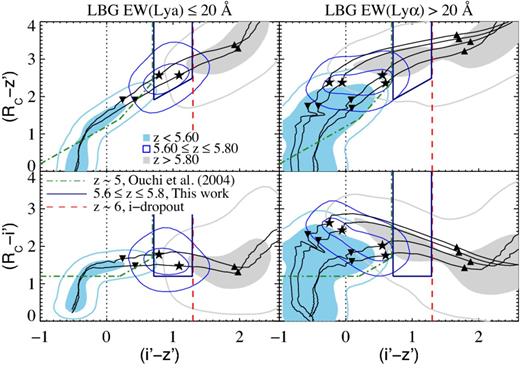
Colour–colour diagrams of recovered LBGs. Left-hand panels show LBGs with EW(Lyα) ≤ 20 Å and right-hand panels show LBGs with EW(Lyα) > 20 Å. The contours show the distribution of the colours according to the redshift of the input source. Light blue filled contours show z < 5.68, grey filled contours show z > 5.78 and blue line contours show the range 5.68 ≤ z ≤ 5.78. Colour–colour space selection criteria are delimited: z ∼ 6 i′-dropouts (red dashed lines), z ∼ 5 Ri′z′-LBGs (green dot–dashed lines) and z ∼ 5.7 LBGs of this work (blue solid lines). The black tracks correspond to the LBG templates used to generate input fake sources. The tracks in left-hand panels have EW(Lyα) = −10 and 20 Å, and the tracks in the right-hand panels have EW(Lyα) = 30, 50, 150 and 200 Å. The plots show that among galaxies with EW(Lyα) ≤ 20 Å (left-hand panels) those in the narrow redshift range of interest (blue line contours) are expected to dominate the colour window adopted for this work (blue solid lines) whereas the number of galaxies at lower/higher redshift in this window is expected to be low. Moreover, for galaxies with EW(Lyα) > 20 Å (right-hand panel), the number of objects in the redshift range of interest (blue line contours) found in the colour window drops significantly. Thus, the colour window shown by the solid lines can select a sample of galaxies with EW(Lyα) ≤ 20 Å, thus complementary to z ∼ 5.7 LAEs which by definition have EW(Lyα) > 20 Å.
Interestingly, the right-hand panels show that the population of LBGs with EW(Lyα) > 20 Å at 5.68 ≤ z ≤ 5.78 is shifted from the mentioned colour window. In addition, the contamination from higher redshift objects remains low. Therefore, the window defined by equations (B1) and (B2) opens the opportunity to explore a selection criterion that targets LBGs with EW(Lyα) ≤ 20 Å (or non-LAEs) in the redshift of interest z ∼ 5.7. We will refer to this colour–colour window as z ∼ 5.7 LBG colour criteria.
Fig. B3 shows in better detail the gap in redshift space left by the i′-dropout (red dashed line) and the Ri′z′-LBG selection (green dot–dashed line) in the field J1030+0524. In the left-hand panel, the fraction of recovered LBGs with EW(Lyα) ≤ 20 Å using equations (B1) and (B2) (blue solid line) reaches 80 per cent at the redshift of the C iv systems (blue long-dashed vertical lines). Coincidentally, the minimum recovery fraction of the other selection criteria is reached at the redshift of the C iv systems. The recovery fraction is ≥50 per cent in the redshift range 5.627–5.830 (Δz ∼ 0.2), which corresponds to a comoving line-of-sight length of ∼90 h−1 comoving Mpc. Hence, the z ∼ 5.7 LBG colour criteria select LBGs in a narrow redshift range centred in the redshift of the C iv absorption systems of interest. Now that the colour–colour region of interest has been identified, it is important in understanding the nature of the contaminant sources in the colour selection window to explore additional constraints in the selection to produce a cleaner sample. The next section presents the contamination sources and their expected impact on the selection of LBGs, as well as the additional conditions used to select high-redshift galaxies.
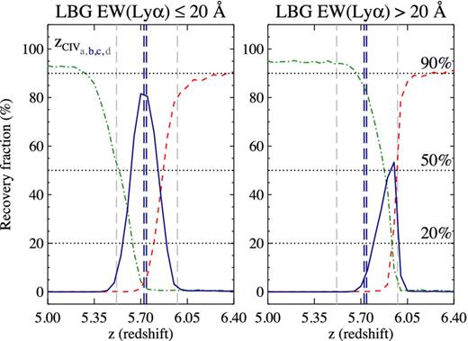
Fraction of recovered artificial LBGs as a function of redshift. This figure shows that the selection criteria adopted for this work cover the window in redshift that is left by the selection criteria of LBGs at z ∼ 5 and z ∼ 6. Moreover, this redshift window corresponds to the redshift of the two z ∼ 5.7 C iv absorption systems in the field. In order to consistently compare the evolution with redshift, only objects with MUV ≤ −21.5 are included. Green dot–dashed, red dashed and dark blue solid curves correspond to objects selected with the z ∼ 5 Ri′z′-LBG selection of Ouchi et al. (2004a), the z ∼ 6 i-dropout criteria and the z ∼ 5.7 LBG selection from this work, respectively. The left-hand panel shows that the fraction of LBGs with EW(Lyα) ≤ 20 Å selected with the colour window described in Section 3.2 is maximum at the redshift of the C iv systems. The right-hand panel shows that LBGs with EW(Lyα) > 20 Å selected with the colour criteria for this work lie at higher redshift (z ∼ 5.9). This source of contaminants, however, is low and can be easy to identify from spectroscopy due to the Lyα emission line.
APPENDIX C: CONTAMINATION IN THE z ∼ 5.7 LBG SAMPLE
The contamination in the colour selection for z ∼ 5.7 LBGs (equations B1 and B2) comes from two main sources: Galactic M stars and elliptical galaxies in the redshift range z = 1.2–1.8. In this section, we analyse the contamination expected from each of these sources and we present additional conditions to select z ∼ 5.7 LBGs. We close the section with the contamination from background fluctuations.
C1 Galactic stars
Given the colours and small sizes of z ∼ 5–6 LBGs, stars can be an abundant source of contamination. Fortunately, they occupy a well-defined region in typical colour–colour diagrams used to select z ∼ 6 galaxies (Fig. C1). Because we are selecting sources with colours that are typical of late-type stars, the contamination from Galactic low-mass stars can be high. Fig. C1 presents the colours of cool low-mass stars from West et al. (2008) obtained from the SDSS. They occupy a narrow stripe that runs through the colour window of z ∼ 5.7 LBGs (blue solid line). The black solid lines are the same LBG tracks as in the left-hand panels of Fig. B2 and the filled stars indicate z = 5.7. The Sloan r′ band is plotted instead of the Rc band used in this work. However, the number of contaminants estimated below is for the z′-band magnitude. In particular, the right-hand panel of Fig. C1 presents (i′ − z′) versus spectral type and shows that the stars inside the selection window (red filled contours) have spectral types in the range M2–M8. The figure also shows the position of L and T dwarfs from Metchev et al. (2008, inverted triangles). All stars colder than M8 have redder (i′ − z′) colours and, therefore, are not sources of contamination for the z ∼ 5.7 LBGs.
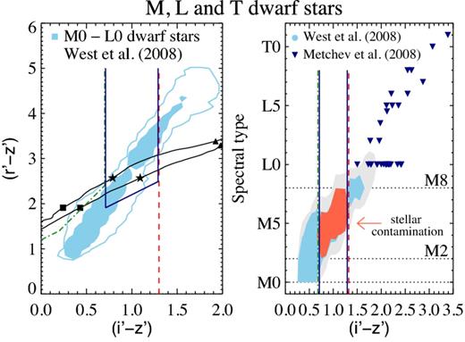
Left: Colour–colour diagrams (r′ − z′) – (i′ − z′) and (r′ − i′) – (i′ − z′) for M stars from West et al. (2008, contours). Green dot–dashed, red dashed and dark blue solid lines denote the colour criteria described in Fig. B2. This figure shows that stars cross through the window in colour–colour space occupied by the targeted LBG population (filled stars in black solid tracks, same as Fig. B2). Right: spectral type as a function of (i′ − z′). Light blue filled contours show M0–L0 stars from West et al. (2008) and dark blue triangles denote L and T dwarfs from Metchev et al. (2008). All stars in the z ∼ 5.7 LBG colour selection window are indicated with red filled contours. The stellar contamination comes from stars in the spectral type range M2–M8.
In order to estimate the number of cool stars expected to contaminate our sample, we identify the absolute magnitude range and distance range of the contaminant stars. First, the absolute magnitude in the z′ band of the M stars with colours 0.7 ≤ (i′ − z′) ≤ 1.3 was obtained from the colour–absolute magnitude relation of Bochanski et al. (2010, table 4 of their paper, but see the Erratum Bochanski et al. 2012). Secondly, from the absolute magnitudes of the contaminant stars, we estimate the range of distances d = 2.38–22.64 kpc to meet the apparent magnitude range of interest, for our z ∼ 5.7 galaxies. The galactic coordinates of fields J1030+0524 and J1137+3549 are l = 239.4549 b = 50.0511 and l = 179.4436 b = 71.9995, respectively. Thus, both fields are above the 45° of galactic latitude (well above the Galactic plane) and would include mainly the inner halo of the Milky Way and the high end of the thick disc (Brown et al. 2004; Carollo et al. 2007).
A rough estimate of the number density of stars was obtained from a simple model of the Galaxy. We adopted a thin disc + thick disc model from Bochanski et al. (2010), for distances smaller than 2000 pc above the plane of the galaxy. Then, for heights Z > 2000 pc, the model adopted was the best-fitting thin disc + thick disc model of Jurić et al. (2008) for faint and red stars (1.3 < (r′ − i′) < 1.4; table 4 of Jurić et al. 2008) with the additional halo distribution they obtained for a slightly bluer sample (0.9 < (r′ − i′) < 1.0). Finally, the density of stars in each distance bin is obtained from the models. The volume contained in the field of view at each distance bin is used to estimate the total number of stars expected in each absolute magnitude bin. Then, the distance is used to convert it to apparent z′ magnitude bin.
Fig. C2 shows the average number of Galactic contaminant stars expected in each field (solid lines) per 0.5 apparent magnitude in the range of magnitudes of interest. To generate the histogram, we corrected the expected number of stars described above for the sensitivity in the z′ band by multiplying by the recovery fraction of objects as a function of z′ (Fig. B1). Hence, we obtain the equivalent of a magnitude-limited sample. Overplotted with dashed lines are the total number of objects detected with S/N ≥ 5 (error-limited sample) and selected with the z ∼ 5.7 LBG criteria. The dotted vertical lines indicate the 5σ detection limits of each field. The comparison with this toy model shows that the number of detections is larger than the expected average stellar contaminations, meaning that other types of sources also inhabit the colour region. The exceptions are the faintest bins, which show the effect of the comparison between a magnitude-limited sample expected from a toy model and an error-limited observed sample like the z ∼ 5.7 LBGs of this work. In a magnitude-limited sample, the 5σ-limiting magnitude is the magnitude at which 50 per cent of the objects are recovered whereas in an error-limited sample, the 5σ-limiting magnitude is the faintest average magnitude with S/N = 5, i.e. the magnitude of the faintest object.
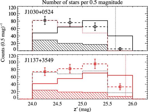
Number of stars per apparent magnitude bin estimated in each field using models for the distribution of stars from Bochanski et al. (2010) and Jurić et al. (2008). The solid line histogram corresponds to the predicted number of stars corrected for the sensitivity of our data. The dashed line histogram shows the total number of observed sources in the colour selection window for z ∼ 5.7 LBGs. The error bars correspond to Poisson and photometric errors. The line-filled histogram corresponds to observed objects with S/G|$_z^{\prime }>0.9$| and shows a significant difference from the predicted number of stars. Finally, the dotted line histogram corresponds to all the sources rejected by our z ∼ 5.7 LBG selection criteria (Section 3.2).
Comparing the dashed line histogram in each panel of Fig. C2, the number of objects selected in the field J1030+0524 drops towards the 5σ detection limit whereas the opposite is observed in the field J1137+3549. The reason is that the i′-band image of the field J1030+0524 is 0.42 mag deeper than the i′-band image of the J1137+3549 field. However, the detection image of the field J1030+0524 is 0.2 mag shallower than that of J1137+3549 (Table 2). As a result, the excess of sources in the field J1137+3549 is dominated by photometric errors. Many 5σ detections in this field have colours with lower signal-to-noise.
One approach to effectively minimize the number of Galactic stars is to simply avoid the well-defined stellar locus in our colour–colour plots but this would also remove a significantly large number of z ∼ 5.7 galaxies. Therefore, to minimize the contamination from stars, we opted for the standard approach and included a condition in the star-to-galaxy (S/G) classification from SExtractor in the detection image: S/G|$_{z^{\prime }}<0.9$|. This condition aims to remove objects with the highest probability of being a star. However, the filled histograms in Fig. C2 correspond to objects with S/G|$_{z^{\prime }}\ge 0.9$| and, in both fields, they are significantly lower than the predicted number of stars (solid line histogram). This indicates that many stars have S/G|$_{z^{\prime }}<0.9$| and therefore additional conditions are needed to remove further stars. We added a restriction on the isophotal area in the Rc band (ISO_AREA_Rc < 22 pixel2) which also reduces the contamination from low-redshift red galaxies. We discuss galaxy contamination in the following subsection.
C2 Red and evolved galaxies
The 4000 Å Balmer break present in the spectrum of evolved galaxies at redshift z = 1.05 would be observed at λ ∼ 8200 Å and could mimic the Lyα break due to Lyα forest in the spectrum of a z ∼ 5.7 LBG. Fig. C3 presents in the top panel the evolution with redshift of the (Rc − z′) and (i′ − z′) colours of five different templates of red and evolved galaxies. The long-dashed and dotted tracks correspond to the synthetic model template spectrum of a typical ES0 galaxy and a more evolved elliptical galaxy, respectively, from the Bruzual & Charlot (2003) synthesis model. Open stars indicate redshift values z = 0.9, 1.1, 1.3, 1.5, 1.7 and 1.9, for comparison with the composite spectra of observed galaxies. The red, green and blue solid tracks correspond to the early-, intermediate- and late-type galaxy composite spectra of the Gemini Deep Deep Survey (GDDS; Abraham et al. 2004). All tracks were calculated using the transmission curve of Suprime-Cam filters. The red track samples the redshift range z = 0.92-1.70, the green track samples z = 0.96-1.48 and the blue track samples z = 1.12-2.15. A comparison of the tracks shows that GDDS early and intermediate templates are fairly approximated by the ES0 synthetic template (long-dashed track) at the corresponding redshift (0.9 ≤ z ≤ 1.5, open stars), while a more evolved stellar population (dotted track) will not reach the colour tracks of observed early-type galaxies. Finally, the late-type galaxy template is very distant from the window of interest in the colour–colour diagram. Thus, the more likely source of extragalactic contaminants in the colour–colour window of interest is galaxies of early to intermediate type.
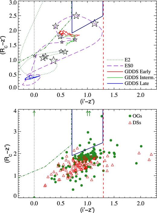
(Rc − z′)–(i′ − z′) colour–colour diagram of red galaxies. The green dot–dashed, red dashed and dark blue solid lines show the colour criteria described in Fig. B2. Top: redshift evolution of the colours of the early-type (red solid track), intermediate-type (green solid track) and late-type (blue solid track) galaxy composite spectra of GDDS. The colours of synthetic model spectra of a typical ES0 (purple dashed track) and an old elliptical (green dotted track) are shown for comparison. The redshift range probed by the GDDS templates is highlighted with stars. Open stars from small to large indicate redshifts z = 0.9, 1.1, 1.3, 1.5, 1.7 and 1.9. The ES0 track approaches the red and green tracks at the redshift of the galaxies used in the composites (z ∼ 0.9–1.5). Only early- and intermediate-type galaxies inhabit the proximity of the colour selection for z ∼ 5.7 LBGs. Bottom: colour–colour diagram of the ERO sample. Green solid circles show objects classified as old galaxies and red open triangles correspond to dusty starbursts (Miyazaki et al. 2003). The contamination in the colour window is dominated by old galaxies, in agreement with the top plot.
The bottom panel of Fig. C3 presents the colour–colour diagram of 247 extremely red objects (EROs) of Miyazaki et al. (2003). EROs classified as ‘old galaxies’ (OGs) are green filled circles and ‘dusty starbursts’ (DSs) are red open triangles. Only 11 EROs are found inside the colour window for z ∼ 5.7 LBGs and they represent 4.4 per cent of the total sample of Miyazaki et al. (2003). Specifically, nine of them are classified as OGs and two of them as DSs, suggesting that the contamination is dominated by evolved galaxies rather than ‘starburst-type’ galaxies, in agreement with the result from GDDS data.
Fig. C4 shows the (Rc − z′) versus z′ colour–magnitude diagram and the apparent z′ magnitude distribution of EROs (bottom panel). Open black circles represent the total population and red triangles show the sources that contaminate the colour window, which are among the reddest objects in the sample. The limiting magnitude of the EROs sample is |$z^{\prime }_{\rm lim} = 25$| mag (Miyazaki et al. 2003), and if we compare the magnitude distribution of EROs with the bright end of the luminosity function of LBGs at z ∼ 6 (z′ ∼ 24 mag), we find that only 1.6 per cent EROs are red enough to contaminate the colour selection. This is shown in the bottom panel of Fig. C4 that presents the magnitude distribution of the EROs sample (black solid histogram) and the sub-sample that contaminates the colour–colour window (red filled histogram). Four objects are as faint as the expected high-redshift LBGs; all of them are classified as OGs.
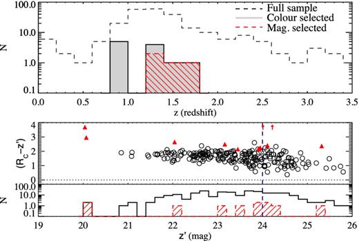
Top: redshift distribution of the ERO sample. The black dashed histogram corresponds to the total sample of EROs from Miyazaki et al. (2003), the grey filled histogram indicates the redshift of EROs in the colour–colour window of z ∼ 5.7 LBGs and the red filled histogram shows the sub-sample fainter than z′ = 24.0. The more likely source of contaminants seems to be in the redshift range 1.2 < z < 1.8. Bottom: (Rc − z′) – z′ colour–magnitude diagrams and z′-band magnitude distribution of EROs. Contaminants of the colour selection window are plotted with red solid triangles in the colour–magnitude diagram and red filled histogram in the magnitude distribution plot. All contaminants are the reddest objects of the sample and only 4 of the 11 contaminant objects from the ERO sample are as faint as z > 5 LBGs.
The photometric redshifts of the EROs sample are plotted in the top panel of Fig. C4. The dashed lines correspond to the total sample and the solid line-filled histograms correspond to objects in the colour–colour window of z ∼ 5.7 LBGs. The red dashed filled histogram shows the redshift of the four objects that also meet the z′-band magnitude criterion of z ∼ 5.7 LBGs and suggests that the more likely source of contaminants is in the redshift range 1.2 < z < 1.8. This range corresponds approximately to the redshift indicated by the four largest stars of the long-dashed track in the top panel of Fig. C3.
In summary, the contamination from red galaxies seems to be dominated by relatively old galaxies with spectroscopic features of early to intermediate type. Contamination maximizes in the redshift range 1.2 < z < 1.8 in which the observation with broad-band photometry of the 4000 Å Balmer break can simulate the effect of the Lyα forest in LBGs at z > 5. Furthermore, only galaxies fainter than z′ ≥ 24.0 mag are possible contaminants and the expected population of this type of galaxies at 1.2 < z < 1.8 is not well known. Therefore, we can only attempt to remove this source of contamination using a size-limited sample.
Considering the distribution of effective radius Re of LBGs at z > 5, which has been found smaller than 1.5 kpc (or 0.45 arcsec), with a mean 〈Re〉 ∼ 0.15 arcsec (e.g. Bouwens et al. 2006; Huang et al. 2013), we include a condition in the half-light radius measured with SExtractorrhl ≤ 4.5 arcsec. Additional conditions to remove lower redshift old galaxies are photometric area in the Rc band < 22 pixel2 and S/G|$_{z^{\prime }}\ge$| 0.01. Spectroscopy follow-up of sources detected has been obtained and data are being reduced. Thus, a more accurate estimate of the contamination level of the selection criteria will be presented in a forthcoming paper.
C3 False detections from background fluctuations
The histogram in Fig. C5 shows the distribution of photometric errors in the science images (solid) and the negative images (dashed). The contamination of false detections defined as the fraction of false positives per error bin (bottom panel) reaches ∼1 per cent for a detection magnitude error of ∼0.27 mag in both fields. For sources with S/N ≥ 5 (5σ), the fraction is less than 0.1 per cent. In other words, in a 5σ-limited sample less than 1 detection in every 1000 sources is a noise fluctuation of the background. Therefore, we limit our sample to sources with S/N ≥ 5 and neglect this source of error.
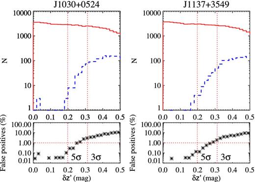
Top: distribution of photometric errors in the fields J1030+0524 (left) and J1137+3549 (right). The red solid histogram corresponds to the positive image and the blue dashed histogram corresponds to the negative image. Bottom: percentage of false detection per error bin obtained as the ratio of detections in the negative image over detections in the positive image. The horizontal dotted line indicates the 1 per cent contamination level. The vertical dotted line indicates the error of a 5σ and 3σ detection, i.e. 0.198 and 0.312 mag, respectively. In both cases, a sample limited by S/N ≥ 5 (|$\delta m_{z^{\prime }} \le 0.198$|) has less than 0.1 per cent of contamination from false-positive detections.
APPENDIX D: SELECTION PROBABILITY FUNCTION
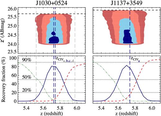
Top: selection probability function P(m, z) of the z ∼ 5.7 LBG selection introduced in this study. The contours (outside-in) indicate probabilities of selection (including detection) of 0.1, 0.25, 0.5 and 0.75. Bottom: fraction of recovered objects as a function of redshift obtained from the simulated observation of 10 000 LBGs in each field and at each redshift step (Δz = 0.01). The green dot–dashed line corresponds to objects recovered with the colour selection for Rci′z′-LBGs of Ouchi et al. (2004a). The red dashed line corresponds to i′-dropout colour selected objects and the blue solid line corresponds to objects recovered with the z ∼ 5.7 LBG criteria. In both fields, the blue line peaks at z ∼ 5.7 and the width at half-maximum is ∼0.2. The vertical long-dashed lines show the redshift of the C iv systems known to date at z > 5 in each field. In the left-hand panel, the blue long-dashed lines indicate the redshift of two C iv systems at zabs = 5.7242 and 5.7428 (Ryan-Weber et al. 2009; Simcoe 2011). The grey long-dashed lines indicate the systems at zabs = 5.5172 (Simcoe 2011; D'Odorico et al. 2013) and zabs = 5.9757 (D'Odorico et al. 2013). In the right-hand panel, the blue long-dashed vertical line indicates the redshift of one C iv system at zabs = 5.7383 (Ryan-Weber et al. 2009). This work focuses on objects in the environment of the zabs ∼ 5.7 C iv systems only.
APPENDIX E: MAGNITUDES AND COLOURS OF LBGs
z ∼ 5.7 LBGs – J1030+0524.
| RA (J2000) | Dec. (J2000) | Rc (2 arcsec) | i′ (2 arcsec) | z′ (2 arcsec) | NB|$_{{C\,{\small {IV}}}}$| (2 arcsec) | z′ (MAG_AUTO) | rhl (pixels) | S/G|$_{z^{\prime }}$| |
|---|---|---|---|---|---|---|---|---|
| 10:29:34.05 | +05:36:09.6 | ≳28.35 | 26.32 ± 0.32 | 25.25 ± 0.32 | 25.96 ± 0.45 | 25.38 ± 0.16 | 1.99 | 0.82 |
| 10:29:36.17 | +05:25:44.1 | 27.37 ± 0.50 | 26.05 ± 0.26 | 25.03 ± 0.27 | 25.94 ± 0.45 | 25.10 ± 0.14 | 2.06 | 0.2 |
| 10:29:39.44 | +05:27:38.8 | 27.26 ± 0.46 | 26.04 ± 0.26 | 24.89 ± 0.24 | 25.48 ± 0.31 | 24.97 ± 0.11 | 2.08 | 0.81 |
| 10:29:44.06 | +05:14:27.8 | 27.56 ± 0.58 | 26.35 ± 0.33 | 25.40 ± 0.36 | 25.84 ± 0.41 | 25.47 ± 0.19 | 2.15 | 0.26 |
| 10:29:47.74 | +05:37:16.6 | 27.74 ± 0.66 | 26.26 ± 0.31 | 25.25 ± 0.32 | 26.12 ± 0.51 | 25.29 ± 0.16 | 2.12 | 0.47 |
| 10:29:51.01 | +05:09:07.8 | ≳28.35 | 26.46 ± 0.36 | 25.38 ± 0.36 | 26.15 ± 0.52 | 25.49 ± 0.19 | 1.94 | 0.6 |
| 10:29:51.67 | +05:26:50.0 | 27.53 ± 0.56 | 26.24 ± 0.30 | 25.45 ± 0.38 | 25.84 ± 0.41 | 25.51 ± 0.19 | 1.99 | 0.89 |
| 10:29:53.43 | +05:27:18.3 | ≳28.35 | 26.63 ± 0.41 | 25.52 ± 0.40 | 26.50 ± 0.67 | 25.57 ± 0.19 | 2.05 | 0.62 |
| 10:29:56.18 | +05:18:48.9 | 27.36 ± 0.50 | 25.67 ± 0.19 | 24.62 ± 0.19 | 25.20 ± 0.25 | 24.64 ± 0.09 | 2.12 | 0.81 |
| 10:29:59.19 | +05:34:46.4 | 27.76 ± 0.66 | 26.26 ± 0.31 | 25.38 ± 0.36 | 26.04 ± 0.48 | 25.38 ± 0.17 | 2.11 | 0.88 |
| 10:30:06.72 | +05:16:48.8 | 27.26 ± 0.46 | 25.58 ± 0.18 | 24.78 ± 0.22 | 25.39 ± 0.29 | 24.84 ± 0.11 | 2.14 | 0.41 |
| 10:30:06.88 | +05:19:22.3 | 27.13 ± 0.42 | 25.68 ± 0.19 | 24.82 ± 0.23 | 24.91 ± 0.20 | 24.94 ± 0.12 | 1.95 | 0.34 |
| 10:30:06.91 | +05:39:05.6 | ≳28.35 | 26.33 ± 0.32 | 25.36 ± 0.35 | 25.69 ± 0.37 | 25.49 ± 0.18 | 2.05 | 0.76 |
| 10:30:07.75 | +05:20:44.0 | 27.77 ± 0.67 | 26.32 ± 0.32 | 25.37 ± 0.35 | ≳27.49 | 25.49 ± 0.18 | 1.96 | 0.61 |
| 10:30:12.71 | +05:19:07.8 | 27.57 ± 0.58 | 26.14 ± 0.28 | 25.15 ± 0.30 | 26.24 ± 0.56 | 25.15 ± 0.15 | 2.22 | 0.39 |
| 10:30:13.79 | +05:15:00.6 | ≳28.35 | 26.48 ± 0.37 | 25.47 ± 0.38 | ≳27.49 | 25.53 ± 0.19 | 2.07 | 0.89 |
| 10:30:16.30 | +05:32:36.6 | 27.85 ± 0.70 | 26.10 ± 0.27 | 25.02 ± 0.27 | 25.88 ± 0.43 | 25.08 ± 0.13 | 2.09 | 0.59 |
| 10:30:18.93 | +05:18:33.9 | 27.73 ± 0.65 | 26.21 ± 0.29 | 25.46 ± 0.38 | 25.92 ± 0.44 | 25.53 ± 0.19 | 2.07 | 0.33 |
| 10:30:19.80 | +05:17:53.0 | 27.44 ± 0.53 | 26.03 ± 0.25 | 24.79 ± 0.22 | 25.51 ± 0.32 | 24.86 ± 0.11 | 2.03 | 0.24 |
| 10:30:21.45 | +05:36:49.9 | ≳28.35 | 25.94 ± 0.24 | 24.92 ± 0.25 | 24.53 ± 0.14 | 24.93 ± 0.13 | 2.21 | 0.55 |
| 10:30:35.45 | +05:24:20.5 | 27.60 ± 0.59 | 26.10 ± 0.27 | 25.29 ± 0.33 | 26.45 ± 0.65 | 25.34 ± 0.15 | 1.96 | 0.81 |
| 10:30:41.26 | +05:17:53.6 | 27.86 ± 0.71 | 26.17 ± 0.29 | 25.21 ± 0.31 | 26.12 ± 0.51 | 25.25 ± 0.16 | 2.1 | 0.67 |
| 10:30:46.12 | +05:11:23.0 | ≳28.35 | 26.10 ± 0.27 | 24.93 ± 0.25 | 25.35 ± 0.28 | 24.99 ± 0.16 | 2.18 | 0.86 |
| 10:30:47.84 | +05:11:58.3 | 27.89 ± 0.72 | 25.87 ± 0.22 | 24.57 ± 0.18 | 25.13 ± 0.24 | 24.61 ± 0.09 | 2.16 | 0.44 |
| 10:30:48.69 | +05:26:37.3 | 27.39 ± 0.51 | 25.87 ± 0.22 | 24.88 ± 0.24 | 25.80 ± 0.40 | 24.94 ± 0.12 | 2.15 | 0.62 |
| 10:30:50.36 | +05:35:06.0 | 27.40 ± 0.51 | 25.90 ± 0.23 | 24.85 ± 0.23 | 25.83 ± 0.41 | 24.95 ± 0.14 | 2.22 | 0.09 |
| 10:30:52.61 | +05:08:05.9 | ≳28.35 | 26.38 ± 0.34 | 25.39 ± 0.36 | 26.06 ± 0.49 | 25.38 ± 0.17 | 2.23 | 0.38 |
| 10:30:53.95 | +05:32:32.9 | ≳28.35 | 26.02 ± 0.25 | 25.18 ± 0.30 | 26.00 ± 0.47 | 25.24 ± 0.16 | 2.18 | 0.4 |
| 10:31:02.36 | +05:33:08.1 | 27.72 ± 0.65 | 26.08 ± 0.26 | 25.25 ± 0.32 | 25.55 ± 0.33 | 25.31 ± 0.17 | 2.11 | 0.27 |
| 10:31:02.97 | +05:14:21.0 | ≳28.35 | 25.95 ± 0.24 | 25.14 ± 0.29 | 26.27 ± 0.57 | 25.24 ± 0.16 | 2.11 | 0.55 |
| 10:31:10.51 | +05:25:52.9 | 27.18 ± 0.44 | 25.94 ± 0.24 | 24.78 ± 0.22 | 25.57 ± 0.34 | 24.83 ± 0.11 | 2.2 | 0.17 |
| 10:31:11.22 | +05:14:43.7 | 26.99 ± 0.38 | 25.43 ± 0.15 | 24.70 ± 0.20 | 25.18 ± 0.24 | 24.76 ± 0.11 | 2.16 | 0.53 |
| 10:31:17.39 | +05:17:32.2 | 27.61 ± 0.60 | 26.05 ± 0.26 | 24.99 ± 0.26 | 26.24 ± 0.56 | 25.07 ± 0.13 | 2.05 | 0.88 |
z ∼ 5.7 LBGs – J1137+3549.
| RA (J2000) | Dec. (J2000) | Rc (2.4 arcsec) | i′ (2.4 arcsec) | z′ (2.4 arcsec) | NB|$_{{C\,{\small {IV}}}}$| (2.4 arcsec) | z′ (MAG_AUTO) | rhl (pixels) | S/G|$_{z^{\prime }}$| |
|---|---|---|---|---|---|---|---|---|
| 11:36:04.48 | +35:42:50.3 | ≳28.00 | 26.54 ± 0.45 | 25.62 ± 0.45 | ≳27.39 | 25.65 ± 0.18 | 1.92 | 0.37 |
| 11:36:05.05 | +35:42:51.1 | 27.20 ± 0.53 | 25.96 ± 0.29 | 25.24 ± 0.34 | 25.75 ± 0.44 | 25.26 ± 0.15 | 2.2 | 0.18 |
| 11:36:09.38 | +35:52:08.7 | ≳28.00 | 25.68 ± 0.23 | 24.75 ± 0.23 | 25.16 ± 0.28 | 24.69 ± 0.08 | 2.14 | 0.44 |
| 11:36:10.19 | +35:55:25.0 | 26.83 ± 0.41 | 25.60 ± 0.21 | 24.78 ± 0.23 | 24.97 ± 0.24 | 24.82 ± 0.09 | 2.12 | 0.88 |
| 11:36:10.22 | +35:45:29.8 | 27.48 ± 0.65 | 26.11 ± 0.33 | 24.90 ± 0.25 | 25.86 ± 0.47 | 24.95 ± 0.1 | 2.05 | 0.81 |
| 11:36:10.91 | +35:46:48.1 | ≳28.00 | 26.35 ± 0.39 | 25.42 ± 0.39 | ≳27.39 | 25.38 ± 0.17 | 2.2 | 0.04 |
| 11:36:14.96 | +35:45:05.0 | 27.08 ± 0.49 | 25.55 ± 0.21 | 24.45 ± 0.18 | 25.15 ± 0.27 | 24.45 ± 0.07 | 2.23 | 0.18 |
| 11:36:15.05 | +35:44:56.0 | 27.53 ± 0.67 | 26.19 ± 0.35 | 25.27 ± 0.34 | ≳27.39 | 25.35 ± 0.13 | 1.9 | 0.64 |
| 11:36:15.71 | +35:43:46.1 | ≳28.00 | 26.28 ± 0.37 | 25.21 ± 0.33 | 25.87 ± 0.48 | 25.43 ± 0.16 | 1.88 | 0.79 |
| 11:36:16.16 | +35:37:44.0 | 27.45 ± 0.64 | 25.88 ± 0.27 | 24.66 ± 0.21 | 25.28 ± 0.30 | 24.65 ± 0.08 | 2.19 | 0.18 |
| 11:36:22.50 | +35:45:04.7 | ≳28.00 | 26.79 ± 0.55 | 25.53 ± 0.42 | ≳27.39 | 25.56 ± 0.16 | 2.05 | 0.66 |
| 11:36:23.01 | +35:57:54.3 | 26.97 ± 0.45 | 25.49 ± 0.20 | 24.69 ± 0.22 | 25.37 ± 0.33 | 24.70 ± 0.09 | 2.16 | 0.24 |
| 11:36:23.04 | +35:56:35.0 | ≳28.00 | 26.34 ± 0.39 | 25.43 ± 0.39 | 25.80 ± 0.46 | 25.56 ± 0.17 | 2.07 | 0.29 |
| 11:36:23.77 | +35:38:28.1 | 27.14 ± 0.51 | 25.46 ± 0.19 | 24.47 ± 0.18 | 25.66 ± 0.41 | 24.46 ± 0.06 | 2.11 | 0.41 |
| 11:36:27.82 | +35:58:16.8 | ≳28.00 | 26.71 ± 0.51 | 25.50 ± 0.41 | 26.40 ± 0.70 | 25.58 ± 0.17 | 1.89 | 0.45 |
| 11:36:33.27 | +35:40:39.9 | ≳28.00 | 26.05 ± 0.31 | 25.20 ± 0.33 | 25.58 ± 0.39 | 25.23 ± 0.12 | 2.0 | 0.19 |
| 11:36:36.40 | +35:56:28.8 | ≳28.00 | 26.16 ± 0.34 | 24.92 ± 0.26 | 26.09 ± 0.56 | 24.91 ± 0.1 | 2.14 | 0.15 |
| 11:36:37.51 | +35:57:07.7 | ≳28.00 | 26.29 ± 0.38 | 25.09 ± 0.30 | 25.58 ± 0.38 | 25.15 ± 0.14 | 2.08 | 0.22 |
| 11:36:39.52 | +35:52:29.5 | 27.35 ± 0.59 | 26.05 ± 0.31 | 24.95 ± 0.27 | 26.02 ± 0.53 | 24.94 ± 0.1 | 2.04 | 0.54 |
| 11:36:41.69 | +35:44:40.3 | 27.56 ± 0.69 | 26.01 ± 0.30 | 24.79 ± 0.23 | 25.57 ± 0.38 | 24.73 ± 0.08 | 2.19 | 0.84 |
| 11:36:48.09 | +35:58:20.1 | ≳28.00 | 26.27 ± 0.37 | 25.31 ± 0.36 | 26.29 ± 0.65 | 25.38 ± 0.14 | 1.86 | 0.61 |
| 11:36:49.63 | +35:58:55.0 | ≳28.00 | 26.79 ± 0.54 | 25.77 ± 0.50 | ≳27.39 | 25.74 ± 0.2 | 2.19 | 0.3 |
| 11:36:53.00 | +35:39:14.8 | 27.05 ± 0.48 | 25.54 ± 0.20 | 24.54 ± 0.19 | 25.10 ± 0.26 | 24.51 ± 0.07 | 2.23 | 0.62 |
| 11:36:53.54 | +35:44:16.2 | 26.81 ± 0.40 | 25.60 ± 0.21 | 24.73 ± 0.22 | 25.54 ± 0.37 | 24.74 ± 0.08 | 2.03 | 0.86 |
| 11:36:54.53 | +36:02:12.8 | ≳28.00 | 26.41 ± 0.41 | 25.70 ± 0.48 | 25.89 ± 0.49 | 25.73 ± 0.19 | 2.01 | 0.62 |
| 11:36:56.06 | +35:57:43.6 | ≳28.00 | 25.95 ± 0.29 | 25.02 ± 0.28 | 25.95 ± 0.51 | 25.25 ± 0.13 | 2.01 | 0.85 |
| 11:36:57.16 | +35:57:46.3 | 27.44 ± 0.63 | 26.17 ± 0.34 | 25.41 ± 0.39 | ≳27.39 | 25.44 ± 0.14 | 1.84 | 0.75 |
| 11:36:58.77 | +35:46:06.3 | ≳28.00 | 26.69 ± 0.51 | 25.75 ± 0.50 | ≳27.39 | 25.74 ± 0.19 | 1.8 | 0.22 |
| 11:37:01.18 | +35:51:19.1 | ≳28.00 | 25.84 ± 0.26 | 25.02 ± 0.28 | 25.84 ± 0.47 | 25.05 ± 0.1 | 2.0 | 0.53 |
| 11:37:01.87 | +35:48:46.8 | ≳28.00 | 26.41 ± 0.41 | 25.58 ± 0.44 | ≳27.39 | 25.61 ± 0.19 | 2.15 | 0.31 |
| 11:37:02.15 | +36:01:29.8 | 27.61 ± 0.71 | 25.80 ± 0.25 | 24.77 ± 0.23 | ≳27.39 | 24.75 ± 0.09 | 2.2 | 0.34 |
| 11:37:02.90 | +35:42:19.1 | 27.39 ± 0.61 | 26.17 ± 0.34 | 25.00 ± 0.28 | 26.29 ± 0.65 | 25.01 ± 0.1 | 2.0 | 0.88 |
| 11:37:04.59 | +35:59:40.2 | ≳28.00 | 26.62 ± 0.48 | 25.53 ± 0.42 | ≳27.39 | 25.46 ± 0.15 | 1.96 | 0.37 |
| 11:37:14.81 | +36:01:31.8 | 27.09 ± 0.49 | 25.42 ± 0.18 | 24.39 ± 0.17 | 25.13 ± 0.27 | 24.37 ± 0.06 | 2.2 | 0.2 |
| 11:37:15.30 | +35:58:13.5 | ≳28.00 | 26.51 ± 0.44 | 25.70 ± 0.48 | 26.09 ± 0.56 | 25.71 ± 0.18 | 1.95 | 0.89 |
| 11:37:26.84 | +36:00:09.5 | ≳28.00 | 26.16 ± 0.34 | 25.32 ± 0.36 | 26.35 ± 0.68 | 25.45 ± 0.17 | 2.15 | 0.18 |
| 11:37:26.86 | +36:00:13.4 | ≳28.00 | 26.63 ± 0.49 | 25.71 ± 0.48 | ≳27.39 | 25.7 ± 0.18 | 1.78 | 0.79 |
| 11:37:27.92 | +35:56:39.4 | ≳28.00 | 26.48 ± 0.43 | 25.36 ± 0.37 | ≳27.39 | 25.37 ± 0.13 | 1.89 | 0.8 |
| 11:37:30.52 | +36:01:40.7 | ≳28.00 | 26.13 ± 0.33 | 25.27 ± 0.35 | 26.31 ± 0.66 | 25.22 ± 0.15 | 2.21 | 0.13 |
| 11:37:32.15 | +35:50:55.8 | ≳28.00 | 26.60 ± 0.48 | 25.60 ± 0.44 | 26.44 ± 0.72 | 25.69 ± 0.19 | 1.92 | 0.33 |
| 11:37:32.97 | +35:48:00.8 | ≳28.00 | 26.55 ± 0.46 | 25.29 ± 0.35 | ≳27.39 | 25.27 ± 0.16 | 2.16 | 0.03 |
| 11:37:34.76 | +35:58:41.1 | 27.51 ± 0.66 | 26.28 ± 0.37 | 25.50 ± 0.41 | ≳27.39 | 25.56 ± 0.17 | 1.96 | 0.42 |
| 11:37:37.94 | +35:54:18.3 | 27.22 ± 0.54 | 25.64 ± 0.22 | 24.73 ± 0.22 | 25.07 ± 0.26 | 24.72 ± 0.08 | 2.07 | 0.66 |
| 11:37:39.30 | +35:43:56.3 | 27.21 ± 0.54 | 25.85 ± 0.26 | 25.13 ± 0.31 | 25.73 ± 0.43 | 25.14 ± 0.12 | 2.21 | 0.24 |
| 11:37:46.20 | +35:49:29.1 | ≳28.00 | 26.75 ± 0.53 | 25.47 ± 0.40 | 26.01 ± 0.53 | 25.52 ± 0.18 | 2.08 | 0.16 |
| 11:37:51.38 | +35:51:27.0 | ≳28.00 | 26.20 ± 0.35 | 25.44 ± 0.39 | 26.14 ± 0.58 | 25.56 ± 0.18 | 2.03 | 0.12 |
| 11:37:51.51 | +35:55:29.3 | ≳28.00 | 26.72 ± 0.52 | 25.42 ± 0.39 | ≳27.39 | 25.46 ± 0.15 | 2.01 | 0.16 |
| 11:37:51.68 | +35:49:48.6 | 27.63 ± 0.72 | 26.29 ± 0.37 | 25.58 ± 0.44 | ≳27.39 | 25.65 ± 0.17 | 1.82 | 0.72 |
| 11:37:55.35 | +35:49:50.8 | ≳28.00 | 26.38 ± 0.40 | 25.40 ± 0.38 | 26.46 ± 0.74 | 25.47 ± 0.15 | 1.96 | 0.82 |
| 11:37:55.36 | +35:50:40.7 | 27.29 ± 0.57 | 25.46 ± 0.19 | 24.63 ± 0.21 | 25.30 ± 0.31 | 24.66 ± 0.08 | 2.22 | 0.89 |
| 11:37:56.47 | +35:51:07.7 | 27.59 ± 0.70 | 26.28 ± 0.37 | 25.14 ± 0.31 | 26.37 ± 0.69 | 25.14 ± 0.12 | 2.22 | 0.14 |
| 11:37:57.73 | +36:01:37.3 | 27.60 ± 0.71 | 26.32 ± 0.38 | 25.47 ± 0.40 | 25.98 ± 0.52 | 25.49 ± 0.16 | 1.98 | 0.38 |
| 11:38:01.07 | +35:48:49.6 | ≳28.00 | 26.56 ± 0.46 | 25.66 ± 0.46 | ≳27.39 | 25.75 ± 0.2 | 1.83 | 0.42 |
| 11:38:01.10 | +35:45:03.0 | ≳28.00 | 26.42 ± 0.41 | 25.49 ± 0.41 | 26.38 ± 0.69 | 25.61 ± 0.19 | 2.06 | 0.03 |
| 11:38:10.96 | +35:57:24.4 | ≳28.00 | 26.54 ± 0.45 | 25.39 ± 0.38 | 25.90 ± 0.49 | 25.50 ± 0.14 | 1.78 | 0.85 |
| 11:38:12.29 | +35:45:47.3 | ≳28.00 | 26.21 ± 0.35 | 25.18 ± 0.32 | ≳27.39 | 25.28 ± 0.14 | 2.06 | 0.57 |
| 11:38:13.10 | +36:01:44.5 | ≳28.00 | 25.99 ± 0.29 | 25.28 ± 0.35 | 26.01 ± 0.53 | 25.33 ± 0.17 | 2.13 | 0.52 |
| 11:38:14.84 | +35:56:54.5 | ≳28.00 | 25.76 ± 0.25 | 24.78 ± 0.23 | 25.35 ± 0.32 | 24.83 ± 0.09 | 1.88 | 0.65 |
| 11:38:20.67 | +35:45:47.6 | ≳28.00 | 26.57 ± 0.46 | 25.67 ± 0.47 | ≳27.39 | 25.72 ± 0.19 | 2.09 | 0.36 |
| 11:38:24.99 | +35:57:23.0 | 27.46 ± 0.64 | 25.78 ± 0.25 | 24.74 ± 0.22 | 25.63 ± 0.40 | 24.76 ± 0.08 | 1.95 | 0.74 |
| 11:38:25.35 | +36:00:55.2 | ≳28.00 | 25.92 ± 0.28 | 25.06 ± 0.29 | 25.61 ± 0.39 | 25.12 ± 0.12 | 2.06 | 0.47 |
z ∼ 6.0 i′-dropouts – J1030+0524.
| RA (J2000) | Dec. (J2000) | Rc (2 arcsec) | i′ (2 arcsec) | z′ (2 arcsec) | NB|$_{{C\,{\small {IV}}}}$| (2 arcsec) | z′ (MAG_AUTO) | rhl (pixels) | S/G|$_{z^{\prime }}$| |
|---|---|---|---|---|---|---|---|---|
| 10:29:35.15 | +05:13:02.1 | ≳28.35 | ≳28.04 | 25.44 ± 0.37 | ≳27.49 | 25.51 ± 0.19 | 2.21 | 0.86 |
| 10:29:36.19 | +05:27:40.7 | 27.14 ± 0.42 | 26.91 ± 0.51 | 25.33 ± 0.34 | ≳27.49 | 25.37 ± 0.18 | 2.2 | 0.43 |
| 10:29:36.28 | +05:31:57.4 | ≳28.35 | ≳28.04 | 25.33 ± 0.34 | ≳27.49 | 25.35 ± 0.16 | 2.05 | 0.71 |
| 10:29:45.84 | +05:23:25.0 | ≳28.35 | 27.11 ± 0.58 | 25.23 ± 0.32 | 26.16 ± 0.52 | 25.30 ± 0.18 | 2.14 | 0.1 |
| 10:29:51.74 | +05:23:22.4 | ≳28.35 | 26.56 ± 0.39 | 24.87 ± 0.24 | ≳27.49 | 24.90 ± 0.11 | 2.14 | 0.8 |
| 10:29:53.47 | +05:24:06.4 | 27.28 ± 0.47 | 26.19 ± 0.29 | 24.70 ± 0.20 | 25.59 ± 0.34 | 24.75 ± 0.1 | 2.11 | 0.46 |
| 10:29:56.83 | +05:39:17.2 | ≳28.35 | 26.64 ± 0.41 | 25.30 ± 0.33 | 26.46 ± 0.65 | 25.31 ± 0.17 | 2.16 | 0.07 |
| 10:30:08.49 | +05:32:45.7 | ≳28.35 | ≳28.04 | 25.29 ± 0.33 | ≳27.49 | 25.40 ± 0.16 | 2.08 | 0.87 |
| 10:30:09.23 | +05:09:59.4 | ≳28.35 | 27.34 ± 0.69 | 25.33 ± 0.34 | 26.45 ± 0.65 | 25.36 ± 0.17 | 2.2 | 0.89 |
| 10:30:17.21 | +05:26:08.6 | 27.11 ± 0.41 | 26.56 ± 0.39 | 25.13 ± 0.29 | ≳27.49 | 25.18 ± 0.15 | 2.08 | 0.54 |
| 10:30:17.75 | +05:33:51.8 | 27.26 ± 0.46 | 26.36 ± 0.33 | 25.02 ± 0.26 | 26.13 ± 0.51 | 25.10 ± 0.14 | 2.21 | 0.66 |
| 10:30:22.26 | +05:26:22.8 | ≳28.35 | 26.61 ± 0.41 | 25.20 ± 0.31 | 25.94 ± 0.45 | 25.22 ± 0.15 | 2.16 | 0.42 |
| 10:30:23.64 | +05:18:44.3 | ≳28.35 | 26.96 ± 0.53 | 25.50 ± 0.39 | 25.96 ± 0.45 | 25.61 ± 0.19 | 1.88 | 0.8 |
| 10:30:24.09 | +05:24:20.6 | 27.18 ± 0.44 | 28.04 ± 0.92 | 25.16 ± 0.30 | ≳27.49 | 25.23 ± 0.18 | 2.2 | 0.04 |
| 10:30:24.89 | +05:08:13.0 | 27.24 ± 0.45 | 26.95 ± 0.52 | 25.41 ± 0.37 | ≳27.49 | 25.50 ± 0.2 | 2.14 | 0.63 |
| 10:30:26.95 | +05:33:57.1 | ≳28.35 | 26.75 ± 0.45 | 25.43 ± 0.37 | ≳27.49 | 25.53 ± 0.19 | 2.02 | 0.48 |
| 10:30:29.22 | +05:07:21.9 | ≳28.35 | 26.89 ± 0.50 | 24.79 ± 0.22 | 25.81 ± 0.41 | 24.90 ± 0.11 | 1.95 | 0.65 |
| 10:30:35.46 | +05:15:08.8 | 27.69 ± 0.63 | 26.67 ± 0.42 | 25.30 ± 0.33 | 25.79 ± 0.40 | 25.42 ± 0.17 | 2.08 | 0.87 |
| 10:30:37.37 | +05:11:21.6 | 27.36 ± 0.50 | 26.90 ± 0.50 | 25.52 ± 0.40 | 26.59 ± 0.71 | 25.59 ± 0.2 | 2.09 | 0.59 |
| 10:30:38.61 | +05:10:11.8 | 27.24 ± 0.45 | 26.78 ± 0.46 | 25.47 ± 0.38 | ≳27.49 | 25.47 ± 0.19 | 2.14 | 0.18 |
| 10:30:54.79 | +05:34:00.0 | ≳28.35 | 26.01 ± 0.25 | 24.51 ± 0.17 | 25.06 ± 0.22 | 24.57 ± 0.07 | 2.02 | 0.89 |
| 10:31:06.75 | +05:34:34.5 | 27.10 ± 0.41 | 26.55 ± 0.38 | 25.14 ± 0.29 | 25.91 ± 0.44 | 25.23 ± 0.15 | 2.1 | 0.86 |
| 10:31:14.28 | +05:16:39.4 | ≳28.35 | 26.39 ± 0.34 | 25.07 ± 0.28 | 25.37 ± 0.29 | 25.15 ± 0.14 | 2.03 | 0.48 |
z ∼ 6.0 i′-dropouts – J1137+3549.
| RA (J2000) | Dec. (J2000) | Rc (2.4 arcsec) | i′ (2.4 arcsec) | z′ (2.4 arcsec) | NB|$_{{C\,{\small {IV}}}}$| (2.4 arcsec) | z′ (MAG_AUTO) | rhl (pixels) | S/G|$_{z^{\prime }}$| |
|---|---|---|---|---|---|---|---|---|
| 11:35:56.83 | +36:01:36.2 | 27.02 ± 0.47 | 26.89 ± 0.58 | 25.29 ± 0.35 | ≳27.39 | 25.26 ± 0.14 | 2.13 | 0.07 |
| 11:35:57.21 | +35:52:17.9 | ≳28.00 | 26.10 ± 0.32 | 24.78 ± 0.23 | 25.27 ± 0.30 | 24.80 ± 0.08 | 1.92 | 0.88 |
| 11:35:59.87 | +35:53:38.0 | ≳28.00 | 27.13 ± 0.69 | 25.21 ± 0.33 | ≳27.39 | 25.39 ± 0.17 | 2.22 | 0.29 |
| 11:36:00.11 | +36:02:56.3 | 27.29 ± 0.57 | 26.25 ± 0.36 | 24.89 ± 0.25 | 25.87 ± 0.48 | 24.82 ± 0.09 | 2.18 | 0.77 |
| 11:36:09.70 | +36:00:09.9 | 27.11 ± 0.5 | 26.92 ± 0.6 | 25.60 ± 0.44 | ≳27.39 | 25.59 ± 0.17 | 2.02 | 0.44 |
| 11:36:14.72 | +35:49:10.3 | 26.98 ± 0.45 | 27.02 ± 0.64 | 25.70 ± 0.48 | ≳27.39 | 25.67 ± 0.19 | 2.08 | 0.22 |
| 11:36:15.92 | +36:02:10.0 | ≳28.00 | ≳27.61 | 25.82 ± 0.52 | ≳27.39 | 25.79 ± 0.2 | 1.86 | 0.72 |
| 11:36:18.30 | +35:53:42.3 | 27.20 ± 0.54 | 26.79 ± 0.55 | 25.45 ± 0.40 | 26.41 ± 0.70 | 25.49 ± 0.16 | 2.18 | 0.73 |
| 11:36:19.77 | +35:41:44.6 | ≳28.00 | 27.10 ± 0.68 | 25.46 ± 0.40 | ≳27.39 | 25.54 ± 0.16 | 1.88 | 0.86 |
| 11:36:21.47 | +35:59:09.1 | ≳28.00 | 26.97 ± 0.62 | 25.29 ± 0.35 | 26.42 ± 0.71 | 25.34 ± 0.15 | 2.13 | 0.18 |
| 11:36:23.02 | +35:56:16.7 | 27.38 ± 0.61 | 27.00 ± 0.63 | 25.61 ± 0.45 | 26.33 ± 0.67 | 25.73 ± 0.19 | 1.76 | 0.53 |
| 11:36:23.18 | +35:45:11.7 | ≳28.00 | ≳27.61 | 25.53 ± 0.42 | 26.41 ± 0.70 | 25.56 ± 0.17 | 1.77 | 0.63 |
| 11:36:24.63 | +35:38:30.1 | 26.93 ± 0.44 | ≳27.61 | 25.42 ± 0.39 | 25.90 ± 0.49 | 25.54 ± 0.16 | 1.96 | 0.25 |
| 11:36:26.71 | +35:45:07.7 | 27.40 ± 0.62 | 26.60 ± 0.48 | 25.11 ± 0.30 | ≳27.39 | 25.10 ± 0.12 | 2.16 | 0.4 |
| 11:36:27.91 | +36:02:43.2 | ≳28.00 | ≳27.61 | 25.22 ± 0.33 | 25.91 ± 0.49 | 25.36 ± 0.14 | 1.96 | 0.88 |
| 11:36:28.84 | +35:55:43.7 | ≳28.00 | 26.87 ± 0.58 | 25.47 ± 0.40 | 26.15 ± 0.59 | 25.79 ± 0.19 | 1.81 | 0.78 |
| 11:36:32.68 | +35:44:52.8 | 27.60 ± 0.71 | 26.81 ± 0.55 | 25.48 ± 0.41 | 26.05 ± 0.55 | 25.51 ± 0.16 | 2.02 | 0.63 |
| 11:36:33.03 | +35:44:08.0 | 27.55 ± 0.68 | 26.77 ± 0.54 | 25.28 ± 0.35 | 25.76 ± 0.44 | 25.31 ± 0.15 | 2.11 | 0.17 |
| 11:36:36.98 | +36:03:20.4 | 27.43 ± 0.63 | 26.99 ± 0.63 | 25.33 ± 0.36 | 25.93 ± 0.50 | 25.33 ± 0.17 | 2.22 | 0.08 |
| 11:36:37.51 | +35:40:00.6 | 27.49 ± 0.66 | 26.90 ± 0.59 | 25.32 ± 0.36 | ≳27.39 | 25.37 ± 0.16 | 2.21 | 0.03 |
| 11:36:39.18 | +36:01:56.0 | 27.40 ± 0.62 | 26.87 ± 0.58 | 25.36 ± 0.37 | ≳27.39 | 25.35 ± 0.16 | 2.19 | 0.1 |
| 11:36:41.70 | +35:58:03.4 | 26.98 ± 0.45 | 26.05 ± 0.31 | 24.74 ± 0.22 | 26.17 ± 0.60 | 24.76 ± 0.09 | 2.04 | 0.34 |
| 11:36:46.01 | +35:46:56.3 | 27.01 ± 0.46 | 26.88 ± 0.58 | 25.37 ± 0.37 | 26.22 ± 0.62 | 25.48 ± 0.17 | 1.81 | 0.03 |
| 11:36:46.39 | +35:47:33.1 | 27.65 ± 0.73 | 26.93 ± 0.61 | 25.53 ± 0.42 | ≳27.39 | 25.68 ± 0.18 | 2.17 | 0.84 |
| 11:36:46.56 | +35:46:38.2 | 27.45 ± 0.64 | 26.43 ± 0.42 | 24.91 ± 0.26 | 26.07 ± 0.56 | 24.94 ± 0.1 | 2.14 | 0.05 |
| 11:37:04.48 | +35:56:41.4 | 27.10 ± 0.5 | 26.04 ± 0.31 | 24.68 ± 0.21 | 25.85 ± 0.47 | 24.69 ± 0.08 | 2.12 | 0.32 |
| 11:37:07.49 | +35:47:51.6 | 26.82 ± 0.4 | 26.68 ± 0.5 | 25.32 ± 0.36 | ≳27.39 | 25.55 ± 0.16 | 2.14 | 0.79 |
| 11:37:08.51 | +35:46:17.3 | ≳28.00 | 26.84 ± 0.57 | 25.30 ± 0.35 | ≳27.39 | 25.33 ± 0.14 | 2.0 | 0.26 |
| 11:37:10.26 | +35:52:35.1 | ≳28.00 | 27.00 ± 0.63 | 25.24 ± 0.34 | ≳27.39 | 25.34 ± 0.14 | 1.99 | 0.23 |
| 11:37:11.07 | +35:41:07.0 | ≳28.00 | 27.02 ± 0.64 | 25.72 ± 0.49 | 25.59 ± 0.39 | 25.75 ± 0.19 | 1.89 | 0.88 |
| 11:37:13.89 | +35:48:11.3 | ≳28.00 | 27.20 ± 0.73 | 25.67 ± 0.47 | ≳27.39 | 25.70 ± 0.19 | 1.93 | 0.47 |
| 11:37:14.83 | +35:48:00.9 | 27.69 ± 0.75 | 27.13 ± 0.69 | 25.40 ± 0.38 | ≳27.39 | 25.42 ± 0.18 | 2.17 | 0.05 |
| 11:37:14.97 | +35:52:57.3 | ≳28.00 | ≳27.61 | 25.54 ± 0.42 | ≳27.39 | 25.50 ± 0.17 | 2.19 | 0.14 |
| 11:37:15.23 | +35:53:01.3 | 27.13 ± 0.51 | 26.82 ± 0.56 | 25.48 ± 0.41 | ≳27.39 | 25.46 ± 0.16 | 2.13 | 0.51 |
| 11:37:28.25 | +35:42:09.3 | ≳28.00 | ≳27.61 | 25.66 ± 0.46 | ≳27.39 | 25.64 ± 0.19 | 2.06 | 0.13 |
| 11:37:34.46 | +35:48:41.1 | ≳28.00 | 26.38 ± 0.4 | 24.80 ± 0.24 | 26.44 ± 0.72 | 24.80 ± 0.09 | 2.1 | 0.74 |
| 11:37:36.27 | +36:02:52.7 | 27.05 ± 0.48 | 26.81 ± 0.56 | 25.48 ± 0.41 | ≳27.39 | 25.47 ± 0.16 | 2.17 | 0.27 |
| 11:37:43.39 | +35:45:24.5 | 27.59 ± 0.7 | ≳27.61 | 25.61 ± 0.45 | ≳27.39 | 25.64 ± 0.18 | 2.02 | 0.47 |
| 11:37:43.95 | +36:02:20.1 | ≳28.00 | ≳27.61 | 25.44 ± 0.39 | 26.44 ± 0.72 | 25.40 ± 0.14 | 2.17 | 0.6 |
| 11:37:49.57 | +35:48:16.2 | 27.03 ± 0.47 | 26.65 ± 0.49 | 25.32 ± 0.36 | ≳27.39 | 25.32 ± 0.13 | 2.04 | 0.81 |
| 11:37:50.60 | +35:56:35.9 | ≳28.00 | 27.14 ± 0.7 | 25.64 ± 0.46 | ≳27.39 | 25.59 ± 0.17 | 2.07 | 0.76 |
| 11:37:54.64 | +36:00:49.1 | ≳28.00 | 26.70 ± 0.51 | 25.35 ± 0.37 | 25.78 ± 0.45 | 25.42 ± 0.15 | 1.93 | 0.76 |
| 11:37:58.65 | +35:57:07.7 | ≳28.00 | ≳27.61 | 25.55 ± 0.43 | 25.81 ± 0.46 | 25.56 ± 0.17 | 2.06 | 0.32 |
| 11:38:00.02 | +35:57:43.6 | 26.90 ± 0.43 | 26.77 ± 0.54 | 25.38 ± 0.37 | ≳27.39 | 25.35 ± 0.16 | 2.18 | 0.15 |
| 11:38:00.77 | +35:42:06.5 | 26.88 ± 0.42 | 27.13 ± 0.69 | 25.71 ± 0.48 | ≳27.39 | 25.66 ± 0.19 | 1.88 | 0.81 |
| 11:38:09.18 | +35:57:12.8 | ≳28.00 | ≳27.61 | 25.62 ± 0.45 | ≳27.39 | 25.62 ± 0.17 | 1.88 | 0.67 |
| 11:38:09.39 | +35:43:27.5 | ≳28.00 | ≳27.61 | 25.29 ± 0.35 | ≳27.39 | 25.42 ± 0.16 | 1.97 | 0.17 |
| 11:38:11.87 | +35:53:46.4 | 27.39 ± 0.61 | 25.84 ± 0.26 | 24.33 ± 0.16 | 25.48 ± 0.36 | 24.33 ± 0.06 | 2.05 | 0.67 |
| 11:38:15.11 | +35:58:17.4 | ≳28.00 | 26.70 ± 0.51 | 25.39 ± 0.38 | ≳27.39 | 25.46 ± 0.17 | 1.92 | 0.01 |
| 11:38:17.38 | +35:56:31.7 | ≳28.00 | ≳27.61 | 25.69 ± 0.47 | ≳27.39 | 25.71 ± 0.19 | 2.11 | 0.26 |
| 11:38:17.56 | +35:56:43.6 | 26.92 ± 0.43 | 26.72 ± 0.52 | 25.42 ± 0.39 | ≳27.39 | 25.49 ± 0.16 | 2.19 | 0.59 |
| 11:38:18.53 | +35:37:37.7 | 26.83 ± 0.4 | 26.93 ± 0.6 | 25.28 ± 0.35 | 25.87 ± 0.48 | 25.39 ± 0.15 | 2.01 | 0.62 |
| 11:38:24.73 | +35:48:53.0 | 27.42 ± 0.62 | ≳27.61 | 25.73 ± 0.49 | 26.29 ± 0.65 | 25.70 ± 0.18 | 2.01 | 0.78 |
| 11:38:26.22 | +36:00:51.7 | 26.86 ± 0.41 | 26.63 ± 0.48 | 25.31 ± 0.36 | 26.10 ± 0.57 | 25.42 ± 0.16 | 2.18 | 0.15 |
| 11:38:27.31 | +35:55:11.9 | ≳28.00 | ≳27.61 | 25.56 ± 0.43 | 26.05 ± 0.55 | 25.53 ± 0.16 | 1.98 | 0.8 |
| 11:38:37.42 | +35:37:57.4 | ≳28.00 | 26.69 ± 0.51 | 25.17 ± 0.32 | 26.28 ± 0.65 | 25.20 ± 0.13 | 2.13 | 0.16 |
z ∼ 5.7 LAEs – J1030+0524.
| RA (J2000) | Dec. (J2000) | Rc (2 arcsec) | i′ (2 arcsec) | z′ (2 arcsec) | NB|$_{{C\,{\small {IV}}}}$| (2 arcsec) | NB|$_{{C\,{\small {IV}}}}$| (MAG_AUTO) | rhl (pixels) | S/GNB |
|---|---|---|---|---|---|---|---|---|
| 10:29:44.84 | +05:37:48.1 | ≳28.35 | ≳28.04 | ≳27.49 | 25.40 ± 0.29 | 25.39 ± 0.19 | 2.64 | 0.02 |
| 10:29:44.86 | +05:29:55.7 | 27.95 ± 0.75 | ≳28.04 | 25.94 ± 0.54 | 25.47 ± 0.31 | 25.21 ± 0.17 | 4.24 | 0.5 |
| 10:29:47.11 | +05:33:19.4 | ≳28.35 | ≳28.04 | ≳27.49 | 25.57 ± 0.34 | 25.34 ± 0.15 | 3.33 | 0.71 |
| 10:29:49.86 | +05:24:38.0 | ≳28.35 | 26.88 ± 0.5 | ≳27.49 | 24.82 ± 0.18 | 24.58 ± 0.09 | 2.8 | 0.51 |
| 10:29:50.00 | +05:24:17.5 | ≳28.35 | 27.09 ± 0.58 | ≳27.49 | 24.49 ± 0.14 | 24.42 ± 0.07 | 2.57 | 0.16 |
| 10:29:51.23 | +05:20:57.3 | ≳28.35 | 27.01 ± 0.54 | ≳27.49 | 25.23 ± 0.26 | 25.29 ± 0.16 | 2.44 | 0.07 |
| 10:29:54.70 | +05:10:50.7 | ≳28.35 | 27.00 ± 0.54 | 26.05 ± 0.59 | 25.06 ± 0.22 | 24.82 ± 0.15 | 3.56 | 0.0 |
| 10:29:56.44 | +05:39:35.3 | 27.93 ± 0.74 | 26.49 ± 0.37 | 25.76 ± 0.48 | 24.59 ± 0.15 | 23.88 ± 0.10 | 5.3 | 0.0 |
| 10:29:56.65 | +05:11:37.1 | ≳28.35 | ≳28.04 | ≳27.49 | 26.01 ± 0.47 | 25.29 ± 0.19 | 5.11 | 0.11 |
| 10:29:56.85 | +05:21:36.7 | ≳28.35 | 26.09 ± 0.5 | 26.19 ± 0.65 | 25.25 ± 0.26 | 24.80 ± 0.12 | 4.17 | 0.3 |
| 10:29:57.91 | +05:36:37.9 | ≳28.35 | ≳28.04 | ≳27.49 | 25.63 ± 0.35 | 25.71 ± 0.19 | 2.08 | 0.7 |
| 10:29:58.40 | +05:15:08.1 | ≳28.35 | 26.61 ± 0.4 | ≳27.49 | 24.50 ± 0.14 | 24.55 ± 0.09 | 2.42 | 0.28 |
| 10:29:59.21 | +05:08:13.4 | ≳28.35 | 27.35 ± 0.69 | ≳27.49 | 25.06 ± 0.22 | 24.87 ± 0.13 | 3.18 | 0.15 |
| 10:29:59.36 | +05:21:55.9 | ≳28.35 | ≳28.04 | ≳27.49 | 25.52 ± 0.32 | 25.49 ± 0.16 | 2.22 | 0.72 |
| 10:30:02.54 | +05:32:48.9 | ≳28.35 | ≳28.04 | ≳27.49 | 24.92 ± 0.20 | 25.01 ± 0.11 | 2.11 | 0.91 |
| 10:30:04.19 | +05:23:43.3 | ≳28.35 | ≳28.04 | 26.20 ± 0.65 | 25.01 ± 0.21 | 24.51 ± 0.12 | 4.26 | 0.0 |
| 10:30:05.80 | +05:15:23.4 | ≳28.35 | ≳28.04 | 25.89 ± 0.52 | 25.76 ± 0.39 | 25.17 ± 0.17 | 4.89 | 0.26 |
| 10:30:06.36 | +05:17:42.1 | ≳28.35 | ≳28.04 | ≳27.49 | 24.99 ± 0.21 | 25.07 ± 0.13 | 2.14 | 0.41 |
| 10:30:12.11 | +05:13:04.1 | ≳28.35 | 27.02 ± 0.55 | ≳27.49 | 25.59 ± 0.34 | 25.62 ± 0.18 | 2.14 | 0.74 |
| 10:30:13.08 | +05:24:39.5 | ≳28.35 | ≳28.04 | ≳27.49 | 25.30 ± 0.27 | 25.13 ± 0.16 | 2.99 | 0.0 |
| 10:30:14.88 | +05:11:00.7 | ≳28.35 | 27.23 ± 0.64 | ≳27.49 | 25.21 ± 0.25 | 25.17 ± 0.14 | 2.43 | 0.22 |
| 10:30:15.69 | +05:15:50.9 | ≳28.35 | 25.90 ± 0.23 | 25.69 ± 0.45 | 24.34 ± 0.12 | 24.36 ± 0.07 | 2.42 | 0.88 |
| 10:30:15.72 | +05:34:59.6 | ≳28.35 | 27.27 ± 0.65 | 26.03 ± 0.58 | 25.15 ± 0.24 | 25.03 ± 0.13 | 2.59 | 0.71 |
| 10:30:15.73 | +05:27:37.6 | ≳28.35 | ≳28.04 | ≳27.49 | 25.40 ± 0.29 | 25.24 ± 0.14 | 2.67 | 0.73 |
| 10:30:18.26 | +05:09:43.2 | ≳28.35 | 26.53 ± 0.38 | ≳27.49 | 25.12 ± 0.23 | 25.17 ± 0.13 | 2.34 | 0.88 |
| 10:30:18.58 | +05:08:22.0 | ≳28.35 | 27.34 ± 0.69 | ≳27.49 | 25.34 ± 0.28 | 25.48 ± 0.13 | 1.73 | 0.91 |
| 10:30:19.05 | +05:30:03.9 | 27.54 ± 0.57 | 26.70 ± 0.43 | 25.66 ± 0.44 | 24.66 ± 0.16 | 24.60 ± 0.09 | 2.67 | 0.31 |
| 10:30:20.52 | +05:14:22.3 | ≳28.35 | 26.68 ± 0.43 | 26.09 ± 0.61 | 25.15 ± 0.24 | 25.19 ± 0.11 | 1.99 | 0.94 |
| 10:30:21.44 | +05:36:50.0 | ≳28.35 | 25.95 ± 0.24 | 24.93 ± 0.25 | 24.53 ± 0.14 | 24.44 ± 0.08 | 2.78 | 0.17 |
| 10:30:21.54 | +05:32:56.3 | ≳28.35 | 26.24 ± 0.3 | 25.92 ± 0.54 | 24.23 ± 0.11 | 24.19 ± 0.05 | 2.38 | 0.97 |
| 10:30:23.11 | +05:33:41.5 | ≳28.35 | ≳28.04 | ≳27.49 | 25.50 ± 0.32 | 25.29 ± 0.19 | 3.13 | 0.19 |
| 10:30:25.15 | +05:30:36.8 | ≳28.35 | ≳28.04 | 26.40 ± 0.75 | 25.08 ± 0.23 | 25.00 ± 0.19 | 2.98 | 0.04 |
| 10:30:27.68 | +05:24:19.9 | ≳28.35 | ≳28.04 | 25.89 ± 0.52 | 25.04 ± 0.22 | 25.12 ± 0.15 | 2.51 | 0.17 |
| 10:30:28.03 | +05:32:32.9 | ≳28.35 | ≳28.04 | ≳27.49 | 25.45 ± 0.31 | 25.55 ± 0.13 | 1.87 | 0.65 |
| 10:30:33.41 | +05:23:41.8 | 27.67 ± 0.62 | 26.36 ± 0.33 | 25.44 ± 0.37 | 24.66 ± 0.16 | 24.13 ± 0.08 | 4.68 | 0.11 |
| 10:30:35.72 | +05:30:07.0 | ≳28.35 | 26.54 ± 0.38 | 25.61 ± 0.42 | 24.90 ± 0.19 | 24.41 ± 0.11 | 4.52 | 0.1 |
| 10:30:36.90 | +05:17:08.3 | ≳28.35 | 26.85 ± 0.49 | 26.40 ± 0.75 | 24.27 ± 0.11 | 24.35 ± 0.06 | 2.02 | 0.97 |
| 10:30:37.94 | +05:23:04.6 | ≳28.35 | ≳28.04 | ≳27.49 | 25.69 ± 0.37 | 25.61 ± 0.18 | 2.73 | 0.59 |
| 10:30:40.39 | +05:16:18.1 | ≳28.35 | ≳28.04 | ≳27.49 | 25.35 ± 0.28 | 25.42 ± 0.17 | 2.31 | 0.71 |
| 10:30:40.80 | +05:27:17.4 | ≳28.35 | 26.49 ± 0.37 | 25.38 ± 0.36 | 24.31 ± 0.12 | 24.02 ± 0.08 | 3.74 | 0.01 |
| 10:30:45.50 | +05:37:39.0 | ≳28.35 | 27.37 ± 0.70 | ≳27.49 | 25.20 ± 0.25 | 25.02 ± 0.19 | 3.32 | 0.0 |
| 10:30:58.73 | +05:32:44.2 | ≳28.35 | 26.90 ± 0.50 | 25.93 ± 0.54 | 24.52 ± 0.14 | 24.28 ± 0.08 | 3.16 | 0.47 |
| 10:30:59.06 | +05:13:29.4 | ≳28.35 | ≳28.040 | ≳27.49 | 25.63 ± 0.35 | 25.64 ± 0.19 | 2.51 | 0.58 |
| 10:31:00.18 | +05:10:39.3 | ≳28.35 | 26.89 ± 0.50 | ≳27.49 | 25.50 ± 0.32 | 25.64 ± 0.15 | 1.78 | 0.68 |
| 10:31:07.19 | +05:11:37.6 | 27.58 ± 0.58 | 25.93 ± 0.23 | 25.25 ± 0.32 | 24.10 ± 0.10 | 23.85 ± 0.07 | 3.42 | 0.03 |
z ∼ 5.7 LAEs – J1137+3549.
| RA (J2000) | Dec. (J2000) | Rc (2.4 arcsec) | i′ (2.4 arcsec) | z′ (2.4 arcsec) | NB|$_{{C\,{\small {IV}}}}$| (2.4 arcsec) | NB|$_{{C\,{\small {IV}}}}$| (MAG_AUTO) | rhl (pixels) | S/GNB |
|---|---|---|---|---|---|---|---|---|
| 11:35:55.80 | +35:48:58.2 | ≳28.0 | 25.95 ± 0.29 | 25.44 ± 0.39 | 24.23 ± 0.13 | 24.16 ± 0.12 | 4.32 | 0.1 |
| 11:36:37.38 | +35:58:31.6 | 27.26 ± 0.56 | 26.02 ± 0.3 | 25.1 ± 0.3 | 24.55 ± 0.17 | 24.04 ± 0.17 | 5.94 | 0.0 |
| 11:36:37.61 | +35:41:03.1 | ≳28.0 | 26.77 ± 0.54 | 25.5 ± 0.41 | 24.39 ± 0.14 | 23.89 ± 0.12 | 5.86 | 0.01 |
| 11:36:39.09 | +35:43:46.4 | ≳28.0 | 25.95 ± 0.29 | 25.3 ± 0.35 | 23.89 ± 0.09 | 23.88 ± 0.06 | 3.72 | 0.91 |
| 11:36:45.27 | +35:40:40.4 | ≳28.0 | ≳27.61 | ≳27.39 | 24.70 ± 0.19 | 24.71 ± 0.17 | 3.9 | 0.67 |
| 11:36:47.09 | +35:44:02.2 | ≳28.0 | 26.16 ± 0.34 | ≳27.39 | 23.82 ± 0.09 | 23.87 ± 0.06 | 3.47 | 0.94 |
| 11:36:49.74 | +35:57:59.2 | 27.64 ± 0.73 | 26.37 ± 0.4 | 25.96 ± 0.58 | 24.71 ± 0.19 | 24.59 ± 0.13 | 3.9 | 0.5 |
| 11:37:01.31 | +35:49:17.4 | ≳28.0 | ≳27.61 | ≳27.39 | 24.77 ± 0.20 | 24.88 ± 0.23 | 3.944 | 0.2 |
| 11:37:18.60 | +35:53:00.4 | ≳28.0 | ≳27.61 | ≳27.39 | 24.69 ± 0.19 | 24.49 ± 0.14 | 4.15 | 0.68 |
| 11:37:39.82 | +35:52:38.2 | ≳28.0 | ≳27.61 | ≳27.39 | 24.98 ± 0.24 | 24.72 ± 0.14 | 5.23 | 0.48 |
| 11:37:48.12 | +35:45:07.7 | 27.62 ± 0.72 | 26.28 ± 0.37 | 25.59 ± 0.44 | 24.51 ± 0.16 | 24.42 ± 0.10 | 3.86 | 0.62 |
| 11:37:58.70 | +35:56:44.3 | ≳28.0 | 26.46 ± 0.43 | 26.12 ± 0.65 | 24.37 ± 0.14 | 24.33 ± 0.12 | 4.2 | 0.08 |
| 11:38:05.27 | +35:58:11.5 | 26.43 ± 0.29 | 25.45 ± 0.19 | 24.26 ± 0.15 | 24.11 ± 0.11 | 23.47 ± 0.09 | 6.47 | 0.0 |
| 11:38:07.69 | +35:54:42.6 | ≳28.0 | 26.81 ± 0.56 | ≳27.39 | 24.98 ± 0.24 | 24.95 ± 0.19 | 3.53 | 0.66 |
| 11:38:29.86 | +35:54:22.7 | ≳28.0 | ≳27.61 | ≳27.39 | 24.74 ± 0.19 | 24.49 ± 0.18 | 5.09 | 0.0 |
