


ABSTRACT
We report the first-ever discovery of a Wolf–Rayet (WR) star in the Large Magellanic Cloud via detection of a circular shell with the Spitzer Space Telescope. Follow-up observations with Gemini-South resolved the central star of the shell into two components separated from each other by ≈2 arcsec (or ≈0.5 pc in projection). One of these components turns out to be a WN3 star with H and He lines both in emission and absorption (we named it BAT99 3a using the numbering system based on extending the Breysacher et al. catalogue). Spectroscopy of the second component showed that it is a B0 V star. Subsequent spectroscopic observations of BAT99 3a with the du Pont 2.5-m telescope and the Southern African Large Telescope revealed that it is a close, eccentric binary system, and that the absorption lines are associated with an O companion star. We analysed the spectrum of the binary system using the non-LTE Potsdam WR (powr) code, confirming that the WR component is a very hot (≈90 kK) WN star. For this star, we derived a luminosity of log L/ Lȯ = 5.45 and a mass-loss rate of 10− 5.8 Mȯ yr− 1, and found that the stellar wind composition is dominated by helium with 20 per cent of hydrogen. Spectroscopy of the shell revealed an He iii region centred on BAT99 3a and having the same angular radius (≈15 arcsec) as the shell. We thereby add a new example to a rare class of high-excitation nebulae photoionized by WR stars. Analysis of the nebular spectrum showed that the shell is composed of unprocessed material, implying that the shell was swept-up from the local interstellar medium. We discuss the physical relationship between the newly identified massive stars and their possible membership of a previously unrecognized star cluster.
1 INTRODUCTION
Massive stars are sources of copious stellar winds of variable mass-loss rate and velocity, which create circumstellar and interstellar shells of a wide range of morphologies (Johnson & Hogg 1965; Chu 1981; Heckathorn, Bruhweiler & Gull 1982; Lozinskaya & Lomovskij 1982; Chu, Treffers & Kwitter 1983; Dopita et al. 1994; Marston 1995; Nota et al. 1995; Gruendl et al. 2000; Weis 2001; Smith 2007; Gvaramadze, Kniazev & Fabrika 2010c). Detection of such shells by means of optical, radio or infrared (IR) observations provides a useful tool for revealing evolved massive stars. The mid-IR imaging with the Spitzer Space Telescope (Werner et al. 2004) and the Wide-field Infrared Survey Explorer (WISE; Wright et al. 2010) turns out to be the most effective, resulting in discoveries of many dozens of luminous blue variable (LBV), Wolf–Rayet (WR) and other massive transient stars (Gvaramadze et al. 2009, 2010a,b, 2012a, 2014; Mauerhan et al. 2010; Wachter et al. 2010, 2011; Stringfellow et al. 2012a,b; Burgemeister et al. 2013). The high angular resolution of Spitzer images (≈6 arcsec at 24 μm) even allowed us to discover parsec-scale circumstellar nebulae around several already known evolved massive stars in the Magellanic Clouds (Gvaramadze, Kroupa & Pflamm-Altenburg 2010d; Gvaramadze, Pflamm-Altenburg & Kroupa 2011a).
The vast majority of nebulae associated with massive stars were detected far from (known) star clusters where the massive stars are believed to form (Lada & Lada 2003). This suggests that central stars of these nebulae are runaways. Indeed, studies of massive stars in the field showed that most of them can be traced back to their parent clusters (e.g. Schilbach & Röser 2008) or are spatially located not far from known star clusters and therefore could escape from them (de Wit et al. 2004, 2005; Gvaramadze & Bomans 2008; Gvaramadze et al. 2011b, 2013) because of dynamical encounters with other massive stars (Poveda, Ruiz & Allen 1967; Gies & Bolton 1986) or binary supernova explosions (Blaauw 1961; Stone 1991; Eldridge, Langer & Tout 2011).
There are, however, several instances of circumstellar nebulae containing (at least in projection) several massive stars within their confines (Figer et al. 1999; Mauerhan et al. 2010; Wachter et al. 2010; Gvaramadze & Menten 2012). Some of them, like the bipolar nebula around the candidate LBV star MWC 349A (Gvaramadze & Menten 2012), could be produced by evolved massive stars in runaway multiple systems, while others, like the pair of shells associated with two WN9h stars WR 120bb and WR 120bc (Burgemeister et al. 2013), are simply projected against the parent cluster of their central stars (Mauerhan et al. 2010). In the latter case, the well-defined circular shape of nebulae around WR 120bb and WR 120bc implies that these two WR stars are located outside the cluster, so that their nebulae are not affected by stellar winds of other massive members of the cluster.
In this paper, we report the discovery of a new circular shell in the Large Magellanic Cloud (LMC) with Spitzer and the results of follow-up spectroscopic observations of its central star with Gemini-South. We resolved the star into two components, one of which turns out to be a WN3 star with absorption lines1 (the first-ever extragalactic massive star identified via detection of a circular shell around it) and the second one a B0 V star. (Preliminary results of our study were reported in Gvaramadze et al. 2012c.) The new IR shell and its central stars are presented in Section 2. Section 3 describes our spectroscopic follow-up of the central stars and their spectral classification. Section 4 presents the results of additional spectroscopic observations of the WN3 star with the du Pont 2.5-m telescope and the Southern African Large Telescope (SALT), showing that it is a massive binary system. In Section 5, we determine fundamental parameters of the binary components using the Potsdam WR (powr) model atmospheres. The origin of the shell is analysed in Section 6. The physical relationship between the newly identified massive stars and their possible membership of a previously unrecognized star cluster is discussed in Section 7.
2 THE NEW CIRCULAR SHELL AND ITS CENTRAL STARS
The new circular shell in the LMC was discovered in archival imaging data from the Spitzer Space Telescope Legacy Survey called ‘Surveying the Agents of a Galaxy's Evolution’ (SAGE;2 Meixner et al. 2006). This survey provides ≈7° × 7° images of the LMC, obtained with the Infrared Array Camera (IRAC, near-IR wavebands centred at 3.6, 4.5, 5.8 and 8.0 μm; Fazio et al. 2004) and the Multiband Imaging Photometer for Spitzer (MIPS, mid- and far-IR wavebands centred at 24, 70 and 160 μm; Rieke et al. 2004). The resolution of the IRAC images is ≈2 arcsec and that of the MIPS ones is 6, 18 and 40 arcsec, respectively (Meixner et al. 2006).
Fig. 1 shows the Herschel Space Observatory (Pilbratt et al. 2010) PACS3 160 μm, MIPS 70 and 24 μm, WISE 22 and 12 μm, IRAC 8 and 3.6 μm, Two-Micron All Sky Survey (2MASS) J band (Skrutskie et al. 2006) and Digitized Sky Survey II (DSS-II) red-band (McLean et al. 2000) images of the region containing the circular shell and its central star (indicated by a circle). Like the majority of other compact nebulae discovered with Spitzer (Gvaramadze et al. 2010c; Mizuno et al. 2010; Wachter et al. 2010), the shell is most prominent at 24 μm. It is also discernible in the WISE 22 μm image and to a lesser extent at 12 μm.4 There is also a gleam of 70 μm emission possibly associated with the shell, but the poor resolution at this wavelength and the fore/background contamination make this association unclear. In the 24-μm image, the shell appears as a ring-like structure with an angular radius of ≈15 arcsec and enhanced brightness along the eastern rim. At the distance of the LMC of 50 kpc (Gibson 2000), 1 arcsec corresponds to ≈0.24 pc, so that the linear radius of the shell is ≈3.6 pc.
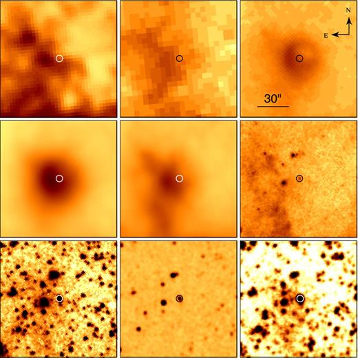
From left to right, and from top to bottom: Herschel PACS 160 μm, Spitzer MIPS 70 and 24 μm, WISE 22 and 12 μm, Spitzer IRAC 8 and 3.6 μm, 2MASS J-band and DSS-II red-band images of the region of the LMC containing the new circular shell and its central star (indicated by a circle). The orientation and the scale of the images are the same. At the distance of the LMC of 50 kpc, 30 arcsec corresponds to ≈7.2 pc.
The central star is offset by several arcsec from the geometric centre of the shell being closer to its brightest portion. This displacement and the brightness asymmetry could be understood if the shell impinges on a more dense ambient medium in the eastern direction. The presence of the dense material on the eastern side of the shell could be inferred from all but the J-band images, showing a diffuse emission to the east of the star (see also Section 6). This region is classified in Bica et al. (1999) as ‘NA’, i.e. a stellar system clearly related to emission (named in the SIMBAD data base as BSDL 161). Alternatively, the enhanced brightness of the eastern side of the shell and the displacement of the star might be caused by the stellar motion in the west–east direction (we discuss both possibilities in Section 7).
The g′-band acquisition image obtained during our spectroscopic follow-up with the Gemini Multi-Object Spectrograph (GMOS; Hook et al. 2004) resolved the central star into two components (hereafter star 1 and star 2; marked in Fig. 2 by a large and small white circle, respectively) separated from each other by ≈2 arcsec or ≈0.5 pc in projection. Using the VizieR catalogue access tool,5 we searched for photometry of these stars and found four catalogues which provide their UBV (Braun 2001), UBVI (Zaritsky et al. 2004), JHKs (Kato et al. 2007) and IRAC band (SAGE LMC and SMC6 IRAC Source Catalog7) magnitudes separately. Interestingly, the JHKs survey of the Magellanic Clouds by Kato et al. (2007)8 resolved star 1 into two components separated from each other by 1 arcsec or ≈0.24 pc in projection. For the brightest of these two stars, we keep the name star 1, while the second one, shown in Fig. 2 by a green diamond, we call star 3. The details of the three stars are summarized in Table 1. A possible relationship between these stars is discussed in Section 7.
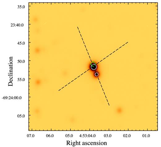
GMOS g′-band acquisition image of the central star of the circular shell showing that it is composed of two components, separated from each other by ≈2 arcsec or ≈0.5 pc in projection. The new WR star BAT99 3a (star 1) is marked by a large circle. A small circle marks star 2 (B0 V). A diamond indicates the position of a third star (star 3), revealed by the JHKs survey of the Magellanic Clouds by Kato et al. (2007). The orientations of the spectrograph slit in our two Gemini observations are shown by dashed lines. See the text for details.
Details of three stars in the centre of the circular shell. The spectral types, SpT, of stars 1 (BAT99 3a) and 2 are based on our spectroscopic observations, while that of star 3 is inferred from the JHKs photometry (see the text for details) and therefore should be considered with caution. The UBVI photometry is from Zaritsky et al. (2004). The coordinates and JHKs photometry are from Kato et al. (2007). The IRAC photometry is from the SAGE LMC and SMC IRAC Source Catalog.
| star 1 | star 2 | star 3 | |
|---|---|---|---|
| SpT | WN3b+O6 V | B0 V | O8.5 V (?) |
| α (J2000) | |$04^{\rm h} 53^{\rm m} 03{^{s}_{.}}76$| | |$04^{\rm h} 53^{\rm m} 03{^{s}_{.}}60$| | |$04^{\rm h} 53^{\rm m} 03{^{s}_{.}}86$| |
| δ (J2000) | −69°23′51|${^{\prime\prime}_{.}}$|8 | −69°23′53|${^{\prime\prime}_{.}}$|8 | −69°23′50|${^{\prime\prime}_{.}}$|9 |
| U (mag) | 13.167 ± 0.041 | 14.502 ± 0.058 | – |
| B (mag) | 14.210 ± 0.035 | 15.255 ± 0.044 | – |
| V (mag) | 14.391 ± 0.099 | 15.298 ± 0.231 | – |
| I (mag) | 14.402 ± 0.102 | 15.441 ± 0.046 | – |
| J (mag) | 14.630 ± 0.010 | 15.550 ± 0.020 | 16.420 ± 0.040 |
| H (mag) | 14.530 ± 0.040 | 15.600 ± 0.020 | 15.920 ± 0.030 |
| Ks (mag) | 14.610 ± 0.040 | 15.620 ± 0.050 | 15.670 ± 0.070 |
| [3.6] (mag) | 14.053 ± 0.052 | 15.311 ± 0.086 | – |
| [4.5] (mag) | 14.120 ± 0.047 | 15.377 ± 0.077 | – |
| [5.8] (mag) | 13.764 ± 0.069 | – | – |
| [8.0] (mag) | 13.439 ± 0.100 | – | – |
3 SPECTROSCOPIC FOLLOW-UP WITH GEMINI-SOUTH
3.1 Observations and data reduction
To determine the spectral type of the central star associated with the 24-μm circular shell, we used the Poor Weather time at Gemini-South under the programme-ID GS-2011A-Q-88. The spectroscopic follow-up was performed with the GMOS in a long-slit mode with a slit width of 0.75 arcsec. Two spectra were collected on 2011 February 9 and March 5. The log of these and five subsequent observations with the du Pont telescope and the SALT (see Section 4) is listed in Table 2.
Journal of the observations.
| Spectrograph | Date | Grating | Spectral scale | Spatial scale | Slit | Slit PA | Spectral range |
|---|---|---|---|---|---|---|---|
| (l mm−1) | ( Å pixel−1) | (arcsec pixel−1) | arcsec | (°) | (Å) | ||
| GMOS (Gemini) | 2011 February 9 | 600 | 0.46 | 0.073 | 0.75 | 125 | 3800–6750 |
| GMOS (Gemini) | 2011 March 5 | 600 | 0.46 | 0.073 | 0.75 | 22 | 3800–6750 |
| B&C (du Pont) | 2012 December 6 | 1200 | 0.79 | 0.70 | 1.00 | 90 | 3815–5440 |
| B&C (du Pont) | 2012 December 13 | 1200 | 0.79 | 0.70 | 1.00 | 90 | 3815–5440 |
| B&C (du Pont) | 2012 December 28 | 1200 | 0.79 | 0.70 | 1.00 | 25 | 3815–5440 |
| RSS (SALT) | 2013 January 26 | 900 | 0.99 | 0.25 | 1.25 × 480 | 130 | 3580–6700 |
| RSS (SALT) | 2013 January 28 | 900 | 0.98 | 0.25 | 1.25 × 480 | 130 | 4170–7300 |
The acquisition image obtained during the first observation resolved the central star into two components, and the decision was made then by the observer to put only the brightest star (star 1; see Table 1) in the slit [with a position angle (PA) of PA = 125°, measured from north to east; see Fig. 2]. A quick extraction of the spectrum allowed us to classify this star as a WN3 star with absorption lines (see Section 3.2.1); hence, we decided to re-observe it to search for shifts in the radial velocity (RV) as a result of possible binarity. The second spectrum was taken with the slit aligned along stars 1 and 2 (PA = 22°).
The first spectrum was obtained under fairly good conditions: with only some clouds and an ≈1 arcsec seeing. The aimed signal-to-noise ratio (S/N) of ≈200 was achieved with a total exposure time of 450 s. For the second observation, in order to get fairly good S/N on the fainter star (star 2), we preferred to double the exposure time, which resulted in the S/N of 350 in the spectrum of star 1. Calibration-lamp (CuAr) spectra and flat-field frames were provided by the Gemini Facility Calibration Unit.
The bias subtraction, flat-fielding, wavelength calibration and sky subtraction were executed with the gmos package in the gemini library of the iraf9 software. In order to fill the gaps between GMOS-S's EEV CCDs, each observation was divided into three exposures obtained with a different central wavelength, i.e. with a 5 Å shift between each exposure. The extracted spectra were obtained by averaging the three individual exposures, using a sigma clipping algorithm to eliminate the effects of cosmic rays. The B600 grating was used to cover the spectral range λλ = 3800–6750 Å with a reciprocal dispersion of ≈0.5 Åpixel−1 and the average spectral resolution full width at half-maximum (FWHM) of ≈4.08 Å. The accuracy of the wavelength calibration estimated by measuring the wavelength of 10 lamp emission lines is 0.065 Å. A spectrum of the white dwarf LTT 3218 was used for flux calibration and removing the instrument response. The resulting spectra of stars 1 and 2 are shown in Figs 3 and 4, respectively.
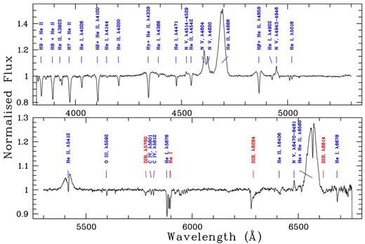
Normalized spectrum of the new WR star BAT99 3a (star 1) in the LMC observed with Gemini-South on 2011 March 5 with principal lines and most prominent DIBs indicated.

Normalized spectrum of star 2 (B0 V) observed with Gemini-South with principal lines and most prominent DIBs indicated.
Note that star 1 and the standard star were observed at different air masses, during different nights, and were not observed with the long slit aligned with the parallactic angle. These make the absolute flux calibration of the Gemini spectra very uncertain.
Equivalent widths (EWs), FWHMs and heliocentric RVs of main lines in the spectra of stars 1 and 2 (measured applying the midas programs; see Kniazev et al. 2004 for details) are summarized in Tables 3 and 4, respectively. All wavelengths are in air. For EWs and RVs, we give their mean values derived from both spectra, while for measurements of FWHMs, we used the second spectrum alone owing to its better quality.
EWs, FWHMs and RVs of main lines in the spectrum of the new WR star BAT99 3a (star 1). For EWs and RVs, we give their mean values derived from both Gemini spectra, while for measurements of FWHMs, we used the second spectrum alone owing to its better quality.
| λ0(Å) Ion | EW(λ)a | FWHM(λ)a | RV |
|---|---|---|---|
| (Å) | (Å) | ( km s−1) | |
| 3889 He ii + H8 | 1.35 ± 0.13 | 7.37 ± 0.16 | 311 ± 40 |
| 3968 He ii + H7 | 1.73 ± 0.17 | 8.32 ± 0.11 | 271 ± 11 |
| 4026 He ii | 0.56 ± 0.11 | 5.88 ± 0.15 | 353 ± 8 |
| 4100 He ii + Hδ | 1.67 ± 0.16 | 8.09 ± 0.14 | 285 ± 6 |
| 4144 He i | 0.05 ± 0.03 | 4.86 ± 0.35 | 307 ± 50 |
| 4200 He ii | 0.47 ± 0.11 | 5.82 ± 0.12 | 317 ± 8 |
| 4339 He ii + Hγ | 1.49 ± 0.15 | 7.81 ± 0.11 | 268 ± 6 |
| 4388 He i | 0.14 ± 0.09 | 5.08 ± 0.35 | 361 ± 35 |
| 4471 He i | 0.35 ± 0.08 | 4.12 ± 0.11 | 315 ± 6 |
| 4542 He ii | 0.62 ± 0.12 | 6.81 ± 0.18 | 266 ± 8 |
| 4604 N v | −2.50 ± 0.28 | 13.73 ± 0.51 | 192 ± 8 |
| 4620 N v | −1.50 ± 0.20 | 10.50 ± 2.00 | 219 ± 11 |
| 4686 He ii | 0.02 ± 0.03* | 3.28 ± 0.21* | 282 ± 25 |
| 4686 He ii | −16.37 ± 0.68* | 31.10 ± 0.21* | 280 ± 15 |
| 4859 He ii + Hβ | 1.14 ± 0.14* | 7.09 ± 0.15* | 244 ± 10 |
| 4859 He ii + Hβ | −1.52 ± 0.52* | 28.87 ± 4.09* | 146 ± 50 |
| 4922 He i | 0.11 ± 0.06 | 3.43 ± 0.28 | 306 ± 20 |
| 4944 N v | −0.50 ± 0.13 | 8.77 ± 0.43 | 175 ± 21 |
| 5412 He ii | 0.26 ± 0.07* | 5.36 ± 0.26* | 261 ± 10 |
| 5412 He ii | −2.41 ± 0.83* | 54.91 ± 2.10* | 270 ± 14 |
| 5592 O iii | 0.11 ± 0.05 | 4.40 ± 0.21 | 305 ± 14 |
| 5876 He i | 0.50 ± 0.07 | 4.64 ± 0.10 | 313 ± 21 |
| 6560 He ii + Hα | 0.56 ± 0.07* | 5.08 ± 0.15* | 211 ± 20 |
| 6563 He ii + Hα | −12.66 ± 0.86* | 47.58 ± 0.79* | 177 ± 15 |
| 6678 He i | 0.17 ± 0.05 | 4.66 ± 0.30 | 302 ± 9 |
aNote that some of the starred EWs and FWHMs are significantly affected because of the binary nature of BAT99 3a. The negative (positive) EWs correspond to emission (absorption) lines originating from the WR (O) component of BAT99 3a (see the text for details).
EWs, FWHMs and RVs of main lines in the spectrum of star 2 (B0 V).
| λ0(Å) Ion | EW(λ) | FWHM(λ) | RV |
|---|---|---|---|
| (Å) | (Å) | ( km s−1) | |
| 3889 He i + H8 | 1.03 ± 0.01 | 7.84 ± 0.08 | 298 ± 1 |
| 3968 He i + H7 | 3.95 ± 0.08 | 10.14 ± 0.22 | 461 ± 6 |
| 4026 He i | 1.00 ± 0.02 | 4.78 ± 0.07 | 273 ± 1 |
| 4102 Hδ | 3.71 ± 0.10 | 10.18 ± 0.30 | 288 ± 7 |
| 4144 He i | 0.55 ± 0.02 | 4.52 ± 0.13 | 283 ± 1 |
| 4340 Hγ | 3.71 ± 0.09 | 10.76 ± 0.29 | 290 ± 6 |
| 4388 He i | 0.52 ± 0.01 | 4.28 ± 0.06 | 274 ± 1 |
| 4471 He i | 1.07 ± 0.03 | 5.53 ± 0.15 | 243 ± 2 |
| 4553 Si iii | 0.12 ± 0.01 | 3.79 ± 0.22 | 262 ± 1 |
| 4861 Hβ | 3.42 ± 0.06 | 9.75 ± 0.20 | 257 ± 4 |
| 4922 He i | 0.68 ± 0.01 | 4.62 ± 0.08 | 258 ± 1 |
| 5740 Si iii | 0.08 ± 0.01 | 4.15 ± 0.32 | 231 ± 1 |
| 5876 He i | 0.71 ± 0.02 | 4.82 ± 0.10 | 263 ± 1 |
| 6563 Hα | 2.68 ± 0.09 | 7.70 ± 0.28 | 250 ± 4 |
| 6678 He i | 0.18 ± 0.01 | 4.14 ± 0.06 | 238 ± 4 |
3.2 Spectral classification
3.2.1 Star 1: a new WR star in the LMC
The spectrum of star 1 (see Fig. 3) is dominated by strong emission lines of Hα, He ii λ4686 and N v λλ4604, 4620. The Hα and He ii λ4686 lines show central absorption reversals. Several weaker emissions of N v (at λλ4514-4529, 4943-4946 and 6470–6481) are also detected. There are also several lower intensity broad emission features with narrow absorption reversals, of which the most prominent are Hβ+He ii λ4859 and He ii λ5412. None of the emission lines shows P Cygni profiles. Other H, He i and He ii lines are almost purely in absorption. The O iii λ5592 and C iv λλ5801, 5812 lines are also purely in absorption. The low interstellar extinction in the direction towards the LMC is manifested in several weak diffuse interstellar bands (DIBs). A prominent absorption visible in the spectrum at 6277 Å is telluric in origin.
The presence of the N v λλ4604, 4620 emission lines and the absence of the N iv λ4057 one imply that the emission spectrum belongs to a WR star of the ionization subclass WN3 (Smith, Shara & Moffat 1996). The FWHM of the He ii λ4686 (emission) line of 31.1 ± 0.21 Å slightly exceeds the empirically determined limit of 30 Å for broad-lined stars (Smith et al. 1996), which implies that star 1 can be classified WN3b. Since it is believed that broad-lined WR stars are true hydrogen-free WN stars (Smith & Maeder 1998; cf. Foellmi, Moffat & Guerrero 2003), one can assume that the numerous absorption lines in the spectrum of star 1 are due to a second (unresolved) star, either a binary companion or a separate star located on the same line of sight. Our subsequent spectroscopic observations of star 1 showed that it is a binary system (see Section 4). We name star 1 BAT99 3a using the numbering system based on extending the Breysacher, Azzopardi & Testor (1999) catalogue, as suggested by Howarth & Walborn (2012).
An indirect support to the possibility that the spectrum of BAT99 3a is a superposition of two spectra comes from the position of this star on the plot of EW(5412) versus FWHM(4686) for WN stars in the LMC (see fig. 14 of Smith et al. 1996), where it lies in a region occupied by binary and composite stars.
Detailed comparison of the two Gemini spectra of BAT99 3a taken 24 d apart did not show evidence of significant change in RVs typical of close binaries. Although this might imply that the WR and O stars are unrelated to each of the other members of the same (unrecognized) star cluster (cf. Section 7), our subsequent spectroscopic observations (see Section 4) showed that the two stars form a binary system. Moreover, we know that the Gemini spectra were taken outside of the periastron passage and hence should not show significant RV variability.
3.2.2 Star 2
The spectrum of star 2 is dominated by H and He i absorption lines (see Fig. 4). No He ii lines are visible in the spectrum, which implies that star 2 is of B type. Using the EW(Hγ)–absolute magnitude calibration by Balona & Crampton (1974) and the measured EW(Hγ) = 3.71 ± 0.09 Å, we estimated the spectral type of this star as B0 V. The same spectral type also follows from equation (1). With EW(4922) = 0.68 ± 0.01 Å, we found SpT ≈ 10, which corresponds to B0 V stars (Kerton et al. 1999).
Using the B and V magnitudes of star 2 from Table 1 and intrinsic (B − V)0 colour of −0.26 mag (typical of B0 V stars; e.g. Martins & Plez 2006), and assuming the standard total-to-selective absorption ratio RV = 3.1 (cf. Howarth 1983), we found the visual extinction, AV, towards this star and its absolute visual magnitude, MV, of ≈0.67 and −3.87 mag, respectively. The latter estimate agrees well with MV of B0 V stars of −3.84 mag, derived by extrapolation from the absolute magnitude calibration of Galactic O stars of Martins & Plez (2006).
4 ADDITIONAL SPECTROSCOPIC OBSERVATIONS WITH THE du pont TELESCOPE AND THE SALT
To clarify the possible binary status of BAT99 3a, five additional spectra were taken in 2012 December–2013 January.
Three spectra were observed as time fillers at the du Pont 2.5-m telescope (Las Campanas, Chile) on 2012 December 6, 13 and 28, using the B&C spectrograph with a slit width of 1 arcsec. An S/N of ≈130 was obtained after a 1 h exposure each time. The wavelength calibration was done using spectra of an HeAr lamp. The full spectral range is λλ3815–5440 Å, the average wavelength resolution is ≈0.8 Åpixel−1 (FWHM ≈ 2.44 Å) and the accuracy of the wavelength of 10 lamp emission lines is 0.055 Å. No spectrophotometric standard was observed to calibrate the spectra in flux.
Two other spectra were taken with the SALT (Buckley, Swart & Meiring 2006; O'Donoghue et al. 2006) on 2013 January 26 and 28, using the Robert Stobie Spectrograph (RSS; Burgh et al. 2003; Kobulnicky et al. 2003) in the long-slit mode. The RSS pixel scale is 0.127 arcsec and the effective field of view is 8 arcmin in diameter. We utilized a binning factor of 2, to give a final spatial sampling of 0.254 arcsec pixel−1. As indicated in Table 2, the volume phase holographic grating GR900 was used mainly to cover the spectral ranges 3580–6700 Å and 4170–7300 Å with a final reciprocal dispersion of ∼0.98 Å pixel−1 and spectral resolution FWHM of 4–5 Å. Observations were done with exposure times of 20 min for the blue spectral range and 10 min for the red one. Unfortunately, they were carried out close to the twilight time and under the very poor weather conditions. Spectra of Ar comparison arcs were obtained to calibrate the wavelength scale. Spectrophotometric standard star LTT 4364 was observed for the relative flux calibration. Primary reduction of the data was done with the SALT science pipeline (Crawford et al. 2010). After that, the bias- and gain-corrected and mosaicked long-slit data were reduced in the way described in Kniazev et al. (2008b). We note that SALT is a telescope with a variable pupil, so that the illuminating beam changes continuously during the observations. This makes the absolute flux/magnitude calibration impossible, even using spectrophotometric standard stars or photometric standards. At the same time, the final relative flux distribution is very accurate and does not depend on the PA because SALT has an atmospheric dispersion corrector (O'Donoghue 2002).
Special care was taken for normalizing the continuum of all seven spectra. The method consists of normalizing all spectra with respect to a reference spectrum before we fit the continuum on the overall mean spectrum. The spectrum with the best S/N is always chosen as the reference. All the other spectra are divided by the reference, and the results of the divisions are fitted using a Legendre polynomial of the fourth order. All individual spectra are divided by the respective fits, so their continuum has the same shape as the reference spectrum. In our case, we took the second spectrum from Gemini as the reference. The continuum on the overall mean spectrum was fitted with a Legendre polynomial of the eighth order and applied to all spectra normalized to the reference spectrum.
The top left-hand panel of Fig. 5 shows a montage of the residuals of the Gemini and du Pont spectra subtracted by the normalized average spectrum. The spectra are organized in chronological order, and the time (HJD−2455550) is indicated for each spectrum. The du Pont spectra are used to show the line variations near the periastron passage (see below), and the Gemini ones are used as a reference when the orbital motion is small. The residuals show that all absorption and emission lines are varying with time. The S shape of the residuals at the same wavelength as the spectral lines is the sign of RV variations. The bottom left-hand panel shows the square root of the Temporal Variance Spectrum (TVS; Fullerton, Gies & Bolton 1996). The spectrum is significantly variable at the wavelength where the corresponding TVS1/2 value is over the threshold plotted with a dashed line. We find that all the emission (WR) lines show a double peak in the TVS, as expected for RV motions.
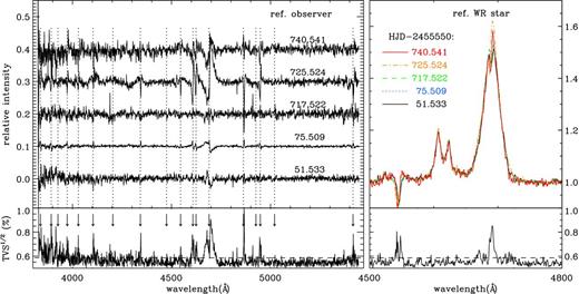
Left: the top panel shows a montage of the residuals (individual spectra minus mean) for our Gemini and du Pont observations in the observer's reference frame. HJD−2455550 is indicated for each residual, and selected spectral lines are marked with a dotted line. The bottom panel shows the TVS, which shows broad double-peaked profiles associated with the emission lines, and narrow peaks associated with the absorption lines. Right: the top panel shows the superposition of the five spectra placed in the reference frame of the WR star. The TVS (bottom panel) shows only signatures of the motion of the absorption lines (with respect to the emission ones) and a change in amplitude of the He ii lines.
To analyse the RV variability, we used all seven spectra. The RVs for each line were determined by a non-linear fit of their profile. Only the He ii λλ4686, 4859 emission lines were not fitted, since they are broad, their profiles are varying in amplitude and they are blended with absorption lines. We assume that all the line profiles are close enough to a Voigt function, even the two N v emission lines at 4604 and 4620 Å, for which we get a good fit. The results are listed in Table 5 and plotted in Fig. 6. We averaged the RV values for each line series; the absorption Balmer and He ii lines are plotted with diamonds and triangles, respectively, and the (red) squares are the RVs for the two Nv emission lines. The dashed lines are the scatter in RV of the Balmer lines in the spectrum of star 2, as observed simultaneously with the second spectrum of BAT99 3a at Gemini. The error bars are assumed to be the rms of the individually measured RVs within a line type (note that our spectral range includes five Balmer and four He ii lines well observed). We prefer to plot the RVs of the N v lines without the errors, since only two lines were observed with sufficient S/N.
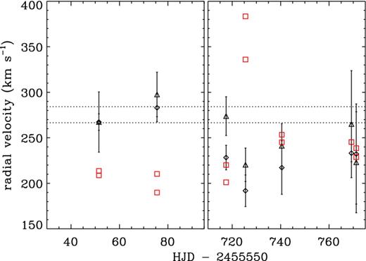
RV changes with time in the spectrum of BAT99 3a. The average RVs for the Balmer and He ii absorption lines are plotted with (black) diamonds and triangles, respectively. The (red) squares are the RVs for the N v λλ4604, 4620 emission lines. The dashed lines are the scatter in RV of the Balmer lines in star 2, as observed in the second Gemini spectrum.
Mean RVs of N v λλ4604, 4640 emission lines (associated with the WR star) and of the Balmer and He ii absorption lines (associated with the O companion star) for seven observations of BAT99 3a.
| HJD | RV(N v) | RV(Balmer) | RV(He ii) |
|---|---|---|---|
| ( km s−1) | ( km s−1) | ( km s−1) | |
| 2455601.533 | 211 ± 5 | 267 ± 18 | 267 ± 66 |
| 2455625.509 | 200 ± 20 | 283 ± 31 | 298 ± 49 |
| 2456267.522 | 211 ± 19 | 228 ± 13 | 273 ± 21 |
| 2456275.524 | 360 ± 47 | 192 ± 17 | 220 ± 18 |
| 2456290.541 | 249 ± 8 | 217 ± 29 | 241 ± 24 |
| 2456319.300 | 245 ± 20 | 233 ± 9 | 265 ± 59 |
| 2456321.301 | 242 ± 10 | 232 ± 40 | 233 ± 55 |
In the top-right panel of Fig. 5, the observed spectra are placed into the reference frame of the emission lines (i.e. the WR star). We see that the He ii λ4686 line intensity increases near periastron passage. In the TVS, shown at the bottom-right panel of Fig. 5, we see a significant peak centred on 4686 Å. Its blue side is dominated by the motion of the O star absorption line, but the red one shows a variable emission excess, which could be attributed to the emission of a wind–wind collision zone. Unfortunately, the absorption lines blended with the He ii emission lines make this attribution ambiguous.
The additional spectroscopic observations allow us to confirm that BAT99 3a is a binary system, and that the absorption lines originate in a massive O companion, not in the WR star itself. The RV variations show that the binary is close and eccentric, and that we had the chance to observe it near the periastron passage in 2012 December. Our seven spectra, however, are not sufficient to determine the orbital parameters of the system.
We searched for possible photometric variability of BAT99 3a using the Massive astrophysical compact halo object project photometric data base (Alcock et al. 1999), but none was found. The presence of the O-type companion to the WR star implies that this system could be a source of X-ray emission, arising from colliding stellar winds (e.g. Usov 1992). Unfortunately, the part of the LMC containing the circular shell was not observed with modern X-ray telescopes.
Since the majority of massive stars form close binary systems (e.g. Chini et al. 2012; Sana et al. 2012, 2013), one can suspect that star 2 could be a binary as well. The bad seeing during the third observation at du Pont, however, did not allow us to reliably measure RVs for this star and compare them with those measured in the Gemini spectrum.
5 BAT99 3A: SPECTRAL ANALYSIS AND STELLAR PARAMETERS
The spectral analysis was performed using the state-of-the-art non-LTE powr code. powr is a model atmosphere code especially suitable for hot stars with expanding atmospheres. The code solves the radiative transfer and rate equations in the comoving frame, calculates non-LTE population numbers and delivers a synthetic spectrum in the observer's frame.11 The pre-specified wind velocity field takes the form of a β-law in the supersonic region. In the subsonic region, the velocity field is defined such that a hydrostatic density stratification is obtained. A closer description of the assumptions and methods used in the code is given by Gräfener, Koesterke & Hamann (2002) and Hamann & Gräfener (2004). The so-called microclumping approach is used to account for wind homogeneities. The density contrast between a clumped and a smooth wind with an identical mass-loss rate is described by the clumping factor D (cf. Hamann & Koesterke 1998). Line blanketing is treated using the superlevel approach (Gräfener et al. 2002), as originally introduced by Anderson (1989). We adopt β = 1 for the exponent in the β-law. The clumping factor D is set to 10 for the WR star and to unity for the O star.
The model parameters are determined by iteratively fitting the spectral energy distribution (SED) and synthetic normalized spectrum to the observations (see Figs 7 and 8, respectively). The synthetic composite spectrum used for BAT99 3a is the sum of two models corresponding to its two components, weighted according to their relative contribution to the overall flux. The temperatures are obtained from the line ratios of different ions, while the mass-loss rate of the WR component is derived from the strengths of emission lines. The effective gravity log geff of the O companion is inferred from the wings of prominent hydrogen lines. The total luminosity L1 + L2 is determined from the observed SED, while the light ratio is obtained from the normalized spectrum. In our case, the effect of the light ratio is most easily isolated from the other parameters by simultaneously inspecting lines which clearly originate in one of the components, e.g. He i lines belonging to the O component, or N v and He ii emission lines from the WR component. Once the light ratio and total luminosity are known, the individual luminosities follow.
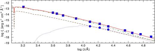
Reddened synthetic SEDs of the WR (brown dashed line) and O (green dot–dashed line) components of BAT99 3a, star 3 (purple dotted line) and BAT99 3a + star 3 (red solid line). Blue squares denote the total photometry of BAT99 3a and star 3, while blue circles denote the photometry of star 3 alone.
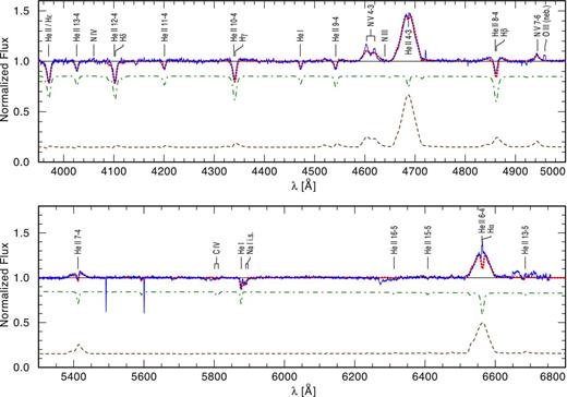
Normalized synthetic spectra of the WR (brown dashed line) and O (green dot–dashed line) components of BAT99 3a, as well as of BAT99 3a + star 3 (red dotted line). The component spectra are weighted according to their relative contributions to the combined flux. Star 3 hardly contributes to the flux and is therefore not included. The normalized observed spectrum, taken at Gemini on 2011 February 9, is also shown (blue solid line).
Fig. 7 plots the synthetic SEDs of the best-fitting models for both components of BAT99 3a as well as for star 3. The total synthetic SED belonging to BAT99 3a and star 3 (red solid line) is also plotted. The blue squares denote the total far-ultraviolet (FUV) (Parker et al. 1998), UBVI (Zaritsky et al. 2004), JHKs (Kato et al. 2007) and IRAC photometry of BAT99 3a and star 3. The FUV magnitude also includes a contribution from the nearby B star (star 2). This contribution, however, is insignificant because of the spectral type of the star. On the other hand, star 2 might somewhat influence the IRAC 5.8 and 8 μm photometry, which is indeed implied by the small observed IR excess compared to the synthetic SED in Fig. 7. Since the JHKs survey by Kato et al. (2007) resolves BAT99 3a and star 3, we denote the JHKs magnitudes corresponding to star 3 only (blue circles) as well. The corresponding normalized spectra of the different components are shown in Fig. 8. The contribution of star 3 is negligible and therefore not shown. The sum of all model spectra (red dotted line) is further compared with the Gemini spectrum observed on 2011 February 9 (blue solid line).
The stellar parameters and abundances used for the best-fitting WR and O star models are compiled in Table 6, where we also provide the number of ionizing photons per second for hydrogen (Q0), He i (Q1) and He ii (Q2). For the O star, we also give the gravity, log g, and a projected rotational velocity, vsin i. The absolute visual magnitudes inferred for the binary components imply a V-band magnitude difference of ΔV = 1.89 mag, i.e. the O component contributes ≈5.7 times more than the WR component in the visual band. The H and N abundances for the WR star are derived from the spectral analysis. The adopted abundances of the remaining elements, which cannot be derived from the available spectra, are based on a recent work by Hainich et al. (2014). For the O component, we adopt typical LMC abundances (Hunter et al. 2007; Trundle et al. 2007).
Stellar parameters for the WN3 and O-type components of BAT99 3a.
| WN3 | O6 V | |
|---|---|---|
| T* (kK) | 89 | 38 |
| log Rt ( Rȯ) | 1.0 | – |
| log g (cm s−2) | – | 3.73 |
| log geff (cm s−2) | – | 3.60 |
| log L ( Lȯ) | 5.45 | 5.20 |
| v∞ ( km s−1) | 1800 | 2500 |
| D | 10 | 1 |
| R*( Rȯ) | 2.23 | 9.20 |
| |$\log \skew4\dot{M}$| ( Mȯ yr− 1) | −5.8 | −7.0 |
| log Q0 (s−1) | 49.4 | 48.82 |
| log Q1 (s−1) | 49.2 | 47.79 |
| log Q2 (s−1) | 46.2 | 42.31 |
| vsin i (km s−1) | – | 80 |
| E(B − V) (mag) | 0.18 | 0.18 |
| AV (mag) | 0.56 | 0.56 |
| RV | 3.1 | 3.1 |
| MV (mag) | −2.86 | −4.75 |
| H (mass fraction) | 0.20 | 0.73 |
| He (mass fraction) | 0.80 | 0.27 |
| C (mass fraction) | 0.7 × 10⁻⁴ | 4.7 × 10⁻⁴ |
| N (mass fraction) | 0.008 | 7.8 × 10⁻⁵ |
| Fe (mass fraction) | 7.0 × 10⁻⁴ | 7.0 × 10⁻⁴ |
For the WR component, we also estimate the initial mass, Mi, and age of ≈30 Mȯ and ≈7 Myr, respectively, using the single star evolutionary tracks from Meynet & Maeder (2005). To estimate the current mass of the WR component, Mcur, we make use of the mass–luminosity relation for homogenous WR stars (Gräfener et al. 2011; see their equation 11), which is dependent on the hydrogen abundance. If the WR star is indeed homogenous, e.g. because it is a rapid rotator (Heger & Langer 2000), our analysis implies a hydrogen abundance in the stellar core of ≈0.2, and the resulting Mcur is 23 Mȯ. More likely, however, the core is almost depleted of hydrogen, which would imply that Mcur is 14 Mȯ. Since rotational velocities of WR stars are poorly understood at present and were claimed to be indirectly observed only in a few WR stars (Chené & St-Louis 2005; Shenar, Hamann & Todt 2014), we may merely conclude that Mcur lies somewhere between these two extremes. The relatively large RV amplitude of the WR component in comparison with the primary O star (see Table 5 and Fig. 6), however, suggests a value closer to 14 Mȯ than to 23 Mȯ.
On the other hand, the single star evolutionary tracks from Köhler et al. (in preparation)12 give for the O star an initial mass and age of ≈30 Mȯ and ≈3 Myr, respectively. The latter figure is much smaller than the estimated age of the WR star of 7 Myr, which implies that there was mass transfer in the binary system and that the O star is a rejuvenated mass gainer (e.g. Schneider et al. 2014), and that Mi of the WR star cannot be estimated from single star models. For Mcur = 14 Mȯ, one can expect that Mi of the WR star was about 40 Mȯ (Wellstein & Langer 1999), which would imply an age of this star of ≈6 Myr. What is unexpected in the above consideration is to have a large eccentricity of the binary system after the mass transfer. This could, however, be understood if the system was kicked out of the parent star cluster (after the mass transfer was completed) either because of dynamical encounter with another massive (binary) system or due to dissolution of a multiple system (cf. Section 7).
While it is not possible to quantify the detailed stellar parameters of star 3 with the current data, the photometric data imply that this star is highly reddened. With no indications for a later-type star in the available spectrum, we conclude that star 3 is of O or B type. In Fig. 7, we illustrate that the observed photometry is consistent with the SED typical of an O8.5 V star with an adopted colour excess E(B − V) = 1.75 mag (cf. Section 7).
Since the O component of BAT99 3a does not show clear evidence for wind lines in the available spectra, a spectroscopic calculation of its v∞ and |$\skew4\dot{M}$| is not possible. Nevertheless, |$\skew4\dot{M}$| can be constrained because larger values would lead to observable effects on the spectrum. The value of |$\skew4\dot{M}$| given in Table 6 for the O component should therefore be considered as an upper limit. As no information regarding v∞ of the O component is available from its spectrum, we merely adopt a value typical of stars of similar spectral type (see Table 6), based on the work by Mokiem et al. (2007).
For the Galactic interstellar reddening, we adopt a colour excess of E(B − V) = 0.03 mag. To model the LMC interstellar reddening, we assume the reddening law suggested by Howarth (1983) with RV = 3.1. The best fit to the whole SED was achieved with E(B − V) = 0.18 mag, which is comparable to that of 0.22 mag derived for star 2 in Section 3.2.2. On the other hand, a similar fit to the SED could also be obtained with a colour excess of 0.12 mag if the luminosities of the two companions are both reduced by 0.1 dex. This E(B − V) is closer to the one obtained from the analysis of the circular shell (see Section 6). Future UV observations should enable a much more precise determination of the luminosities and redenning.
A comparison of the stellar parameters of the WR component with the almost complete sample of the WR stars in the LMC (Hainich et al. 2014) reveals that the analysed WR star is one of the hottest WR stars in the LMC. While Q0 and Q1 of the WR component are comparable to those of its O companion, the number of He ii ionizing photons is four orders of magnitude larger, placing BAT99 3a among the strongest He ii ionizing sources in the LMC. This is in very good agreement with the unique signature of He ii emission observed in the circular shell, as discussed in Section 6.
6 CIRCULAR SHELL
6.1 Circular shells around WR stars
Johnson & Hogg (1965) were the first who noted association of WR stars with filamentary shells and suggested that they are the result of interaction between the material ejected from the stars and the interstellar matter (cf. Avedisova 1972). This suggestion was further elaborated to take into account the interaction of the WR wind with the circumstellar material shed during the preceding red supergiant or LBV stages (e.g. D'Ercole 1992; García-Segura, Langer & Mac Low 1996a,b; Brighenti & D'Ercole 1997). The circumstellar shells produced in this process show signatures of CNO-processing (e.g. Esteban et al. 1992; Stock, Barlow & Wesson 2011) and are associated exclusively with WNL stars (e.g. Chu 1981; Lozinskaya & Tutukov 1981; Gruendl et al. 2000; Gvaramadze et al. 2010c), i.e. the very young WR stars, whose winds are still confined within the region occupied by the circumstellar material or only recently emerged from it (Gvaramadze et al. 2009; Burgemeister et al. 2013). The size and crossing time of this region determine the characteristic size and lifetime of the circumstellar shells, which are typically several pc and several tens of thousands of years, respectively. The winds of more evolved (WNE) WR stars interact directly with the local interstellar medium and create new, generally more extended shells. Correspondingly, the chemical composition of these interstellar shells is similar to that of ordinary H ii regions (e.g. Esteban et al. 1992; Stock et al. 2011).
Since the WR component of BAT99 3a is of WNE type, it is natural to expect that its associated shell should consist mostly of interstellar matter. In Section 6.3, we support this expectation by an analysis of the long-slit spectra of the shell obtained with the Gemini and du Pont telescopes and the SALT.
6.2 Hα imaging of the shell
Before discussing the long-slit spectra, we present an Hα image of the shell obtained as part of the Magellanic Clouds Emission Line Survey 2 (MCELS2; PI: Y.-H. Chu). This survey used the MOSAIC ii camera on the Blanco 4-m telescope at the Cerro Tololo Inter-American Observatory (Muller et al. 1998) to image the entire LMC and SMC in the Hα line only. The region of the LMC containing the shell was observed on 2008 December 12 with three dithered 300 s exposures, through a 80 Å bandwidth filter centred at 6563 Å. The image was overscan, crosstalk, bias and flat-field corrected using standard routines in iraf. An astrometric solution and distortion correction were obtained by comparison to 2MASS Point Source Catalog (Skrutskie et al. 2006), and have a typical accuracy of ≈150 mas.
The Hα image of the shell is presented in Fig. 9. The shell appears as an incomplete circle bounded on the eastern side by two concentric arc-like filaments, separated from each other by ≈4 arcsec (or ≈1 pc), and on the northern side by a thick amorphous arc. There is no distinct limb-brightened emission in the south-west direction, but the shell can still be discerned because of a diffuse emission filling its interior. BAT99 3a and star 2 are clearly resolved in the image. The lopsided appearance of the shell and the off-centred position of the stars suggest that the ambient medium is denser in the eastern direction, which is consistent with the presence of a prominent H ii region in this direction (cf. Section 2 and see also the next section).
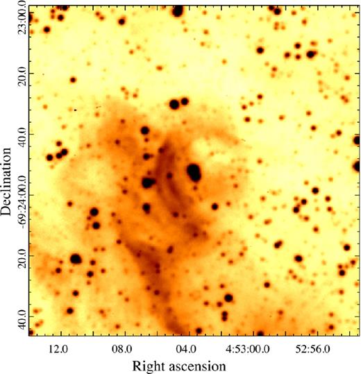
MCELS2 Hα image of the circular shell. BAT99 3a and star 2 are clearly resolved in the image. At the distance of the LMC of 50 kpc, 20 arcsec corresponds to ≈4.8 pc.
6.3 Spectroscopy of the shell
All long-slit spectra obtained with the Gemini and du Pont telescopes and the SALT show numerous emission lines along the whole slit. Intensities of these lines depend on weather conditions and the slit's PA. Some of the lines show spatial correlation with the shell. Below we analyse the obtained spectra to understand the origin of the shell.
6.3.1 Long-slit spectra of the shell
For the analysis of physical conditions and elemental abundances in the shell, all long-slit spectra were re-reduced in the same manner and corrected for the night-sky background and emission from the fore/background H ii region using spectral data outside the area of radius of 25 arcsec centred on BAT99 3a. The finally reduced SALT relative flux distribution for the WN star was used to construct the sensitivity curve for the du Pont data. Since the spectra were obtained under different weather conditions, only some of them show diagnostic lines with a good enough S/N ratio. For this reason, only the first Gemini, the second du Pont and both SALT spectra (see Table 2) were used in our following analysis.
One-dimensional (1D) spectra of the shell were extracted from the area of radius of 15 arcsec centred on BAT99 3a with the central ± 3 arcsec excluded to avoid the effect of BAT99 3a and star 2. The final 1D du Pont and SALT spectra with all identified emission lines are presented in Fig. 10. We do not show the Gemini spectrum because of its much worse quality caused by poor weather conditions during the observing run.
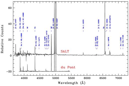
1D reduced spectra of the circular shell obtained with the SALT and du Pont telescopes (the du Pont spectrum is shifted downwards by 20 counts). All detected emission lines are marked.
All spectra show the nebular He ii λ4686 emission associated with the shell (see below). Only few such high-excitation nebulae are known in the Local Group (e.g. Garnett et al. 1991; Nazé et al. 2003; Pakull 2009; Kehrig et al. 2011) and most of them are associated with WNE, WC and WO stars, i.e. with WR stars capable of ionizing He ii.
Emission lines in the spectra of the shell were measured using programs described in detail in Kniazev et al. (2004, 2005). These programs determine the location of the continuum, perform a robust noise estimation and fit separate lines by a single Gaussian superimposed on the continuum-subtracted spectrum. Some overlapping lines were fitted simultaneously as a blend of two or more Gaussian features: the Hα λ6563 and [N ii] λλ6548, 6584 lines, the [S ii] λλ6716, 6731 lines, and the [O i] λ6300 and [S iii] λ6312 lines.
Table 7 lists the observed intensities of all detected lines normalized to Hβ, F(λ)/F(Hβ). To have independent estimates of the shell parameters, we combined the Gemini and du Pont data and analysed them separately from the SALT ones. The relative intensities of lines detected both in the Gemini and du Pont spectra, e.g. Hγ, [O iii] λ4363 and [O iii] λλ4959, 5007, are consistent with each other within the individual rms uncertainties (see columns 2 and 3 in Table 7) so that in the analysis based on the Gemini+du Pont data, we used the blue (<5876 Å) lines from the du Pont spectrum only and the red lines from the Gemini one. The combined SALT data cover the total spectral range 3700–7200 Å. The bluest (<4200 Å) and reddest (>6700 Å) lines in this data set have the largest relative errors because these lines were covered by only one observation (see Table 2). Since the Gemini+du Pont data set does not contain any of the O+ lines required to derive the O+/H+ abundance, we added to these data the intensity of the [O ii] λ3727 line from the combined SALT spectrum (see Table 7).
Line intensities of the shell.
| Gemini | du Pont | Gemini+du Pont | SALT | |||||
|---|---|---|---|---|---|---|---|---|
| λ0(Å) Ion | F(λ)/F(Hβ) | F(λ)/F(Hβ) | I(λ)/I(Hβ) | F(λ)/F(Hβ) | I(λ)/I(Hβ) | |||
| 3727 [O ii] | – | 0.755 ± 0.055a | 0.839 ± 0.064 | 0.755 ± 0.055 | 0.817 ± 0.061 | |||
| 3868 [Ne iii] | – | 0.420 ± 0.011 | 0.458 ± 0.012 | 0.396 ± 0.024 | 0.423 ± 0.026 | |||
| 3967 [Ne iii]+H7 | – | 0.222 ± 0.013 | 0.240 ± 0.015 | – | – | |||
| 4101 Hδ | – | 0.194 ± 0.006 | 0.207 ± 0.007 | 0.215 ± 0.029 | 0.226 ± 0.031 | |||
| 4340 Hγ | 0.508 ± 0.029 | 0.453 ± 0.011 | 0.472 ± 0.012 | 0.420 ± 0.017 | 0.434 ± 0.017 | |||
| 4363 [O iii] | 0.066 ± 0.017 | 0.069 ± 0.004 | 0.072 ± 0.005 | 0.059 ± 0.009 | 0.061 ± 0.009 | |||
| 4471 He i | – | 0.030 ± 0.002 | 0.031 ± 0.002 | 0.029 ± 0.011 | 0.029 ± 0.011 | |||
| 4686 He ii | 0.071 ± 0.014 | 0.071 ± 0.004 | 0.072 ± 0.004 | 0.062 ± 0.019 | 0.062 ± 0.020 | |||
| 4712 [Ar iv]+He i | – | 0.026 ± 0.003 | 0.026 ± 0.003 | – | – | |||
| 4861 Hβ | 1.000 ± 0.039 | 1.000 ± 0.030 | 1.000 ± 0.030 | 1.000 ± 0.043 | 1.000 ± 0.043 | |||
| 4959 [O iii] | 2.449 ± 0.076 | 2.423 ± 0.055 | 2.406 ± 0.055 | 2.317 ± 0.080 | 2.304 ± 0.079 | |||
| 5007 [O iii] | 7.221 ± 0.219 | 7.251 ± 0.163 | 7.172 ± 0.161 | 6.771 ± 0.213 | 6.713 ± 0.212 | |||
| 5876 He i | 0.114 ± 0.012 | – | 0.106 ± 0.011 | 0.133 ± 0.018 | 0.126 ± 0.018 | |||
| 6300 [O i] | – | – | – | 0.035 ± 0.005 | 0.033 ± 0.005 | |||
| 6312 [S iii] | – | – | – | 0.020 ± 0.005 | 0.019 ± 0.004 | |||
| 6548 [N ii] | 0.046 ± 0.010 | – | 0.042 ± 0.009 | 0.054 ± 0.004 | 0.049 ± 0.004 | |||
| 6563 Hα | 3.170 ± 0.092 | – | 2.859 ± 0.090 | 3.102 ± 0.097 | 2.852 ± 0.097 | |||
| 6584 [N ii] | 0.148 ± 0.013 | – | 0.134 ± 0.012 | 0.163 ± 0.009 | 0.149 ± 0.008 | |||
| 6678 He i | – | – | – | 0.060 ± 0.025 | 0.055 ± 0.023 | |||
| 6716 [S ii] | 0.264 ± 0.021 | – | 0.237 ± 0.019 | 0.194 ± 0.008 | 0.177 ± 0.007 | |||
| 6731 [S ii] | 0.200 ± 0.019 | – | 0.179 ± 0.017 | 0.142 ± 0.006 | 0.129 ± 0.006 | |||
| 7065 He i | – | – | – | 0.019 ± 0.012 | 0.017 ± 0.011 | |||
| 7136 [Ar iii] | – | – | – | 0.112 ± 0.017 | 0.100 ± 0.015 | |||
| C(Hβ) dex | 0.14 ± 0.04 | 0.11 ± 0.04 | ||||||
| E(B − V) mag | 0.10 ± 0.03 | 0.08 ± 0.04 | ||||||
aBased on the SALT data.
Table 7 also lists the reddening-corrected line intensity ratios, I(λ)/I(Hβ), and the logarithmic extinction coefficient, C(Hβ). The extinction coefficients derived from both sets of data (Gemini+du Pont and SALT) are consistent with each other and correspond to E(B − V) = 0.08–0.10 mag, which is a factor of 2 less than the colour excess derived for BAT99 3a and star 2 from the spectral analysis and photometry, respectively (see Sections 5 and 3.2.2). Since the spectra of the shell do not show any significant continuum (see Fig. 10), we assumed in our calculations that EW of underlying absorption in Balmer hydrogen lines is = 0 Å (cf. Kniazev et al. 2004, 2005).
6.3.2 Physical conditions and elemental abundances
To estimate the parameters of the shell, we used the technique of plasma diagnostics in the way described in full detail in Kniazev et al. (2008b). The electron temperature, Te([O iii]), was calculated using the weak auroral line of oxygen [O iii] λ4363, while the electron number density, ne([S ii]), was derived from the intensity ratio of the [S ii] λλ6716, 6731 lines.13 The estimates of ne based on the two data sets are consistent with each other and are typical of H ii regions and interstellar shells around WR stars (e.g. Esteban et al. 1992; Stock et al. 2011).
From the observed emission lines, we determined the abundances of O, N and Ne using the Gemini+du Pont data and those of O, N, Ne, S, Ar and He using the SALT data. As described in Kniazev et al. (2008b), we calculate ionic abundances, the ionization correction factors (ICFs) and total element abundances using system of equations from Izotov et al. (2006), which are based on sequences of photoionization models and used the new atomic data of Stasińska (2005). These abundances along with directly calculated Te, ne, ICFs for different elements, and total elemental abundances are listed in Table 8, where we also give the LMC abundances from Russell & Dopita (1992). Table 8 also shows Te([O ii]) and Te([S iii]), calculated using approximations from Izotov et al. (2006). We used Te([S iii]) for the calculation of S2 +/H+ and Ar2 +/H+ abundances. The detection of a strong nebular He ii λ4686 emission implies the presence of a non-negligible amount of O3 +, whose abundance can be derived in the way described in Izotov et al. (2006).
Elemental abundances in the shell.
| Quantity | Gemini+du Pont | SALT | LMCa |
|---|---|---|---|
| Te([O iii])(K) | 11,600 ± 300 | 11,200 ± 600 | – |
| Te([O ii])(K) | 12,000 ± 200 | 11,400 ± 200 | – |
| Te([S iii])(K) | – | 11,300 ± 760 | – |
| ne([S ii])(cm−3) | 90|$^{+200}_{-80}$| | 50|$^{+90}_{-40}$| | – |
| O+/H+(×105) | 1.615 ± 0.144 | 1.942 ± 0.189 | – |
| O++/H+(×105) | 16.200 ± 1.211 | 17.060 ± 2.812 | – |
| O++ +/H+(×105) | 1.349 ± 0.178 | 0.696 ± 0.377 | – |
| O/H( × 105) | 19.160 ± 1.779 | 19.700 ± 2.843 | – |
| 12+log(O/H) | 8.28 ± 0.03 | 8.29 ± 0.06 | 8.35 ± 0.06 |
| N+/H+(×107) | 15.870 ± 1.382 | 20.610 ± 1.253 | – |
| ICF(N) | 9.789 | 8.583 | – |
| N/H(×105) | 1.55 ± 0.14 | 1.77 ± 0.11 | – |
| 12+log(N/H) | 7.19 ± 0.04 | 7.25 ± 0.06 | 7.14 ± 0.15 |
| Ne++/H+(×105) | 2.841 ± 0.256 | 2.999 ± 0.608 | – |
| ICF(Ne) | 1.073 | 1.046 | – |
| Ne/H(×105) | 3.05 ± 0.28 | 3.14 ± 0.64 | – |
| 12+log(Ne/H) | 7.48 ± 0.05 | 7.50 ± 0.09 | 7.61 ± 0.05 |
| S+/H+(×107) | – | 5.119 ± 0.245 | – |
| S++/H+(×107) | – | 25.950 ± 9.201 | – |
| ICF(S) | – | 2.179 | – |
| S/H(×107) | – | 67.71 ± 20.06 | – |
| 12+log(S/H) | – | 6.83 ± 0.13 | 6.70 ± 0.09 |
| Ar++/H+(×107) | – | 6.952 ± 1.466 | – |
| ICF(Ar) | – | 1.240 | – |
| Ar/H(×107) | – | 8.62 ± 1.82 | – |
| 12+log(Ar/H) | – | 5.94 ± 0.09 | 6.29 ± 0.25 |
| 12+log(He/H) | – | 10.97 ± 0.05 | 10.94 ± 0.03 |
aThe LMC abundances are from Russell & Dopita (1992).
The helium abundance was derived in the manner described in detail in Izotov & Thuan (2004) and Izotov, Thuan & Lipovetsky (1994, 1997). The new fits from Benjamin, Skillman & Smith (2002) were used to convert He i emission line strengths to singly ionized helium abundances.
One can see that the shell abundances derived from both data sets are consistent with each other and the LMC ones within the error margins, which implies the absence of N and He enrichment of the shell and suggests that it is mainly composed of material swept-up from the local interstellar medium.
6.3.3 Position–velocity diagrams along the slit
To study the gas kinematics around BAT99 3a and star 2, we calculated the distribution of the heliocentric RV, Vhel, along the slit using both Gemini spectra and the method and programs described in Zasov et al. (2000). To exclude possible systematic shifts, the closest bright night sky line [O i] λ6363 Å was used. To match the scale along the slit with the seeing during the observations, the spectra were rebinned from 0.073 to 0.4 arcsec pixel−1. Finally, only those velocity measurements were used which satisfy the criteria S/N > 3 and σv < 5 km s−1.
The upper panels in Fig. 11 plot the Hα intensity and Vhel distributions along the slit for both Gemini spectra, obtained for PA = 125° (left-hand panel) and PA = 22°. In both cases, the Hα emission appears everywhere along the slit, but its intensity shows clear correlation with the shell (see the bottom-right panel for the MCELS2 Hα image of the shell with the slit positions for the Gemini observations shown by dashed lines). Particularly, it has two peaks in the south-east direction (at ≈8 and 13 arcsec from BAT99 3a), which correspond to the two arcs on the eastern side of the shell. In the north-west direction, the Hα emission peaks at ≈18 arcsec, which is consistent with the greater extent of the shell in this direction. One can also see that Vhel is quite uniform within the shell and in the south-east and south-west directions, and does not show a distinct correlation with the Hα intensity peaks. On the other hand, there is a noticeable increase of Vhel in the north-west direction, and to a lesser extent in the north-east one, suggesting that the shell might have a blister-like structure.
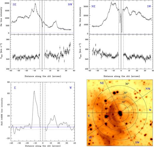
Upper panels: Hα line intensity and velocity profiles along the slit for two Gemini observations with PA = 125° (left-hand panel) and PA = 22°. SE–NW and NE–SW directions of the slit are shown. The solid vertical line corresponds to the position of BAT99 3a, while the dashed vertical lines (at ± 3 arcsec from the solid one) mark the area where the RV was not measured because of the effect of BAT99 3a and star 2. Bottom-left panel: He ii λ4686 line intensity profile along the slit for the second du Pont observation with PA = 90°. E–W direction of the slit is shown. The solid vertical line corresponds to the position of BAT99 3a. The solid horizontal line shows the background level and the dotted horizontal ones show ±1σ of the background noise. All data are background subtracted. Bottom-right panel: MCELS2 Hα image of the circular shell with the slit positions for the three above-mentioned observations indicated. Dashed lines correspond to the Gemini slits and the solid one to the du Pont slit. Concentric, dashed circles are overplotted on the image to make its comparison with the Hα and He ii λ4686 line intensities and Hα velocity profiles more convenient.
The bottom-left panel in Fig. 11 plots intensity of the He ii λ4686 line along the slit (indicated in the bottom-right panel by a solid line with PA = 90°) for the du Pont spectrum taken on 2012 December 13. One can see that the He ii emission shows a good correlation with the shell. Like the Hα emission, it is the brightest on the eastern edge of the shell and extends to a larger angular distance in the western direction. On the other hand, the He ii emission is concentrated only in the shell, which implies that the He iii region is trapped by the shell. It is instructive, therefore, to derive the effective temperature of the WR star by applying the Zanstra method (Zanstra 1927). With I(He ii λ4686)/I(Hβ) ≈ 0.07 (see Table 7) and using equation 1 in Kaler & Jacoby (1989), one finds Teff ≈ 95 kK, which agrees fairly well with the temperature derived in Section 5 (see Table 6).
6.4 Origin of the shell
In Section 6.3.2, we found that the chemical composition and electron number density of the shell are similar to those measured for H ii regions and interstellar shells around WR stars, which implies that the shell originated because of interaction between the WR wind and the local interstellar medium.14 This implication can be further supported by using diagnostic diagrams, which allow us to classify emission-line nebulae on the basis of line ratios (see e.g. Kniazev, Pustilnik & Zucker 2008a; Frew & Parker 2010, and references therein). With ratios log (I(Hα)/I([N ii] λλ6548,6584)) = 1.21, log (I(Hα)/I([S ii] λλ6717,6731)) = 0.84 and log (I([O iii] λ5007)/I(Hβ)) = 0.86, the shell is located in the region occupied by H ii regions and interstellar shells around Magellanic Cloud WR stars (see fig. 4 in Frew & Parker 2010). We therefore conclude that the circular shell is a wind-blown structure photoionized by its central stars.
We speculate that the two-arc morphology of the shell could be caused by a sharp density gradient along the line of sight, resulting in blow-up of the shell in the transverse direction as it entered in the region of lower density. This, along with the brightness asymmetry of the shell and the displacement of its central stars, provides support to the possibility that the shell is associated with a blister-like, wind-driven bubble.
7 DISCUSSION AND CONCLUSION
There is mounting evidence that massive stars form in a clustered way (Gvaramadze et al. 2012b and references therein). Subsequently, some of them found themselves in the field because of dynamical few-body encounters (Poveda et al. 1967; Gies & Bolton 1986), binary–supernova explosions (Blaauw 1961; Stone 1991) and cluster dissolution caused by gas expulsion (Tutukov 1978; Kroupa, Aarseth & Hurley 2001). The discovery of two massive and therefore rare stars, one of which in its turn is a massive binary system, at ≈0.5 pc in projection from each other, gives rise to the question of their physical relationship.
A chance projection along the same line of sight of physically unrelated massive field stars can be rejected to a considerable degree of reliability. Although such projections might be common in the vicinity of massive star clusters, they are highly improbable in the field (cf. Gvaramadze & Menten 2012). One can envisage two possible explanations of the close proximity of BAT99 3a and star 2.
First, these two stars might be members (at least in the recent past) of a runaway triple (or higher multiplicity) hierarchical system, which became unstable and dissolved into a binary system (now BAT99 3a) and a single unbound star (star 2) in the course of evolution of its most massive component(s) (e.g. Gvaramadze & Menten 2012). If this is the case, then the brightness asymmetry of the shell and the offset of the stars towards its brightest portion could be because of the eastward motion of the system. For a typical space velocity of runaway stars of several tens of km s−1 and assuming that the system was ejected ∼6 Myr ago (i.e. soon after its formation in the parent cluster), one finds that the cluster should be ∼100–200 pc away. Proceeding from this, we searched for known star clusters to the west of the shell and found two open clusters, [HS66] 49 and IC 2111, at ≈ 41 and 92 pc in projection, respectively (cf. Gvaramadze et al. 2012c). The age of the former cluster is unknown, while that of the latter one is 6 ± 1 Myr (Wolf et al. 2007), i.e. consistent with the age of the WN3 star of ≈6 Myr (see Section 5). The runaway scenario, however, implies that the circular shell should be of circumstellar origin (cf. Lozinskaya 1992; Danforth & Chu 2001; Gvaramadze et al. 2009), which is inconsistent with the normal chemical composition of the shell. It is likely therefore that the lopsided appearance of the shell and the displacement of its central stars are simply because of the eastward density gradient of the ambient medium (cf. Sections 2 and 6).
Secondly, BAT99 3a and star 2 could be members of a yet unrecognized star cluster. Observational and theoretical arguments suggest that star clusters are formed in compact configurations with the characteristic radius of ≤1 pc, which is independent of cluster mass (Kroupa & Boily 2002). This makes them hardly resolved in the Magellanic Clouds, where 1 pc corresponds to ≈3–4 arcsec. Indeed, some of the brightest stars in these galaxies are today known to be star clusters (e.g. Weigelt & Baier 1985; Walborn et al. 1995, 1999; Heydari-Malayeri et al. 2002). Moreover, the detection of young star clusters could additionally be hampered because of heavy obscuration by dust in their parent molecular clouds. Some members of these embedded clusters, however, could be visible in optical wavelengths if they were dynamically ejected out of the obscuring material (Gvaramadze et al. 2010a, 2012b) and/or if they are located in a favourably oriented blister-like H ii region on the near side of the natal cloud (cf. Gvaramadze et al. 2011b). It is possible that just this situation takes place in the case of BAT99 3a and star 2 (cf. Section 5), and that their cousins in the parent cluster are hidden by obscuring material along our line of sight.
To conclude, follow-up IR spectroscopy of star 3 is highly desirable to confirm its status as an O star and to prove the existence of a star cluster possibly associated with BAT99 3a and star 2. The latter in its turn would provide one more piece of evidence that massive stars form in a clustered mode.
ACKNOWLEDGEMENTS
Some observations reported in this paper were obtained with the Southern African Large Telescope (SALT). ANC gratefully acknowledges support from the Chilean Centro de Astrofísica FONDAP no. 15010003, the Chilean Centro de Excelencia en Astrofísica y Tecnologías Afines (CATA) BASAL PFB-06/2007, the Comite Mixto ESO-Gobierno de Chile and GEMINI-CONICYT no. 32110005. AYK acknowledges support from the National Research Foundation of South Africa. This work has made use of the NASA/IPAC Infrared Science Archive, which is operated by the Jet Propulsion Laboratory, California Institute of Technology, under contract with the National Aeronautics and Space Administration, the SIMBAD data base and the VizieR catalogue access tool, both operated at CDS, Strasbourg, France.
PACS=Photodetector Array Camera and Spectrometer (Poglitsch et al. 2010).
The resolution of these images is ≈12 and 6 arcsec, respectively.
SMC=Small Magellanic Cloud.
This survey, carried out with the Infrared Survey Facility 1.4-m telescope at Sutherland, the South African Astronomical Observatory, resolves neighbouring stars separated by more than ∼0.3 pc and its 10σ limiting magnitudes are 18.8, 17.8 and 16.6 mag at J, H and Ks, respectively, which are fainter by ≈2 mag than the two recent near-IR surveys, the 2MASS and the Deep Near Infrared Survey of the Southern Sky (DENIS Consortium 2005).
iraf: the Image Reduction and Analysis Facility is distributed by the National Optical Astronomy Observatory, which is operated by the Association of Universities for Research in Astronomy, Inc. under cooperative agreement with the National Science Foundation.
While the existence of an unresolved companion star generally affects the observed EWs, a subsequent spectral analysis (see Section 5) showed that the contribution of the WR star to the visual continuum is negligible, implying that the measured EWs of the classification absorption lines are very close to the intrinsic ones.
powr models of WR stars can be downloaded at http://www.astro.physik.uni-potsdam.de/PoWR.html.
See also http://bonnsai.astro.uni-bonn.de.
Although the [Ar iv] λλ4711, 4740 doublet is also present in the du Pont spectrum of the shell, we did not use it for density evaluation because of its weakness.
Note that the total mechanical luminosity of the O component of BAT99 3a and star 2 constitutes about 10 per cent of the mechanical luminosity of the WN3 star.
